Hopf bifurcation and periodic solutions in a coupled Brusselator model of chemical reactions

Yihuan Sun¹,  Shanshan Chen²¹¹1Corresponding Author, Email: [email protected]
¹ School of Mathematics, Harbin Institute of Technology,
  Harbin, Heilongjiang, 150001, P.R.China.
² Department of Mathematics, Harbin Institute of Technology,
  Weihai, Shandong, 264209, P.R.China.

Abstract

In this paper, we consider a coupled Brusselator model of chemical reactions, for which no symmetry for the coupling matrices is assumed. We show that the model can undergoes a Hopf bifurcation, and consequently periodic solutions can arise when the dispersal rates are large. Moreover, the effect of the coupling matrices on the Hopf bifurcation value is considered for a special case.

Keywords: Hopf bifurcation; Periodic solutions; Coupling matrix; Line-sum symmetric matrix.
MSC 2010: 34C23, 37G15, 92C40

1 Introduction

Nonlinear oscillations often occur in many chemical reactions and physical processes, [9, 17, 19]. For example, sustained oscillations in Brusselator model were studied in [19]. Brusselator model, proposed by Prigogine and Lefever [30], describes a set of chemical reactions as follows:

A\rightarrow X,\;\;B+X\rightarrow Y+C,\;\;2X+Y\rightarrow 3X,\;\;X\rightarrow D,

(1.1)

where $A$ and $B$ are the concentrations of the initial substances, $X$ and $Y$ are the concentrations of the intermediate reactants, and $C$ and $D$ are the concentrations of the final products. If the concentrations $A$ and $B$ depend only on space, these chemical reactions can be modelled by the following reaction-diffusion model: (see [19, 30])

\begin{cases}X_{t}=d_{1}\Delta X+A(x)-(B(x)+1)X+X^{2}Y,&x\in\Omega,\;t>0,\\ Y_{t}=d_{2}\Delta Y+B(x)X-X^{2}Y,&x\in\Omega,\;t>0.\end{cases}

(1.2)

Here $d_{1},d_{2}>0$ are the dispersal rates. If $A$ and $B$ are spatially homogeneous, then model (1.2) admits a unique constant steady state for the homogeneous Neumann boundary condition. One can refer to [7, 10, 21, 23, 25, 36, 39] and references therein for the results on steady state and Hopf bifurcations near this constant steady state. The global bifurcation theory and some other methods were used to show the existence of non-constant steady states for a wide range of parameters, see, e.g., [3, 14, 26, 27, 28]. Moreover, the effect of advection was considered in [2, 18], and the diffusion term in (1.2) was replaced by the following form:

d_{i}\displaystyle\frac{\partial^{2}}{\partial x^{2}}\to d_{i}\displaystyle\frac{\partial^{2}}{\partial x^{2}}-c_{i}\displaystyle\frac{\partial}{\partial x}

for the case that $\Omega$ is one dimension.

If chemical reactions (1.1) take places in $n$ -boxes, then model (1.2) takes the following discrete form:

\begin{cases}\displaystyle\frac{dx_{j}}{dt}=d_{1}\sum_{k=1}^{n}p_{jk}x_{k}+a_{j}-(\beta b_{j}+1)x_{j}+x_{j}^{2}y_{j},&j=1,\dots,n,\;\;t>0,\\ \displaystyle\frac{dy_{j}}{dt}=d_{2}\sum_{k=1}^{n}q_{jk}y_{k}+\beta b_{j}x_{j}-x_{j}^{2}y_{j},&j=1,\dots,n,\;\;t>0,\\ \bm{x}(0)=\bm{x}_{0}\geq(\not\equiv)\bm{0},\;\bm{y}(0)=\bm{y}_{0}\geq(\not\equiv)\bm{0}.\end{cases}

(1.3)

Here $n\geq 2$ is the number of boxes in chemical reactions; $\bm{x}=(x_{1},\dots,x_{n})^{T}$ and $\bm{y}=(y_{1},\dots,y_{n})^{T}$ , where $x_{j}$ and $y_{j}$ denote the concentrations of $X$ and $Y$ in box $i$ at time $t$ , respectively; the nonlinear term ${x_{j}^{2}}y_{j}$ describes the autocatalytic step in box $j$ ; and ${a_{j}}>0$ and $\beta{b_{j}}>0$ denote the input concentrations of initial substances $A$ and $B$ in box $j$ , respectively. We remark that $\beta$ introduced here is the scaling parameter, and we choose it as the bifurcation parameter. Moreover, $\left(p_{jk}\right)$ and $\left(q_{jk}\right)$ are the coupling matrices, where $p_{jk},q_{jk}(j\neq k)$ describe the rates of movement from box $k$ to box $j$ for the two reactants, respectively, and $p_{jj}(=-\sum_{k\neq j}p_{kj})$ and $q_{jj}(=-\sum_{k\neq j}q_{kj})$ denote the rates of leaving box $j$ for $j=1,\dots,n$ .

Model (1.3) was first considered by Prigogine and Lefever in [30] for the case of two boxes ( $n=2$ ), where the coupling matrices $\left(p_{jk}\right)$ and $\left(q_{jk}\right)$ were assumed to be symmetric, and the two boxes were identical (that is, $a_{1}=a_{2}=a$ and $b_{1}=b_{2}=1$ ). In this case, model (1.3) admits a unique space-independent steady state:

x_{i}=a,\;\;y_{i}=\beta/a\;\;\text{for}\;\;i=1,2,

and the existence of space-dependent steady state was showed in [30]. Model (1.3) with symmetric coupling matrices and identical boxes were also considered in [20, 22, 31, 32], where the steady state and Hopf bifurcation were studied in [20, 31]. One can also refer to [8, 29, 35, 40] and references therein for the steady state and Hopf bifurcations of other coupled models with symmetric coupling matrices.

It is well-known that the symmetric coupling matrices could mimic random diffusion, and the asymmetric case could mimic advective movements in the fluid. If the coupling matrices $\left(p_{jk}\right)$ and $\left(q_{jk}\right)$ are asymmetric, the steady states of model (1.3) are space-dependent even when the boxes are all identical. Consequently, we cannot obtain the explicit expression of the steady states, which brings difficulties in analyzing the Hopf bifurcation. In this paper, we aim to solve this problem and analyze the Hopf bifurcation of model (1.3).

Throughout the paper, we impose the following two assumptions:

$(\bf A_{1})$

The coupling matrices $P:=(p_{jk})$ and $Q:=(q_{jk})$ are irreducible and essentially nonnegative;
$(\bf A_{2})$

$\displaystyle\frac{d_{2}}{d_{1}}:=\theta>0$ .

Here we remark that real matrices with nonnegative off-diagonal elements are called essentially nonnegative. It follows from $(\bf A_{1})$ and Perron-Frobenius theorem that $s(P)=s(Q)=0$ , where $s(P)$ and $s(Q)$ are spectrum bounds of $P$ and $Q$ , respectively. Clearly, $s(P)$ and $s(Q)$ are also simple eigenvalues of $P$ and $Q$ with strongly positive eigenvectors ${\bm{\xi}}$ and ${\bm{\eta}}$ , respectively, where

\begin{split}&\bm{\xi}=(\xi_{1},\cdots,\xi_{n})^{T}\gg\bm{0},\;\;\text{and}\;\;\sum_{j=1}^{n}\xi_{j}=1,\\ &\bm{\eta}=(\eta_{1},\cdots,\eta_{n})^{T}\gg\bm{0},\;\;\text{and}\;\;\sum_{j=1}^{n}\eta_{j}=1.\\ \end{split}

(1.4)

Here $(x_{1},\cdots,x_{n})^{T}\gg\bm{0}$ represents that $x_{j}>0$ for $j=1,\dots,n$ . Assumption $(\bf A_{2})$ is a mathematically technical condition, and it means that the dispersal rates of the two reactants are proportional. Then letting $\tilde{t}=d_{1}t$ , denoting $\lambda=1/d_{1}$ , and dropping the tilde sign, model (1.3) can be transformed to the following equivalent model:

\begin{cases}\displaystyle\frac{dx_{j}}{dt}=\sum_{k=1}^{n}p_{jk}x_{k}+\lambda\left[a_{j}-(\beta b_{j}+1)x_{j}+x_{j}^{2}y_{j}\right],&j=1,\dots,n,\;\;t>0,\\ \displaystyle\frac{dy_{j}}{dt}=\theta\sum_{k=1}^{n}q_{jk}y_{k}+\lambda\left(\beta b_{j}x_{j}-x_{j}^{2}y_{j}\right),&j=1,\dots,n,\;\;t>0,\\ \bm{x}(0)=\bm{x}_{0}\geq(\not\equiv)\bm{0},\;\bm{y}(0)=\bm{y}_{0}\geq(\not\equiv)\bm{0},\end{cases}

(1.5)

where $\theta$ is defined in assumption $(\bf A_{2})$ .

We point out that the method in this paper is motivated by [4], where the steady state of the model is space-dependent. One can also refer to [1, 5, 6, 11, 12, 13, 15, 24, 34, 37, 38] on Hopf bifurcations near this type of steady state for delayed reaction-diffusion equations and delayed differential equations. We remark that, for the model in [4], the steady state does not depends on bifurcation parameter. But for patch models, the steady states always depend on the bifurcation parameter (see $\beta$ in model (1.5)), which brings some technical hurdles in analyzing Hopf bifurcations. Therefore, we need to improve the method in [4] here.

For simplicity, we use the following notations. We denote the complexification of a real linear space $\mathcal{Z}$ to be $\mathcal{Z}_{\mathbb{C}}:=\mathcal{Z}\oplus{\rm i}\mathcal{Z}=\{x_{1}+{\rm i}x_{2}|x_{1},x_{2}\in\mathcal{Z}\}$ , and define the kernel of a linear operator $T$ by $\mathcal{N}(T)$ . For $\mu\in\mathbb{C}$ , we define the real part by $\mathcal{R}e\mu$ . For the complex valued space $\mathbb{C}^{n}$ , we choose the standard inner product $\langle\bm{u},\bm{v}\rangle=\sum_{j=1}^{n}\overline{u}_{j}v_{j}$ , and consequently, the norm is defined by

\|\bm{u}\|_{2}=\left(\sum_{j=1}^{n}|u_{j}|^{2}\right)^{\frac{1}{2}}\;\;\text{for}\;\;\bm{u}\in\mathbb{C}^{n}.

Moreover, for $\bm{x}=(x_{1},\dots,x_{n})^{T},\bm{y}=(y_{1},\dots,y_{n})^{T}\in\mathbb{C}^{n}$ , we denote

(\bm{x},\bm{y})^{T}=\left({\begin{array}[]{c}{\bm{x}}\\ {\bm{y}}\end{array}}\right)=(x_{1},\dots,x_{n},y_{1},\dots,y_{n})^{T}.

The rest of the paper is organized as follows. In Section 2, we study the existence and uniqueness of the positive equilibrium for model (1.5) (or respectively, (1.3)). In Section 3, we show the existence of Hopf bifurcation and the stability of the positive equilibrium for model (1.5) (or respectively, (1.3)) when $\lambda$ is small. In Section 4, we show the effect of the coupling matrices on the Hopf bifurcation value for a special case. Finally, some numerical simulations are provided to illustrate the theoretical results.

2 Existence of positive equilibria

In this section, we consider the existence of positive equilibria of model (1.5), which satisfy

\begin{cases}\sum_{k=1}^{n}p_{jk}x_{k}+\lambda\left[a_{j}-(\beta b_{j}+1)x_{j}+x_{j}^{2}y_{j}\right]=0,&j=1,\dots,n,\\ \theta\sum_{k=1}^{n}q_{jk}y_{k}+\lambda\left(\beta b_{j}x_{j}-x_{j}^{2}y_{j}\right)=0,&j=1,\dots,n.\end{cases}

(2.1)

Note that $(\bm{x},\bm{y})=(c\bm{\xi},d\bm{\eta})$ solves (2.1) for all $c,d\in\mathbb{R}$ when $\lambda=0$ . Therefore, we cannot solve (2.1) by the direct application of the implicit function theorem. We need to split the phase space and find an equivalent system of (2.1). It is well-known that

\mathbb{R}^{n}={\rm span}\{\bm{\xi}\}\oplus\mathcal{M}={\rm span}\{\bm{\eta}\}\oplus\mathcal{M},

where $\bm{\xi}$ and $\bm{\eta}$ are defined in (1.4), and

\mathcal{M}:=\left\{\bm{x}=(x_{1},\dots,x_{n})^{T}\in\mathbb{R}^{n}:\sum_{j=1}^{n}x_{j}=0\right\}.

Letting

\begin{split}&\bm{x}=c\bm{\xi}+\bm{u},\;\;c\in\mathbb{R},\;\bm{u}\in\mathcal{M},\\ &\bm{y}=r\bm{\eta}+\bm{v},\;\;r\in\mathbb{R},\;\bm{v}\in\mathcal{M},\\ \end{split}

(2.2)

and plugging (2.2) into (2.1), we see that $(\bm{x},\bm{y})$ (defined in (2.2)) is a solution of (2.1), if and only if $(c,r,\bm{u},\bm{v})\in\mathbb{R}^{2}\times\mathcal{M}^{2}$ solves

\bm{F}(c,r,\bm{u},\bm{v},\beta,\lambda)=(f_{1},f_{21},\dots,f_{2n},f_{3},f_{41},\dots,f_{4n})^{T}=\bm{0},

(2.3)

where $\bm{F}(c,r,\bm{u},\bm{v},\beta,\lambda):\mathbb{R}^{2}\times\mathcal{M}^{2}\times\mathbb{R}^{2}\to\left(\mathbb{R}\times\mathcal{M}\right)^{2}$ , and

\begin{cases}f_{1}(c,r,\bm{u},\bm{v},\beta,\lambda):=\displaystyle\sum_{j=1}^{n}\left[a_{j}-(\beta b_{j}+1)(c\xi_{j}+u_{j})+(c\xi_{j}+u_{j})^{2}(r\eta_{j}+v_{j})\right],\\ f_{2j}(c,r,\bm{u},\bm{v},\beta,\lambda):=\lambda\left[a_{j}-(\beta b_{j}+1)(c\xi_{j}+u_{j})+(c\xi_{j}+u_{j})^{2}(r\eta_{j}+v_{j})\right]\\ ~{}~{}~{}~{}~{}~{}~{}~{}~{}~{}~{}~{}~{}~{}~{}~{}~{}~{}~{}~{}~{}~{}~{}~{}~{}~{}~{}\displaystyle+\sum_{k=1}^{n}p_{jk}u_{k}-\displaystyle\frac{\lambda}{n}f_{1},~{}~{}~{}~{}~{}~{}j=1,\dots,n,\\ f_{3}(c,r,\bm{u},\bm{v},\beta,\lambda):=\displaystyle\sum_{j=1}^{n}\left[\beta b_{j}(c\xi_{j}+u_{j})-(c\xi_{j}+u_{j})^{2}(r\eta_{j}+v_{j})\right],\\ f_{4j}(c,r,\bm{u},\bm{v},\beta,\lambda):=\lambda\left[\beta b_{j}(c\xi_{j}+u_{j})-(c\xi_{j}+u_{j})^{2}(r\eta_{j}+v_{j})\right]\\ ~{}~{}~{}~{}~{}~{}~{}~{}~{}~{}~{}~{}~{}~{}~{}~{}~{}~{}~{}~{}~{}~{}~{}~{}~{}~{}~{}\displaystyle+\theta\sum_{k=1}^{n}q_{jk}v_{k}-\displaystyle\frac{\lambda}{n}f_{3},~{}~{}~{}~{}~{}~{}j=1,\dots,n.\\ \end{cases}

(2.4)

We first solve $\bm{F}(c,r,\bm{u},\bm{v},\beta,\lambda)=\bm{0}$ for $\lambda=0$ .

Lemma 2.1.

Assume that $\lambda=0$ . For fixed $\beta>0$ , $\bm{F}(c,r,\bm{u},\bm{v},\beta,\lambda)=\bm{0}$ has a unique solution $(c_{0},r_{0\beta},\bm{u}_{0},\bm{v}_{0})\in\mathbb{R}^{2}\times\mathcal{M}^{2}$ , where

c_{0}=\sum_{j=1}^{n}a_{j},\;\;r_{0\beta}=\frac{\beta\sum_{j=1}^{n}b_{j}\xi_{j}}{\left(\sum_{j=1}^{n}a_{j}\right)\left(\sum_{j=1}^{n}\xi_{j}^{2}\eta_{j}\right)},\;\;\bm{u}_{0}=\bm{0},\;\;\bm{v}_{0}=\bm{0}.

(2.5)

Proof.

Plugging $\lambda=0$ into $f_{2j}=f_{4j}=0$ for $j=1,\dots,n$ , we have $\bm{u}=\bm{u}_{0}=\bm{0}$ and $\bm{v}=\bm{v}_{0}=\bm{0}$ . Then plugging $\bm{u}=\bm{v}=\bm{0}$ into $f_{1}=f_{3}=0$ , we have

\sum_{j=1}^{n}\left[a_{j}-c(\beta b_{j}+1)\xi_{j}+c^{2}r\xi_{j}^{2}\eta_{j}\right]=0,\;\;\sum_{j=1}^{n}\left[c\beta b_{j}\xi_{j}-c^{2}r\xi_{j}^{2}\eta_{j}\right]=0,

which implies that

c=c_{0}=\sum_{j=1}^{n}a_{j},\;\;r=r_{0\beta}=\frac{\beta\sum_{j=1}^{n}b_{j}\xi_{j}}{\left(\sum_{j=1}^{n}a_{j}\right)\left(\sum_{j=1}^{n}\xi_{j}^{2}\eta_{j}\right)}.

This completes the proof. ∎

Now we solve (2.1) (or equivalently, (2.3)) for $\lambda>0$ .

Theorem 2.2.

For any fixed $\beta_{1}>0$ , there exists $\delta_{\beta_{1}}\in(0,\beta_{1})$ and a continuously differentiable mapping $\left(\bm{x}^{(\lambda,\beta)},\bm{y}^{(\lambda,\beta)}\right):[0,\delta_{\beta_{1}}]\times[\beta_{1}-\delta_{\beta_{1}},\beta_{1}+\delta_{\beta_{1}}]\to\mathbb{R}^{n}\times\mathbb{R}^{n}$ such that $(\bm{x}^{(\lambda,\beta)},\bm{y}^{(\lambda,\beta)})$ is the unique positive solution of (2.1) for $(\lambda,\beta)\in(0,\delta_{\beta_{1}}]\times[\beta_{1}-\delta_{\beta_{1}},\beta_{1}+\delta_{\beta_{1}}]$ . Moreover,

\bm{x}^{(\lambda,\beta)}=c^{(\lambda,\beta)}\bm{\xi}+\bm{u}^{(\lambda,\beta)},\;\;\bm{y}^{(\lambda,\beta)}=r^{(\lambda,\beta)}\bm{\eta}+\bm{v}^{(\lambda,\beta)},

(2.6)

where $\left(c^{(\lambda,\beta)},r^{(\lambda,\beta)},\bm{u}^{(\lambda,\beta)},\bm{v}^{(\lambda,\beta)}\right)\in\mathbb{R}^{2}\times\mathcal{M}^{2}$ solves Eq. (2.3) for $(\lambda,\beta)\in[0,\delta_{\beta_{1}}]\times[\beta_{1}-\delta_{\beta_{1}},\beta_{1}+\delta_{\beta_{1}}]$ , and

\left(c^{(0,\beta)},r^{(0,\beta)},\bm{u}^{(0,\beta)},\bm{v}^{(0,\beta)}\right)=(c_{0},r_{0\beta},\bm{0},\bm{0})\;\;\text{for}\;\;\beta\in[\beta_{1}-\delta_{\beta_{1}},\beta_{1}+\delta_{\beta_{1}}],

(2.7)

with $c_{0}$ and $r_{0\beta}$ defined in Lemma 2.1.

Proof.

We first show the existence. It follows from Lemma 2.1 that

\bm{F}(c_{0},r_{0\beta_{1}},\bm{0},\bm{0},\beta_{1},0)=\bm{0},

where $\bm{F}$ is defined in (2.3). A direct computation implies that the Fréchet derivative of $\bm{F}$ with respect to $(c,r,\bm{u},\bm{v})$ at $(c_{0},r_{0\beta_{1}},\bm{0},\bm{0},\beta_{1},0)$ is as follows:

\bm{G}(\tilde{c},\tilde{r},\bm{\tilde{u}},\bm{\tilde{v}})=(g_{1},g_{21},\dots,g_{2n},g_{3},g_{41},\dots,g_{4n})^{T},

where $\tilde{c},\tilde{r}\in\mathbb{R}$ , $\bm{\tilde{u}},\bm{\tilde{v}}\in\mathcal{M}$ , and

\begin{cases}\displaystyle g_{1}(\tilde{c},\tilde{r},\bm{\tilde{u}},\bm{\tilde{v}}):=\sum_{j=1}^{n}\left[{\left(2c_{0}r_{0\beta_{1}}\xi_{j}\eta_{j}-\beta_{1}b_{j}-1\right){(\tilde{c}\xi_{j}+\tilde{u}_{j})}+{(c_{0}\xi_{j})}^{2}}{(\tilde{r}\eta_{j}+\tilde{v}_{j})}\right],\\ \displaystyle g_{2j}(\tilde{c},\tilde{r},\bm{\tilde{u}},\bm{\tilde{v}}):=\sum_{k=1}^{n}{p_{jk}\tilde{u}_{k}},~{}~{}~{}~{}~{}~{}j=1,\dots,n,\\ \displaystyle g_{3}(\tilde{c},\tilde{r},\bm{\tilde{u}},\bm{\tilde{v}}):=\sum_{j=1}^{n}\left[{\left(\beta_{1}b_{j}-2c_{0}r_{0\beta_{1}}\xi_{j}\eta_{j}\right){(\tilde{c}\xi_{j}+\tilde{u}_{j})}-{(c_{0}\xi_{j})}^{2}}{(\tilde{r}\eta_{j}+\tilde{v}_{j})}\right],\\ \displaystyle g_{4j}(\tilde{c},\tilde{r},\bm{\tilde{u}},\bm{\tilde{v}}):=\theta\sum_{k=1}^{n}{q_{jk}\tilde{v}_{k}},~{}~{}~{}~{}~{}~{}j=1,\dots,n.\\ \end{cases}

If $\bm{G}(\tilde{c},\tilde{r},\bm{\tilde{u}},\bm{\tilde{v}})=\bm{0}$ , then $\bm{\tilde{u}}=\bm{0}$ and $\bm{\tilde{v}}=\bm{0}$ . Plugging $\bm{\tilde{u}}=\bm{\tilde{v}}=\bm{0}$ into $g_{1}=g_{3}=0$ , we have

\left(\begin{array}[]{cc}\sum_{j=1}^{n}\left(2c_{0}r_{0\beta_{1}}\xi_{j}\eta_{j}-\beta_{1}b_{j}-1\right)\xi_{j}&\sum_{j=1}^{n}{(c_{0}\xi_{j})}^{2}\eta_{j}\\ \sum_{j=1}^{n}\left(\beta_{1}b_{j}-2c_{0}r_{0\beta_{1}}\xi_{j}\eta_{j}\right)\xi_{j}&-\sum_{j=1}^{n}{(c_{0}\xi_{j})}^{2}\eta_{j}\end{array}\right)\left({\begin{array}[]{*{20}{c}}\tilde{c}\\ \tilde{r}\end{array}}\right)=\left({\begin{array}[]{*{20}{c}}0\\ 0\end{array}}\right).

Noticing that

\left|\begin{array}[]{cc}\sum_{j=1}^{n}\left(2c_{0}r_{0\beta_{1}}\xi_{j}\eta_{j}-\beta_{1}b_{j}-1\right)\xi_{j}&\sum_{j=1}^{n}{(c_{0}\xi_{j})}^{2}\eta_{j}\\ \sum_{j=1}^{n}\left(\beta_{1}b_{j}-2c_{0}r_{0\beta_{1}}\xi_{j}\eta_{j}\right)\xi_{j}&-\sum_{j=1}^{n}{(c_{0}\xi_{j})}^{2}\eta_{j}\end{array}\right|\neq 0,

we obtain that $\tilde{c}=0$ and $\tilde{r}=0$ . Therefore, $\bm{G}$ is bijective.

It follows from the implicit function theorem that there exist $\delta_{\beta_{1}}\in(0,\beta_{1})$ and a continuously differentiable mapping

(\lambda,\beta)\in[0,\delta_{\beta_{1}}]\times[\beta_{1}-\delta_{\beta_{1}},\beta_{1}+\delta_{\beta_{1}}]\mapsto\left(c^{(\lambda,\beta)},r^{(\lambda,\beta)},\bm{u}^{(\lambda,\beta)},\bm{v}^{(\lambda,\beta)}\right)\in\mathbb{R}^{2}\times\mathcal{M}^{2}

such that $\bm{F}\left(c^{(\lambda,\beta)},r^{(\lambda,\beta)},\bm{u}^{(\lambda,\beta)},\bm{v}^{(\lambda,\beta)},\beta,\lambda\right)=\bm{0}$ and

\left(c^{(0,\beta_{1})},r^{(0,\beta_{1})},\bm{u}^{(0,\beta_{1})},\bm{v}^{(0,\beta_{1})}\right)=(c_{0},r_{0\beta_{1}},\bm{0},\bm{0}).

Then we can choose $\delta_{\beta_{1}}>0$ (sufficiently small) such that $\left(\bm{x}^{(\lambda,\beta)},\bm{y}^{(\lambda,\beta)}\right)$ (defined in (2.6)) is a positive solution of (2.1) for $(\lambda,\beta)\in(0,\delta_{\beta_{1}}]\times[\beta_{1}-\delta_{\beta_{1}},\beta_{1}+\delta_{\beta_{1}}]$ .

Now, we show the uniqueness. From the implicit function theorem, we only need to verify that if $\left(\bm{\tilde{x}}^{(\lambda,\beta)},\bm{\tilde{y}}^{(\lambda,\beta)}\right)$ is a positive solution of (2.1), where

\bm{\tilde{x}}^{(\lambda,\beta)}=\tilde{c}^{(\lambda,\beta)}\bm{\xi}+\bm{\tilde{u}}^{(\lambda,\beta)},\;\bm{\tilde{y}}^{(\lambda,\beta)}=\tilde{r}^{(\lambda,\beta)}\bm{\eta}+\bm{\tilde{v}}^{(\lambda,\beta)},\;\tilde{c}^{(\lambda,\beta)},\tilde{r}^{(\lambda,\beta)}\in\mathbb{R},\;\bm{\tilde{u}}^{(\lambda,\beta)},\bm{\tilde{v}}^{(\lambda,\beta)}\in\mathcal{M},

then $\left(\tilde{c}^{(\lambda,\beta)},\tilde{r}^{(\lambda,\beta)},\bm{\tilde{u}}^{(\lambda,\beta)},\bm{\tilde{v}}^{(\lambda,\beta)}\right)\to(c_{0},r_{0\beta_{1}},\bm{0},\bm{0})$ as $(\lambda,\beta)\to(0,\beta_{1})$ . Substituting $(c,r,\bm{u},\bm{v})=\left(\tilde{c}^{(\lambda,\beta)},\tilde{r}^{(\lambda,\beta)},\bm{\tilde{u}}^{(\lambda,\beta)},\bm{\tilde{v}}^{(\lambda,\beta)}\right)$ into (2.3), we see from the first and third equation of (2.4) that

\tilde{c}^{(\lambda,\beta)}=\sum_{j=1}^{n}{\tilde{x}_{j}^{(\lambda,\beta)}}=\sum_{j=1}^{n}a_{j},

which implies that $\bm{\tilde{u}}^{(\lambda,\beta)}$ is bounded in $\mathbb{R}^{n}$ . Then, up to a subsequence, we assume that

\lim_{(\lambda,\beta)\to(0,\beta_{1})}\bm{\tilde{u}}^{(\lambda,\beta)}=\bm{u}^{*}\in\mathcal{M}.

From the third equation of (2.4), we have

\sum_{j=1}^{n}\beta b_{j}\tilde{x}_{j}^{(\lambda,\beta)}=\sum_{j=1}^{n}\left(\tilde{x}_{j}^{(\lambda,\beta)}\right)^{2}\tilde{y}_{j}^{(\lambda,\beta)},

(2.8)

which implies that $\left\{\left(\tilde{x}_{j}^{(\lambda,\beta)}\right)^{2}\tilde{y}_{j}^{(\lambda,\beta)}\right\}_{j=1}^{n}$ are bounded. Taking the limit of

f_{2j}\left(\tilde{c}^{(\lambda,\beta)},\tilde{r}^{(\lambda,\beta)},\bm{\tilde{u}}^{(\lambda,\beta)},\bm{\tilde{v}}^{(\lambda,\beta)},\beta,\lambda\right)=0\;\;\text{for}\;\;j=1,\dots,n,

as $(\lambda,\beta)\to(0,\beta_{1})$ , we see that $P\bm{u}^{*}=\bm{0}$ , which yields $\bm{u}^{*}=\bm{0}$ . Therefore,

\lim_{(\lambda,\beta)\to(0,\beta_{1})}\bm{\tilde{u}}^{(\lambda,\beta)}=\bm{0}\;\;\;\;\text{and}\;\;\lim_{(\lambda,\beta)\to(0,\beta_{1})}\tilde{c}^{(\lambda,\beta)}=c_{0}.

(2.9)

It follows from (2.8) and (2.9) that $\bm{\tilde{y}}^{(\lambda,\beta)}$ is also bounded in $\mathbb{R}^{n}$ . Then, up to a subsequence, we assume that

\lim_{(\lambda,\beta)\to(0,\beta_{1})}\tilde{r}^{(\lambda,\beta)}=r^{*}\geq 0\;\;\;\;\text{and}\;\lim_{(\lambda,\beta)\to(0,\beta_{1})}\bm{\tilde{v}}^{(\lambda,\beta)}=\bm{v}^{*}\in\mathcal{M}.

Taking the limit of

f_{4j}\left(\tilde{c}^{(\lambda,\beta)},\tilde{r}^{(\lambda,\beta)},\bm{\tilde{u}}^{(\lambda,\beta)},\bm{\tilde{v}}^{(\lambda,\beta)},\beta,\lambda\right)=0\;\;\text{for}\;\;j=1,\dots,n,

as $(\lambda,\beta)\to(0,\beta_{1})$ , we see that $Q\bm{v}^{*}=\bm{0}$ , which yields $\bm{v}^{*}=\bm{0}$ . Consequently, taking the limit of

f_{3}\left(\tilde{c}^{(\lambda,\beta)},\tilde{r}^{(\lambda,\beta)},\bm{\tilde{u}}^{(\lambda,\beta)},\bm{\tilde{v}}^{(\lambda,\beta)},\beta,\lambda\right)=0

as $(\lambda,\beta)\to(0,\beta_{1})$ , we have $r^{*}=r_{0\beta_{1}}$ . Therefore,

\lim_{(\lambda,\beta)\to(0,\beta_{1})}\bm{\tilde{v}}^{(\lambda,\beta)}=\bm{0}\;\;\;\;\text{and}\;\;\lim_{(\lambda,\beta)\to(0,\beta_{1})}\tilde{r}^{(\lambda,\beta)}=r_{0\beta_{1}}.

Finally, we need to show that (2.7) holds. We can use the similar arguments as in the proof of the uniqueness, and here we omit the proof. ∎

In the above Theorem 2.2, we solve (2.1) when $\beta$ is in a small neighborhood of a given positive constant $\beta_{1}$ . In the following, we will consider the solution of (2.1) for a wider range of $\beta$ .

Theorem 2.3.

Let $\mathcal{B}:=[\epsilon,1/\epsilon]$ , where $\epsilon>0$ is sufficiently small. Then there exists $\delta_{\epsilon}>0$ and a continuously differentiable mapping $\left(\bm{x}^{(\lambda,\beta)},\bm{y}^{(\lambda,\beta)}\right):[0,\delta_{\epsilon}]\times\mathcal{B}\to\mathbb{R}^{n}\times\mathbb{R}^{n}$ such that $(\bm{x}^{(\lambda,\beta)},\bm{y}^{(\lambda,\beta)})$ is the unique positive solution of (2.1) for $(\lambda,\beta)\in(0,\delta_{\epsilon}]\times\mathcal{B}$ . Moreover,

\bm{x}^{(\lambda,\beta)}=c^{(\lambda,\beta)}\bm{\xi}+\bm{u}^{(\lambda,\beta)},\;\;\bm{y}^{(\lambda,\beta)}=r^{(\lambda,\beta)}\bm{\eta}+\bm{v}^{(\lambda,\beta)},

(2.10)

\left(c^{(0,\beta)},r^{(0,\beta)},\bm{u}^{(0,\beta)},\bm{v}^{(0,\beta)}\right)=(c_{0},r_{0\beta},\bm{0},\bm{0})\;\;\text{for}\;\;\beta\in\mathcal{B},

(2.11)

with $c_{0}$ and $r_{0\beta}$ defined in Lemma 2.1.

Proof.

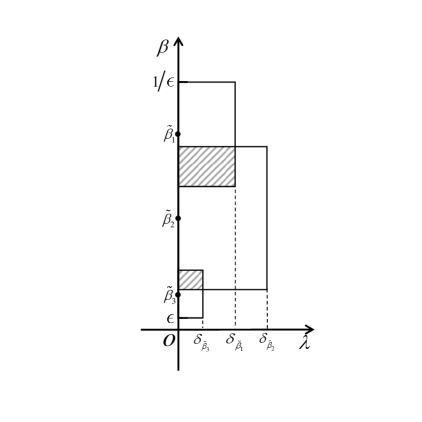
It follows from Theorem 2.2, for any $\tilde{\beta}\in\mathcal{B}$ , there exists $\delta_{\tilde{\beta}}\in(0,\tilde{\beta})$ such that, for $(\lambda,\beta)\in(0,\delta_{\tilde{\beta}}]\times[\tilde{\beta}-\delta_{\tilde{\beta}},\tilde{\beta}+\delta_{\tilde{\beta}}]$ , (2.1) admits a unique positive solution $(\bm{x}^{(\lambda,\beta)},\bm{y}^{(\lambda,\beta)})$ , where $\bm{x}^{(\lambda,\beta)}$ and $\bm{y}^{(\lambda,\beta)}$ are defined in (2.6) and continuously differentiable for $(\lambda,\beta)\in[0,\delta_{\tilde{\beta}}]\times[\tilde{\beta}-\delta_{\tilde{\beta}},\tilde{\beta}+\delta_{\tilde{\beta}}]$ . Clearly,

\mathcal{B}\subseteq\bigcup_{\tilde{\beta}\in\mathcal{B}}{\left({\tilde{\beta}-\delta_{\tilde{\beta}},\tilde{\beta}+\delta_{\tilde{\beta}}}\right)}.

Noticing that $\mathcal{B}$ is compact, we see that there exist finite open intervals (see Fig. 1), denoted by $\left({\tilde{\beta}_{l}}-\delta_{\tilde{\beta}_{l}},{\tilde{\beta}_{l}}+\delta_{\tilde{\beta}_{l}}\right)$ for $l=1,\dots,s$ , such that

\mathcal{B}\subseteq\bigcup_{l=1}^{s}{\left({\tilde{\beta}_{l}}-\delta_{\tilde{\beta}_{l}},{\tilde{\beta}_{l}}+\delta_{\tilde{\beta}_{l}}\right)}.

Choose $\delta_{\epsilon}=\min_{1\leq l\leq s}\delta_{\tilde{\beta}_{l}}$ . Then, for $(\lambda,\beta)\in(0,\delta_{\epsilon}]\times\mathcal{B}$ , (2.1) admits a unique positive solution $(\bm{x}^{(\lambda,\beta)},\bm{y}^{(\lambda,\beta)})$ , which is defined in (2.10) and continuously differentiable for $(\lambda,\beta)\in[0,\delta_{\epsilon}]\times\mathcal{B}$ . Eq. (2.11) can be proved by using the similar arguments as in the proof of Theorem 2.2, and here we omit the proof. ∎

Refer to caption — Figure 1: Finite open intervals covering $\mathcal{B}$ .

3 Stability and Hopf bifurcation

Throughout this section, we assume that $\beta\in\mathcal{B}$ , where $\mathcal{B}$ is defined in Theorem 2.3. It follows from Theorem 2.3 that there exists $\delta_{\epsilon}>0$ such that, for $(\lambda,\beta)\in(0,\delta_{\epsilon}]\times\mathcal{B}$ , (1.5) admits a unique positive equilibrium $(\bm{x}^{(\lambda,\beta)},\bm{y}^{(\lambda,\beta)})$ , where $\bm{x}^{(\lambda,\beta)}$ and $\bm{y}^{(\lambda,\beta)}$ are defined in (2.10). Here we use $\beta$ as the bifurcation parameter, and we will show that there exists a Hopf bifurcation curve $\beta=\beta_{\lambda}$ when $\lambda$ is small, see Fig. 2.

Linearizing model (1.5) at $(\bm{x}^{(\lambda,\beta)},\bm{y}^{(\lambda,\beta)})$ , we obtain

\begin{cases}\displaystyle\frac{d\tilde{x}_{j}}{dt}=\sum_{k=1}^{n}p_{jk}\tilde{x}_{k}+\lambda\left[M_{1j}^{(\lambda,\beta)}\tilde{x}_{j}+M_{2j}^{(\lambda,\beta)}\tilde{y}_{j}\right],~{}~{}~{}~{}j=1,\dots,n,\;t>0,\\ \displaystyle\frac{d\tilde{y}_{j}}{dt}=\theta\sum_{k=1}^{n}q_{jk}\tilde{y}_{k}+\lambda\left[M_{3j}^{(\lambda,\beta)}\tilde{x}_{j}-M_{2j}^{(\lambda,\beta)}\tilde{y}_{j}\right],~{}~{}~{}~{}j=1,\dots,n,\;t>0,\\ \end{cases}

where

M_{1j}^{(\lambda,\beta)}=2x_{j}^{(\lambda,\beta)}y_{j}^{(\lambda,\beta)}-\beta b_{j}-1,\;\;M_{2j}^{(\lambda,\beta)}={\left(x_{j}^{(\lambda,\beta)}\right)}^{2},\;\;M_{3j}^{(\lambda,\beta)}=\beta b_{j}-2x_{j}^{(\lambda,\beta)}y_{j}^{(\lambda,\beta)}.

(3.1)

Let

A_{\beta}(\lambda):=\left({\begin{array}[]{*{20}{c}}P&0\\ 0&\theta Q\end{array}}\right)+\lambda\left({\begin{array}[]{*{20}{c}}M_{1}&M_{2}\\ M_{3}&-M_{2}\end{array}}\right),

(3.2)

where $M_{1}={\rm diag}\left(M_{1j}^{(\lambda,\beta)}\right),M_{2}={\rm diag}\left(M_{2j}^{(\lambda,\beta)}\right)$ and $M_{3}={\rm diag}\left(M_{3j}^{(\lambda,\beta)}\right)$ . Then, $\mu\in\mathbb{C}$ is an eigenvalue of $A_{\beta}(\lambda)$ if there exists $(\bm{\varphi},\bm{\psi})^{T}(\neq\bm{0})\in\mathbb{C}^{2n}$ such that

\begin{cases}\displaystyle\mu\varphi_{j}=\sum_{k=1}^{n}p_{jk}\varphi_{k}+\lambda\left[M_{1j}^{(\lambda,\beta)}\varphi_{j}+M_{2j}^{(\lambda,\beta)}\psi_{j}\right],&j=1,\dots,n,\\ \displaystyle\mu\psi_{j}=\theta\sum_{k=1}^{n}q_{jk}\psi_{k}+\lambda\left[M_{3j}^{(\lambda,\beta)}\varphi_{j}-M_{2j}^{(\lambda,\beta)}\psi_{j}\right],&j=1,\dots,n.\\ \end{cases}

(3.3)

For further application, we first give a priori estimates for solutions of eigenvalue problem (3.3).

Lemma 3.1.

Let $\mathcal{B}$ and $\delta_{\epsilon}$ are defined in Theorem 2.3. Assume that, for $\lambda\in(0,\delta_{\epsilon}]$ , $(\mu_{\lambda},\beta_{\lambda},\bm{\varphi}_{\lambda},\bm{\psi}_{\lambda})$ solves (3.3) with $\mathcal{R}e\mu_{\lambda}\geq 0$ , $(\bm{\varphi}_{\lambda},\bm{\psi}_{\lambda})^{T}(\neq\bm{0})\in\mathbb{C}^{2n}$ and $\beta_{\lambda}\in\mathcal{B}$ . Then there exists $\lambda_{1}\in(0,\delta_{\epsilon})$ such that $\left|\mu_{\lambda}/\lambda\right|$ is bounded for $\lambda\in(0,{\lambda}_{1}]$ .

Proof.

Ignoring a scalar factor, we assume that $\|\bm{\varphi}_{\lambda}\|_{2}^{2}+\|\bm{\psi}_{\lambda}\|_{2}^{2}=\|\bm{\xi}\|_{2}^{2}+\|\bm{\eta}\|_{2}^{2}$ , where $\bm{\xi}$ and $\bm{\eta}$ are defined in (1.4). Substituting $(\mu,\beta,\bm{\varphi},\bm{\psi})=(\mu_{\lambda},\beta_{\lambda},\bm{\varphi}_{\lambda},\bm{\psi}_{\lambda})$ into (3.3), we have

\begin{cases}\displaystyle\mu_{\lambda}\varphi_{\lambda j}=\sum_{k=1}^{n}p_{jk}\varphi_{\lambda k}+\lambda\left[M_{1j}^{(\lambda,\beta_{\lambda})}\varphi_{\lambda j}+M_{2j}^{(\lambda,\beta_{\lambda})}\psi_{\lambda j}\right],&j=1,\dots,n,\\ \displaystyle\mu_{\lambda}\psi_{\lambda j}=\theta\sum_{k=1}^{n}q_{jk}\psi_{\lambda k}+\lambda\left[M_{3j}^{(\lambda,\beta_{\lambda})}\varphi_{\lambda j}-M_{2j}^{(\lambda,\beta_{\lambda})}\psi_{\lambda j}\right],&j=1,\dots,n,\\ \end{cases}

(3.4)

where $M_{lj}^{(\lambda,\beta)}$ are defined in (3.1) for $l=1,2,3$ . Multiplying the first and second equation of (3.4) by $\overline{\varphi}_{\lambda j}$ and $\overline{\psi}_{\lambda j}$ , respectively, and summing these equations over all $j$ yield

\begin{split}&\mu_{\lambda}\left(\|\bm{\varphi}_{\lambda}\|_{2}^{2}+\|\bm{\psi}_{\lambda}\|_{2}^{2}\right)\\ =&\sum_{j=1}^{n}\sum_{k=1}^{n}p_{jk}\overline{\varphi}_{\lambda j}\varphi_{\lambda k}+\sum_{j=1}^{n}\sum_{k=1}^{n}q_{jk}\overline{\psi}_{\lambda j}\psi_{\lambda k}\\ &+\lambda\sum_{j=1}^{n}\left(M_{1j}^{(\lambda,\beta_{\lambda})}\varphi_{\lambda j}+M_{2j}^{(\lambda,\beta_{\lambda})}\psi_{\lambda j}\right)\overline{\varphi}_{\lambda j}+\lambda\sum_{j=1}^{n}\left(M_{3j}^{(\lambda,\beta_{\lambda})}\varphi_{\lambda j}-M_{2j}^{(\lambda,\beta_{\lambda})}\psi_{\lambda j}\right)\overline{\psi}_{\lambda j}.\end{split}

(3.5)

Note that there exists a positive constant $M^{*}$ such that

\left|M_{1j}^{(\lambda,\beta_{\lambda})}\right|,\;\left|M_{2j}^{(\lambda,\beta_{\lambda})}\right|,\;\left|M_{3j}^{(\lambda,\beta_{\lambda})}\right|\leq M^{*}\;\;\text{for}\;\;\lambda\in[0,\delta_{\epsilon}]\;\;\text{and}\;\;j=1,\dots,n.

(3.6)

This, combined with (3.5), implies that $\mu_{\lambda}$ is bounded for $\lambda\in[0,\delta_{\epsilon}]$ .

Now we claim that there exists $\lambda_{1}\in(0,\delta_{\epsilon})$ such that $\left|\mu_{\lambda}/\lambda\right|$ is bounded for $\lambda\in(0,{\lambda}_{1}]$ , where $\delta_{\epsilon}$ is defined in Theorem 2.3. Note that $\|\bm{\varphi}_{\lambda}\|_{2}^{2}+\|\bm{\psi}_{\lambda}\|_{2}^{2}=\|\bm{\xi}\|_{2}^{2}+\|\bm{\eta}\|_{2}^{2}$ , $\mathcal{R}e\mu_{\lambda}\geq 0$ , and $\mu_{\lambda}$ is bounded. If the claim is not true, then there exists a sequence $\{\lambda_{l}\}_{l=1}^{\infty}$ such that $\lim_{l\to\infty}\lambda_{l}=0$ , $\lim_{l\to\infty}|\mu_{\lambda_{l}}/\lambda_{l}|=\infty$ , $\lim_{l\to\infty}\mu_{\lambda_{l}}=\gamma$ with $\mathcal{R}e\gamma\geq 0$ , and $\lim_{l\to\infty}\bm{\varphi}_{\lambda_{l}}=\bm{\varphi}_{*}$ and $\lim_{l\to\infty}\bm{\psi}_{\lambda_{l}}=\bm{\psi}_{*}$ with $\|\bm{\varphi}_{*}\|_{2}^{2}+\|\bm{\psi}_{*}\|_{2}^{2}=\|\bm{\xi}\|_{2}^{2}+\|\bm{\eta}\|_{2}^{2}$ . Substituting $\lambda=\lambda_{l}$ into (3.4) and taking the limits of the two equations as $l\to\infty$ , we have

P\bm{\varphi}_{*}-\gamma\bm{\varphi}_{*}=\bm{0}\;\;\text{and}\;\;Q\bm{\psi}_{*}-\gamma\bm{\psi}_{*}=\bm{0},

(3.7)

where $P$ and $Q$ are defined in assumption $(\bf A_{1})$ . Without loss of generality, we assume that $\bm{\varphi}_{*}\neq\bm{0}$ . Then it follows from (3.7) that $\gamma$ is an eigenvalue of $P$ , which implies that $\gamma=s(P)$ or $\mathcal{R}e\gamma<s(P)$ from [33, Corollary 4.3.2]. Since $s(P)=0$ and $\mathcal{R}e\gamma\geq 0$ , we have $\gamma=0$ . Consequently, $\bm{\varphi}_{*}=\kappa_{1}\bm{\xi}$ and $\bm{\psi}_{*}=\kappa_{2}\bm{\eta}$ , where $\kappa_{1},\kappa_{2}\in\mathbb{C}$ , and $\kappa_{1}\neq 0$ . Summing the first equation of (3.4) over all $j$ , we have

\mu_{\lambda}\sum_{j=1}^{n}\varphi_{\lambda j}=\sum_{j=1}^{n}\lambda\left[M_{1j}^{(\lambda,\beta_{\lambda})}\varphi_{\lambda j}+M_{2j}^{(\lambda,\beta_{\lambda})}\psi_{\lambda j}\right].

This, combined with (3.6), implies that

\limsup_{l\to\infty}\left|\frac{\mu_{\lambda_{l}}}{\lambda_{l}}\right|\leq M^{*}\displaystyle\frac{|\kappa_{1}|+|\kappa_{2}|}{|\kappa_{1}|},

which contradicts $\lim_{l\to\infty}|\mu_{\lambda_{l}}/\lambda_{l}|=\infty$ . Therefore, the claim is true. ∎

To analyze the stability of $(\bm{x}^{(\lambda,\beta)},\bm{y}^{(\lambda,\beta)})$ , we need to consider that whether the eigenvalues of (3.3) could pass through the imaginary axis. It follows from Lemma 3.1 that if $\mu={\rm i}\lambda\nu$ is an eigenvalue of (3.3), then $\nu$ is bounded for $\lambda\in(0,\lambda_{1}]$ , where $\lambda_{1}$ is defined in Lemma 3.1. Substituting $\mu={\rm i}\lambda\nu\;(\nu\geq 0)$ into (3.3), we have

\begin{cases}\displaystyle{\rm i}\lambda\nu\varphi_{j}=\sum_{k=1}^{n}p_{jk}\varphi_{k}+\lambda\left[M_{1j}^{(\lambda,\beta)}\varphi_{j}+M_{2j}^{(\lambda,\beta)}\psi_{j}\right],&j=1,\dots,n,\\ \displaystyle{\rm i}\lambda\nu\psi_{j}=\theta\sum_{k=1}^{n}q_{jk}\psi_{k}+\lambda\left[M_{3j}^{(\lambda,\beta)}\varphi_{j}-M_{2j}^{(\lambda,\beta)}\psi_{j}\right],&j=1,\dots,n.\\ \end{cases}

(3.8)

Ignoring a scalar factor, $(\bm{\varphi},\bm{\psi})^{T}\in\mathbb{C}^{2n}$ in (3.8) can be represented as

\begin{cases}\bm{\varphi}={\left(\varphi_{1},\cdots,\varphi_{n}\right)}^{T}=\delta\bm{\xi}+\bm{w},\;\;\text{where}\;\delta\geq 0\;\;\text{and}\;\;\bm{w}\in\mathcal{M}_{\mathbb{C}},\\ \bm{\psi}={\left(\psi_{1},\cdots,\psi_{n}\right)}^{T}=(s_{1}+{\rm i}s_{2})\bm{\eta}+\bm{z},\;\;\text{where}\;s_{1},s_{2}\in\mathbb{R}\;\;\text{and}\;\;\bm{z}\in\mathcal{M}_{\mathbb{C}},\\ \|\bm{\varphi}\|_{2}^{2}+\|\bm{\psi}\|_{2}^{2}=\|\bm{\xi}\|_{2}^{2}+\|\bm{\eta}\|_{2}^{2}.\end{cases}

(3.9)

Then we see that $(\bm{\varphi},\bm{\psi},\nu,\beta)$ is a solution of (3.8), where $\nu\geq 0$ , $\beta\in\mathcal{B}$ , and $(\bm{\varphi},\bm{\psi})$ is defined in (3.9), if and only if

\begin{cases}\bm{H}(\delta,s_{1},s_{2},\bm{w},\bm{z},\nu,\beta,\lambda)=\bm{0}\\ \delta\geq 0,\;s_{1},s_{2}\in\mathbb{R},\;\beta\in\mathcal{B},\;\nu\geq 0,\;\bm{w},\bm{z}\in\mathcal{M}_{\mathbb{C}}\end{cases}

(3.10)

is solvable for some value of $(\delta,s_{1},s_{2},\bm{w},\bm{z},\nu,\beta)$ . Here $\mathcal{B}$ is defined in Lemma 2.3, and $\bm{H}(\delta,s_{1},s_{2},\bm{w},\bm{z},\nu,\beta,\lambda):\mathbb{R}^{3}\times\left(\mathcal{M}_{\mathbb{C}}\right)^{2}\times\mathbb{R}\times\mathcal{B}\times[0,\lambda_{1}]\to\left(\mathbb{C}\times\mathcal{M}_{\mathbb{C}}\right)^{2}\times\mathbb{R}$ is defined by

\bm{H}(\delta,s_{1},s_{2},\bm{w},\bm{z},\nu,\beta,\lambda)=(h_{1},h_{21},\dots h_{2n},h_{3},h_{41},\dots,h_{4n},h_{5})^{T},

where

\begin{split}h_{1}(\delta,s_{1},s_{2},\bm{w},\bm{z},\nu,\beta,\lambda):=&\sum_{j=1}^{n}\left[M_{1j}^{(\lambda,\beta)}(\delta\xi_{j}+w_{j})+M_{2j}^{(\lambda,\beta)}[(s_{1}+{\rm i}s_{2})\eta_{j}+z_{j}]\right]-{\rm i}\nu\delta,\\ h_{2j}(\delta,s_{1},s_{2},\bm{w},\bm{z},h,\beta,\lambda):=&\sum_{k=1}^{n}p_{jk}w_{k}+\lambda\left[M_{1j}^{(\lambda,\beta)}(\delta\xi_{j}+w_{j})+M_{2j}^{(\lambda,\beta)}[(s_{1}+{\rm i}s_{2})\eta_{j}+z_{j}]\right]\\ &-{\rm i}\lambda\nu(\delta\xi_{j}+w_{j})-\frac{\lambda}{n}h_{1},\;\;\;\;j=1,\dots,n,\\ h_{3}(\delta,s_{1},s_{2},\bm{w},\bm{z},\nu,\beta,\lambda):=&\sum_{j=1}^{n}\left[M_{3j}^{(\lambda,\beta)}(\delta\xi_{j}+w_{j})-M_{2j}^{(\lambda,\beta)}[(s_{1}+{\rm i}s_{2})\eta_{j}+z_{j}]\right]\\ &-{\rm i}\nu(s_{1}+{\rm i}s_{2}),\\ h_{4j}(\delta,s_{1},s_{2},\bm{w},\bm{z},\nu,\beta,\lambda):=&\theta\sum_{k=1}^{n}q_{jk}z_{k}+\lambda\left[M_{3j}^{(\lambda,\beta)}(\delta\xi_{j}+w_{j})-M_{2j}^{(\lambda,\beta)}[(s_{1}+{\rm i}s_{2})\eta_{j}+z_{j}]\right]\\ &-{\rm i}\lambda\nu[(s_{1}+{\rm i}s_{2})\eta_{j}+z_{j}]-\frac{\lambda}{n}h_{3},\;\;\;\;j=1,\dots,n,\\ h_{5}(\delta,s_{1},s_{2},\bm{w},\bm{z},\nu,\beta,\lambda):=&\left(\delta^{2}-1\right)\|\bm{\xi}\|_{2}^{2}+\delta\sum_{j=1}^{n}\xi_{j}(w_{j}+\overline{w}_{j})+\left(s_{1}^{2}+s_{2}^{2}-1\right)\|\bm{\eta}\|_{2}^{2}\\ &+\|\bm{w}\|_{2}^{2}+\sum_{j=1}^{n}\eta_{j}\left[s_{1}(z_{j}+\overline{z}_{j})+{\rm i}s_{2}(\overline{z}_{j}-z_{j})\right]+\|\bm{z}\|_{2}^{2},\end{split}

and $M_{1j}^{(\lambda,\beta)},M_{2j}^{(\lambda,\beta)},M_{3j}^{(\lambda,\beta)}$ are defined in (3.1).

We first solve (3.10) for $\lambda=0$ .

Lemma 3.2.

Assume that $\lambda=0$ . Then (3.10) admits a unique solution

(\delta,s_{1},s_{2},\bm{w},\bm{z},\nu,\beta)=(\delta_{0},s_{10},s_{20},\bm{w}_{0},\bm{z}_{0},\nu_{0},\beta_{0}),

where

\begin{split}&\nu_{0}=\left(\sum_{j=1}^{n}{a_{j}}\right)\sqrt{\sum_{j=1}^{n}\xi_{j}^{2}\eta_{j}},\;\beta_{0}=\frac{\nu_{0}^{2}+1}{\sum_{j=1}^{n}b_{j}\xi_{j}},\;\bm{w}_{0}=\bm{0},\;\bm{z}_{0}=\bm{0},\\ &\delta_{0}=\sqrt{\frac{\|\bm{\xi}\|_{2}^{2}+\|\bm{\eta}\|_{2}^{2}}{\|\bm{\xi}\|_{2}^{2}+\left(1+\frac{1}{\nu^{2}_{0}}\right)\|\bm{\eta}\|_{2}^{2}}},\;s_{10}=-\delta_{0},\;s_{20}=\frac{\delta_{0}}{\nu_{0}}.\\ \end{split}

Proof.

Substituting $\lambda=0$ into $h_{2j}=h_{4j}=0$ for $j=1,\dots,n$ , we have $\bm{w}=\bm{w}_{0}=\bm{0}$ and $\bm{z}=\bm{z}_{0}=\bm{0}$ . Then plugging $\bm{w}=\bm{z}=\bm{0}$ and $\lambda=0$ into $h_{1}=h_{3}=0$ , we have

\left({\begin{array}[]{*{20}{c}}\sum_{j=1}^{n}M_{1j}^{(0,\beta)}\xi_{j}-{\rm i}\nu&\sum_{j=1}^{n}M_{2j}^{(0,\beta)}\eta_{j}\\ \sum_{j=1}^{n}M_{3j}^{(0,\beta)}\xi_{j}&-\sum_{j=1}^{n}M_{2j}^{(0,\beta)}\eta_{j}-{\rm i}\nu\end{array}}\right)\left({\begin{array}[]{*{20}{c}}\delta\\ s_{1}+{\rm i}s_{2}\end{array}}\right)=\left({\begin{array}[]{*{20}{c}}0\\ 0\end{array}}\right),

(3.11)

where

M_{1j}^{(0,\beta)}=2c_{0}r_{0\beta}\xi_{j}\eta_{j}-\beta b_{j}-1,\;\;M_{2j}^{(0,\beta)}=c_{0}^{2}\xi_{j}^{2},\;\;M_{3j}^{(0,\beta)}=\beta b_{j}-2c_{0}r_{0\beta}\xi_{j}\eta_{j},

(3.12)

and $c_{0}$ and $r_{0\beta}$ are defined in (2.5). Then we see from (2.5) that

\begin{split}&\sum_{j=1}^{n}M_{1j}^{(0,\beta)}\xi_{j}=\beta\sum_{j=1}^{n}b_{j}\xi_{j}-1,\;\;\sum_{j=1}^{n}M_{2j}^{(0,\beta)}\eta_{j}=\left(\sum_{j=1}^{n}a_{j}\right)^{2}\sum_{j=1}^{n}\xi_{j}^{2}\eta_{j},\\ &\sum_{j=1}^{n}M_{3j}^{(0,\beta)}\xi_{j}=-\beta\sum_{j=1}^{n}b_{j}\xi_{j}.\end{split}

(3.13)

Then it follows from (3.11) that

\begin{split}&\beta=\beta_{0}=\frac{{\left({\sum_{j=1}^{n}a_{j}}\right)}^{2}\sum_{j=1}^{n}\xi_{j}^{2}\eta_{j}+1}{\sum_{j=1}^{n}b_{j}\xi_{j}},\;\nu=\nu_{0}=\left(\sum_{j=1}^{n}a_{j}\right)\sqrt{\sum_{j=1}^{n}\xi_{j}^{2}\eta_{j}},\\ &s_{1}=s_{10}=-\delta,\;s_{2}=s_{20}=\frac{\delta}{\nu}.\end{split}

(3.14)

Again, plugging $\bm{w}=\bm{z}=\bm{0}$ and $\lambda=0$ into $h_{5}=0$ , we have

\left(\delta^{2}-1\right)\|\bm{\xi}\|_{2}^{2}+\left(s_{1}^{2}+s_{2}^{2}-1\right)\|\bm{\eta}\|_{2}^{2}=0.

This, combined with (3.14), implies that

\delta=\delta_{0}=\sqrt{\frac{\|\bm{\xi}\|_{2}^{2}+\|\bm{\eta}\|_{2}^{2}}{\|\bm{\xi}\|_{2}^{2}+\left(1+\frac{1}{\nu^{2}_{0}}\right)\|\bm{\eta}\|_{2}^{2}}}.

∎

Now, we solve (3.10) for $\lambda>0$ .

Theorem 3.3.

There exists $\lambda_{2}\in(0,\lambda_{1})$ , where $\lambda_{1}$ is obtained in Lemma 3.1, and a continuously differentiable mapping

\lambda\mapsto(\delta_{\lambda},s_{1\lambda},s_{2\lambda},\bm{w}_{\lambda},\bm{z}_{\lambda},\nu_{\lambda},\beta_{\lambda}):[0,\lambda_{2}]\to(0,\infty)\times\mathbb{R}^{2}\times\left(\mathcal{M}_{\mathbb{C}}\right)^{2}\times(0,+\infty)\times\mathcal{B}

such that (3.10) has a unique solution $(\delta_{\lambda},s_{1\lambda},s_{2\lambda},\bm{w}_{\lambda},\bm{z}_{\lambda},\nu_{\lambda},\beta_{\lambda})$ for $\lambda\in[0,\lambda_{2}]$ . Moreover, for $\lambda=0$ ,

\left(\delta_{\lambda},s_{1\lambda},s_{2\lambda},\bm{w}_{\lambda},\bm{z}_{\lambda},\nu_{\lambda},\beta_{\lambda}\right)=(\delta_{0},s_{10},s_{20},\bm{w}_{0},\bm{z}_{0},\nu_{0},\beta_{0}),

where $(\delta_{0},s_{10},s_{20},\bm{w}_{0},\bm{z}_{0},\nu_{0},\beta_{0})$ is defined in Lemma 3.2.

Proof.

We first show the existence. It follows from Lemma 3.2 that $\bm{H}\left(K_{0}\right)=\bm{0}$ , where $K_{0}=(\delta_{0},s_{10},s_{20},\bm{w}_{0},\bm{z}_{0},\nu_{0},\beta_{0},0)$ . A direct computation implies that the Fréchet derivative of $\bm{H}(\delta,s_{1},s_{2},\bm{w},\bm{z},\nu,\beta,\lambda)$ with respect to $(\delta,s_{1},s_{2},\bm{w},\bm{z},\nu,\beta)$ at $K_{0}$ is as follows:

\begin{split}&\bm{K}(\hat{\delta},\hat{s}_{1},\hat{s}_{2},\bm{\hat{w}},\bm{\hat{z}},\hat{\nu},\hat{\beta}):\mathbb{R}^{3}\times\left(\mathcal{M}_{\mathbb{C}}\right)^{2}\times\mathbb{R}^{2}\to\left(\mathbb{C}\times\mathcal{M}_{\mathbb{C}}\right)^{2}\times\mathbb{R},\\ &\bm{K}(\hat{\delta},\hat{s}_{1},\hat{s}_{2},\bm{\hat{w}},\bm{\hat{z}},\hat{\nu},\hat{\beta})=(k_{1},k_{21},\dots,k_{2n},k_{3},k_{41},\dots,k_{4n},k_{5})^{T}(\hat{\delta},\hat{s}_{1},\hat{s}_{2},\bm{\hat{w}},\bm{\hat{z}},\hat{\nu},\hat{\beta}),\end{split}

where

\begin{split}k_{1}:=&\sum_{j=1}^{n}\left[\left(2c_{0}r_{0\beta_{0}}\xi_{j}\eta_{j}-\beta_{0}b_{j}-1\right)\left(\hat{\delta}\xi_{j}+\hat{w}_{j}\right)+{(c_{0}\xi_{j})}^{2}((\hat{s}_{1}+{\rm i}\hat{s}_{2})\eta_{j}+\hat{z}_{j})\right]\\ &-{\rm i}\hat{\nu}\delta_{0}-{\rm i}\nu_{0}\hat{\delta}+\hat{\beta}\delta_{0}\sum_{j=1}^{n}b_{j}\xi_{j},\\ k_{2j}:=&\sum_{k=1}^{n}{p_{jk}\hat{w}_{k}},~{}~{}~{}~{}~{}j=1,\dots,n,\\ k_{3}:=&\sum_{j=1}^{n}\left[(\beta_{0}b_{j}-2c_{0}r_{0\beta_{0}}\xi_{j}\eta_{j})\left(\hat{\delta}\xi_{j}+\hat{w}_{j}\right)-{(c_{0}\xi_{j})}^{2}((\hat{s}_{1}+{\rm i}\hat{s}_{2})\eta_{j}+\hat{z}_{j})\right]\\ &-{\rm i}\nu_{0}(\hat{s}_{1}+{\rm i}\hat{s}_{2})+\hat{\nu}\delta_{0}\left({\rm i}+\frac{1}{\nu_{0}}\right)-\hat{\beta}\delta_{0}\sum_{j=1}^{n}b_{j}\xi_{j},\\ \end{split}

\begin{split}k_{4j}:=&\theta\sum_{k=1}^{n}{q_{jk}\hat{z}_{k}},~{}~{}~{}~{}~{}j=1,\dots,n,\\ k_{5}:=&2\delta_{0}\|\bm{\xi}\|_{2}^{2}\hat{\delta}-2\delta_{0}\|\bm{\eta}\|_{2}^{2}\hat{s}_{1}+\frac{2\delta_{0}}{\nu_{0}}\|\bm{\eta}\|_{2}^{2}\hat{s}_{2}+\delta_{0}\sum_{j=1}^{n}\xi_{j}(\hat{w}_{j}+\overline{\hat{w}_{j}})\\ &+\delta_{0}\sum_{j=1}^{n}\eta_{j}\left[\frac{\rm i}{\nu_{0}}(\overline{\hat{z}_{j}}-\hat{z}_{j})-(\hat{z}_{j}+\overline{\hat{z}_{j}})\right].\end{split}

If $\bm{K}(\hat{\delta}_{\lambda},\hat{s}_{1},\hat{s}_{2},\bm{\hat{w}},\bm{\hat{z}},\hat{\nu},\hat{\beta})=\bm{0}$ , we see that $\bm{\hat{w}}=\bm{0}$ and $\bm{\hat{z}}=\bm{0}$ . Plugging $\bm{\hat{w}}=\bm{\hat{z}}=\bm{0}$ into $k_{1}=k_{3}=k_{5}=0$ , we get

D(\hat{\delta},\hat{s}_{1},\hat{s}_{2},\hat{\nu},\hat{\beta})^{T}=\bm{0},

where

D=\left(\begin{array}[]{*{20}{c}}d_{11}&\sum_{j=1}^{n}{(c_{0}\xi_{j})}^{2}\eta_{j}&0&0&\delta_{0}\sum_{j=1}^{n}b_{j}\xi_{j}\\ -\nu_{0}&0&\sum_{j=1}^{n}{(c_{0}\xi_{j})}^{2}\eta_{j}&-\delta_{0}&0\\ d_{31}&-\sum_{j=1}^{n}{(c_{0}\xi_{j})}^{2}\eta_{j}&\nu_{0}&\frac{\delta_{0}}{\nu_{0}}&-\delta_{0}\sum_{j=1}^{n}b_{j}\xi_{j}\\ 0&-\nu_{0}&-\sum_{j=1}^{n}{(c_{0}\xi_{j})}^{2}\eta_{j}&\delta_{0}&0\\ \|\bm{\xi}\|_{2}^{2}&-\|\bm{\eta}\|_{2}^{2}&\frac{1}{\nu_{0}}\|\bm{\eta}\|_{2}^{2}&0&0\end{array}\right),\\

and

d_{11}=\sum_{j=1}^{n}\left(2c_{0}r_{0\beta_{0}}\xi_{j}\eta_{j}-\beta_{0}b_{j}-1\right)\xi_{j},\;\;d_{31}=\sum_{j=1}^{n}(\beta_{0}b_{j}-2c_{0}r_{0\beta_{0}}\xi_{j}\eta_{j})\xi_{j}.

A direct computation implies that

|D|=2\delta^{2}_{0}\left(\sum_{j=1}^{n}b_{j}\xi_{j}\right)\left(\|\bm{\eta}\|_{2}^{2}+\nu_{0}^{2}\|\bm{\xi}\|_{2}^{2}+\nu_{0}^{2}\|\bm{\eta}\|_{2}^{2}\right)\neq 0,

which implies that $\hat{\delta}=0,\hat{s}_{1}=0,\hat{s}_{2}=0,\hat{\nu}=0$ and $\hat{\beta}=0$ . Therefore, $\bm{K}$ is bijection. It follows from the implicit function theorem that there exists $\lambda_{2}\in(0,\lambda_{1})$ , where $\lambda_{2}$ is sufficiently small, and a continuously differentiable mapping

\lambda\mapsto(\delta_{\lambda},s_{1\lambda},s_{2\lambda},\bm{w}_{\lambda},\bm{z}_{\lambda},\nu_{\lambda},\beta_{\lambda}):[0,\lambda_{2}]\to(0,\infty)\times\mathbb{R}^{2}\times\left(\mathcal{M}_{\mathbb{C}}\right)^{2}\times(0,+\infty)\times\mathcal{B}

such that $\bm{H}\left(\delta_{\lambda},s_{1\lambda},s_{2\lambda},\bm{w}_{\lambda},\bm{z}_{\lambda},\nu_{\lambda},\beta_{\lambda},\lambda\right)=\bm{0}$ , and for $\lambda=0$ ,

\left(\delta_{\lambda},s_{1\lambda},s_{2\lambda},\bm{w}_{\lambda},\bm{z}_{\lambda},\nu_{\lambda},\beta_{\lambda}\right)=(\delta_{0},s_{10},s_{20},\bm{w}_{0},\bm{z}_{0},\nu_{0},\beta_{0}).

Then $\left(\delta_{\lambda},s_{1\lambda},s_{2\lambda},\bm{w}_{\lambda},\bm{z}_{\lambda},\nu_{\lambda},\beta_{\lambda}\right)$ is a positive solution of (3.10) for $\lambda\in[0,\lambda_{2}]$ .

Now, we show the uniqueness. From the implicit function theorem, we only need to verify that if $\left(\delta^{\lambda},s_{1}^{\lambda},s_{2}^{\lambda},\bm{w}^{\lambda},\bm{z}^{\lambda},\nu^{\lambda},\beta^{\lambda}\right)$ is a solution of (3.10), then

\left(\delta^{\lambda},s_{1}^{\lambda},s_{2}^{\lambda},\bm{w}^{\lambda},\bm{z}^{\lambda},\nu^{\lambda},\beta^{\lambda}\right)\to(\delta_{0},s_{10},s_{20},\bm{w}_{0},\bm{z}_{0},\nu_{0},\beta_{0})\;\;\text{as}\;\;\lambda\to 0.

(3.15)

Since

\|\delta^{\lambda}\bm{\xi}+\bm{w}^{\lambda}\|_{2}^{2}+\|(s^{\lambda}_{1}+{\rm i}s^{\lambda}_{2})\bm{\eta}+\bm{z}^{\lambda}\|_{2}^{2}=\|\bm{\xi}\|_{2}^{2}+\|\bm{\eta}\|_{2}^{2},

we obtain that $\bm{w}^{\lambda}$ , $\bm{z}^{\lambda},\delta^{\lambda}$ , $s^{\lambda}_{1}$ and $s_{2}^{\lambda}$ are bounded. It follows from Lemma 3.1 that $\nu^{\lambda}$ is bounded. Then, up to a sequence, we can assume that

\begin{split}&\lim_{\lambda\to 0}\bm{w}^{\lambda}=\bm{w}^{*},\;\lim_{\lambda\to 0}\bm{z}^{\lambda}=\bm{z}^{*},\;\lim_{\lambda\to 0}s^{\lambda}_{1}=s_{1}^{*},\;\lim_{\lambda\to 0}s^{\lambda}_{2}=s_{2}^{*},\\ &\lim_{\lambda\to 0}\delta^{\lambda}=\delta^{*},\;\lim_{\lambda\to 0}\beta^{\lambda}=\beta^{*},\;\lim_{\lambda\to 0}\nu^{\lambda}=\nu^{*}.\end{split}

Taking the limit of (3.10) as $\lambda\to 0$ , we see that $(\delta^{*},s^{*}_{1},s^{*}_{2},\bm{w}^{*},\bm{z}^{*},\nu^{*},\beta^{*})$ is a solution of (3.10) for $\lambda=0$ . This, combined with Lemma 3.2, implies that (3.15) holds. This completes the proof. ∎

Then from Theorem 3.3, we obtain the following result.

Theorem 3.4.

Assume that $\lambda\in(0,\lambda_{2}]$ , where $\lambda_{2}$ defined in Theorem 3.3. Then $(\bm{\varphi},\bm{\psi},\nu,\beta)$ solves

\begin{cases}\left(A_{\beta}(\lambda)-{\rm i}\lambda\nu I\right)(\bm{\varphi},\bm{\psi})^{T}=\bm{0},\\ \nu\geq 0,\;\beta\in\mathcal{B},\;(\bm{\varphi},\bm{\psi})^{T}(\neq\bm{0})\in\mathbb{C}^{2n},\\ \end{cases}

if and only if

\nu=\nu_{\lambda},\;\beta=\beta_{\lambda},\;\bm{\varphi}=\kappa\bm{\varphi}_{\lambda}=\kappa(\delta_{\lambda}\bm{\xi}+\bm{w}_{\lambda}),\;\bm{\psi}=\kappa\bm{\psi}_{\lambda}=\kappa((s_{1\lambda}+{\rm i}s_{2\lambda})\bm{\eta}+\bm{z}_{\lambda}),

where $A_{\beta}(\lambda)$ is defined in (3.2), $I$ is the identity matrix, $\kappa$ is a nonzero constant, and $(\nu_{\lambda},\beta_{\lambda},\delta_{\lambda},s_{1\lambda},s_{2\lambda},\bm{w}_{\lambda},\bm{z}_{\lambda})$ is defined in Theorem 3.3.

To show that ${\rm i}\lambda\nu_{\lambda}$ is a simple eigenvalue of $A_{\beta_{\lambda}}(\lambda)$ , we need to consider the eigenvalues of $A^{T}_{\beta_{\lambda}}(\lambda)$ , where $A^{T}_{\beta_{\lambda}}(\lambda)$ is the transpose of $A_{\beta_{\lambda}}(\lambda)$ . Denote

\begin{split}&\widetilde{\mathcal{M}}_{1}=\{(x_{1},\dots,x_{n})^{T}\in\mathbb{R}^{n}:\sum_{j=1}^{n}\xi_{j}x_{j}=0\},\\ &\widetilde{\mathcal{M}}_{2}=\{(x_{1},\dots,x_{n})^{T}\in\mathbb{R}^{n}:\sum_{j=1}^{n}\eta_{j}x_{j}=0\}.\end{split}

Then

\mathbb{R}^{n}={\rm span}\left\{\left(1,\cdots,1\right)^{T}\right\}\oplus\widetilde{\mathcal{M}}_{1}={\rm span}\left\{\left(1,\cdots,1\right)^{T}\right\}\oplus\widetilde{\mathcal{M}}_{2}.

Lemma 3.5.

Let $A_{\beta_{\lambda}}^{T}(\lambda)$ be the transpose of $A_{\beta_{\lambda}}(\lambda)$ , where $\lambda\in(0,\lambda_{2}]$ and $\lambda_{2}$ defined in Theorem 3.3. Then $-{\rm i}\lambda\nu_{\lambda}$ is an eigenvalue of $A_{\beta_{\lambda}}^{T}(\lambda)$ , and

\mathcal{N}[A_{\beta_{\lambda}}^{T}(\lambda)+{\rm i}\lambda\nu_{\lambda}I]={\rm span}[(\bm{\tilde{\varphi}}_{\lambda},\bm{\tilde{\psi}}_{\lambda})^{T}].

Moreover, ignoring a scalar factor, $(\bm{\tilde{\varphi}}_{\lambda},\bm{\tilde{\psi}}_{\lambda})$ can be represented as

\begin{cases}\bm{\tilde{\varphi}}_{\lambda}=\tilde{\delta}_{\lambda}{\left(1,\cdots,1\right)}^{T}+\bm{\tilde{w}}_{\lambda},\;\;\text{where}\;\;\tilde{\delta}_{\lambda}\geq 0\;\;\text{and}\;\;\bm{\tilde{w}}_{\lambda}\in\left(\widetilde{\mathcal{M}}_{1}\right)_{\mathbb{C}},\\ \bm{\tilde{\psi}}_{\lambda}=(\tilde{s}_{1\lambda}+{\rm i}\tilde{s}_{2\lambda}){\left(1,\cdots,1\right)}^{T}+\bm{\tilde{z}}_{\lambda},\;\;\text{where}\;\;\tilde{s}_{1\lambda},\tilde{s}_{2\lambda}\in\mathbb{R}\;\;\text{and}\;\;\bm{\tilde{z}}_{\lambda}\in\left(\widetilde{\mathcal{M}}_{2}\right)_{\mathbb{C}},\\ \|\bm{\tilde{\varphi}}_{\lambda}\|_{2}^{2}+\|\bm{\tilde{\psi}}_{\lambda}\|_{2}^{2}=2n,\end{cases}

(3.16)

and $\left(\tilde{\delta}_{\lambda},\tilde{s}_{1\lambda},\tilde{s}_{2\lambda},\bm{\tilde{w}}_{\lambda},\bm{\tilde{z}}_{\lambda}\right)=(\tilde{\delta}_{0},\tilde{s}_{10},\tilde{s}_{20},\bm{\tilde{w}}_{0},\bm{\tilde{z}}_{0})$ for $\lambda=0$ , where

\tilde{s}_{10}=\frac{\tilde{\delta}_{0}\nu_{0}^{2}}{\nu_{0}^{2}+1},\;\tilde{s}_{20}=\frac{\tilde{\delta}_{0}\nu_{0}}{\nu_{0}^{2}+1},\;\bm{\tilde{w}}_{0}=\bm{0},\;\bm{\tilde{z}}_{0}=\bm{0},\;\tilde{\delta}_{0}=\sqrt{\frac{2\nu_{0}^{2}+2}{2\nu_{0}^{2}+1}},

and $\nu_{0}$ is defined in Lemma 3.2.

Proof.

It follows from Theorem 3.4 that, for $\lambda\in(0,\lambda_{2}]$ , $\pm{\rm i}\lambda\nu_{\lambda}$ is an eigenvalue of $A_{\beta_{\lambda}}(\lambda)$ and $\mathcal{N}[A_{\beta_{\lambda}}(\lambda)-{\rm i}\lambda\nu_{\lambda}I]$ is one-dimensional. Then $-{\rm i}\lambda\nu_{\lambda}$ is an eigenvalue of $A^{T}_{\beta_{\lambda}}(\lambda)$ , $\mathcal{N}[A_{\beta_{\lambda}}^{T}(\lambda)+{\rm i}\lambda\nu_{\lambda}I]={\rm span}[(\bm{\tilde{\varphi}}_{\lambda},\bm{\tilde{\psi}}_{\lambda})^{T}]$ , and $(\bm{\tilde{\varphi}}_{\lambda},\bm{\tilde{\psi}}_{\lambda})$ can be represented as (3.16). It follows from (3.16) that $\tilde{\delta}_{\lambda}$ , $\tilde{s}_{1\lambda}$ , $\tilde{s}_{2\lambda}$ , $\bm{\tilde{w}}_{\lambda}$ and $\bm{\tilde{z}}_{\lambda}$ are bounded. Then, up to a sequence, we assume that

\begin{split}&\lim_{\lambda\to 0}\bm{\tilde{\varphi}}_{\lambda}=\bm{\tilde{\varphi}}_{*},\;\lim_{\lambda\to 0}\bm{\tilde{\psi}}_{\lambda}=\bm{\tilde{\psi}}_{*},\;\lim_{\lambda\to 0}\bm{\tilde{w}}_{\lambda}=\bm{\tilde{w}}_{0},\;\lim_{\lambda\to 0}\bm{\tilde{z}}_{\lambda}=\bm{\tilde{z}}_{0},\\ &\lim_{\lambda\to 0}\tilde{s}_{1\lambda}=\tilde{s}_{10},\;\lim_{\lambda\to 0}\tilde{s}_{2\lambda}=\tilde{s}_{20},\;\lim_{\lambda\to 0}\tilde{\delta}_{\lambda}=\tilde{\delta}_{0},\end{split}

where

\|\bm{\tilde{\varphi}}_{*}\|_{2}^{2}+\|\bm{\tilde{\psi}}_{*}\|_{2}^{2}=2n.

(3.17)

Note that $\lim_{\lambda\to 0}\beta_{\lambda}=\beta_{0}$ and $\lim_{\lambda\to 0}\nu_{\lambda}=\nu_{0}$ , where $\nu_{0},\beta_{0}$ are defined in Lemma 3.2. Taking the limit of

\left(A_{\beta_{\lambda}}^{T}({\lambda})+{\rm i}{\lambda}\nu_{\lambda}I\right)(\bm{\tilde{\varphi}}_{\lambda},\bm{\tilde{\psi}}_{\lambda})^{T}=\bm{0},

(3.18)

as $\lambda\to 0$ , we have $P^{T}\bm{\varphi}_{*}=\bm{0}$ and $Q^{T}\bm{\psi}_{*}=\bm{0}$ , which yield $\bm{\tilde{w}}_{0}=\bm{0}$ and $\bm{\tilde{z}}_{0}=\bm{0}$ . Noticing that $P\bm{\xi}=Q\bm{\eta}=\bm{0}$ , we see from (3.18) that

\left({\begin{array}[]{*{20}{c}}\sum_{j=1}^{n}M_{1j}^{(0,\beta_{0})}\xi_{j}+{\rm i}\nu_{0}&\sum_{j=1}^{n}M_{3j}^{(0,\beta_{0})}\xi_{j}\\ \sum_{j=1}^{n}M_{2j}^{(0,\beta_{0})}\eta_{j}&-\sum_{j=1}^{n}M_{2j}^{(0,\beta_{0})}\eta_{j}+{\rm i}\nu_{0}\end{array}}\right)\left({\begin{array}[]{*{20}{c}}\tilde{\delta}_{0}\\ \tilde{s}_{10}+{\rm i}\tilde{s}_{20}\end{array}}\right)=\left({\begin{array}[]{*{20}{c}}0\\ 0\end{array}}\right).

This, combined with Eqs. (3.13) and (3.14), implies that

\tilde{s}_{10}=\frac{\tilde{\delta}_{0}\nu_{0}^{2}}{\nu_{0}^{2}+1},\;\tilde{s}_{20}=\frac{\tilde{\delta}_{0}\nu_{0}}{\nu_{0}^{2}+1}.

(3.19)

Note from (3.17) that $\tilde{\delta}_{0}^{2}+\tilde{s}_{10}^{2}+\tilde{s}_{20}^{2}=2.$ This, combined with (3.19), implies that

\tilde{\delta}_{0}=\sqrt{\frac{2\nu_{0}^{2}+2}{2\nu_{0}^{2}+1}}.

This completes the proof. ∎

Now, we show that ${\rm i}\lambda\nu_{\lambda}$ is simple.

Theorem 3.6.

Assume that $\lambda\in(0,\lambda_{2}]$ , where $\lambda_{2}$ is sufficiently small. Then ${\rm i}\lambda\nu_{\lambda}$ is a simple eigenvalue of $A_{\beta_{\lambda}}(\lambda)$ , where $A_{\beta}(\lambda)$ is defined in (3.2).

Proof.

It follows from Theorem 3.4 that $\mathcal{N}[A_{\beta_{\lambda}}(\lambda)-{\rm i}\lambda\nu_{\lambda}I]={\rm span}[(\bm{\varphi}_{\lambda},\bm{\psi}_{\lambda})^{T}]$ , where $\bm{\varphi}_{\lambda},\bm{\psi}_{\lambda}$ is defined in Theorem 3.3. Then we show that

\mathcal{N}[A_{\beta_{\lambda}}(\lambda)-{\rm i}\lambda\nu_{\lambda}I]^{2}=\mathcal{N}[A_{\beta_{\lambda}}(\lambda)-{\rm i}\lambda\nu_{\lambda}I].

If $\bm{\Psi}=(\bm{\Psi}_{1},\bm{\Psi}_{2})^{T}\in\mathcal{N}[A_{\beta_{\lambda}}(\lambda)-{\rm i}\lambda\nu_{\lambda}I]^{2}$ , where $\bm{\Psi}_{1}=(\Psi_{11},\dots,\Psi_{1n})^{T}\in{\mathbb{C}}^{n}$ and $\bm{\Psi}_{2}=(\Psi_{21},\dots,\Psi_{2n})^{T}\in{\mathbb{C}}^{n}$ , then

[A_{\beta_{\lambda}}(\lambda)-{\rm i}\lambda\nu_{\lambda}I]\bm{\Psi}\in\mathcal{N}[A_{\beta_{\lambda}}(\lambda)-{\rm i}\lambda\nu_{\lambda}I]={\rm span}[(\bm{\varphi}_{\lambda},\bm{\psi}_{\lambda})^{T}],

which implies that there exists a constant $s$ such that

[A_{\beta_{\lambda}}(\lambda)-{\rm i}\lambda\nu_{\lambda}I]\bm{\Psi}=s(\bm{\varphi}_{\lambda},\bm{\psi}_{\lambda})^{T}.

That is,

\begin{cases}\displaystyle s\varphi_{\lambda j}=\sum_{j=1}^{n}p_{ij}\Psi_{1j}+\lambda\left[M_{1j}^{(\lambda,{\beta_{\lambda}})}\Psi_{1j}+M_{2j}^{(\lambda,{\beta_{\lambda}})}\Psi_{2j}\right]-{\rm i}\lambda\nu_{\lambda}\Psi_{1j},\;j=1,\dots,n,\\ \displaystyle s\psi_{\lambda j}=\theta\sum_{j=1}^{n}q_{ij}\tilde{\Psi}_{2j}+\lambda\left[M_{3j}^{(\lambda,{\beta_{\lambda}})}\Psi_{1j}-M_{2j}^{(\lambda,{\beta_{\lambda}})}\Psi_{2j}\right]-{\rm i}\lambda\nu_{\lambda}\Psi_{2j},\;j=1,\dots,n.\end{cases}

(3.20)

It follows from Lemma 3.5 that

\left(A_{\beta_{\lambda}}^{T}(\lambda)+{\rm i}\lambda\nu_{\lambda}I\right)(\bm{\tilde{\varphi}}_{\lambda},\bm{\tilde{\psi}}_{\lambda})^{T}=\bm{0}.

Then, multiplying the first and second equation of (3.20) by $\overline{\tilde{\varphi}_{\lambda j}}$ and $\overline{\tilde{\psi}_{\lambda j}}$ , respectively, and summing the results over all $j$ , we have

\begin{split}0&=\left\langle\left(A_{\beta_{\lambda}}^{T}(\lambda)+{\rm i}\lambda\nu_{\lambda}I\right)(\bm{\tilde{\varphi}}_{\lambda},\bm{\tilde{\psi}}_{\lambda})^{T},\bm{\Psi}\right\rangle=\left\langle(\bm{\tilde{\varphi}}_{\lambda},\bm{\tilde{\psi}}_{\lambda})^{T},\left(A_{\beta_{\lambda}}(\lambda)-{\rm i}\lambda\nu_{\lambda}I\right)\bm{\Psi}\right\rangle\\ &=s\sum_{j=1}^{n}\left(\overline{\tilde{\varphi}_{\lambda j}}\varphi_{\lambda j}+\overline{\tilde{\psi}_{\lambda j}}\psi_{\lambda j}\right).\\ \end{split}

It follows from Theorem 3.3 and Lemma 3.5 that

\begin{split}\lim_{\lambda\to 0}\sum_{j=1}^{n}\left(\overline{\tilde{\varphi}_{\lambda j}}\varphi_{\lambda j}+\overline{\tilde{\psi}_{\lambda j}}\psi_{\lambda j}\right)&=\delta_{0}\tilde{\delta}_{0}\sum_{j=1}^{n}\left(\xi_{j}+\frac{\nu_{0}}{\nu_{0}^{2}+1}(\nu_{0}-{\rm i})(\frac{{\rm i}}{\nu_{0}}-1)\eta_{j}\right)\\ &=2\delta_{0}\tilde{\delta}_{0}\frac{{\rm i}\nu_{0}+1}{\nu_{0}^{2}+1}\neq 0,\end{split}

(3.21)

which implies that $s=0$ for $\lambda\in(0,\lambda_{2}]$ , where $\lambda_{2}$ is sufficiently small. Therefore,

\mathcal{N}[A_{\beta_{\lambda}}(\lambda)-{\rm i}\lambda\nu_{\lambda}I]^{j}=\mathcal{N}[A_{\beta_{\lambda}}(\lambda)-{\rm i}\lambda\nu_{\lambda}I],\;\;j=2,3,\cdots.

This completes the proof. ∎

It follows from Theorem 3.6 that $\mu={\rm i}\lambda\nu_{\lambda}$ is a simple eigenvalue of $A_{\beta_{\lambda}}(\lambda)$ for fixed $\lambda\in(0,\lambda_{2}]$ . Then, by using the implicit function theorem, we see that there exists a neighborhood $V_{1}\times V_{2}\times O$ of $(\bm{\varphi}_{\lambda},\bm{\psi}_{\lambda},{\rm i}\nu_{\lambda},\beta_{\lambda})$ ( $V_{1}$ is defined as the neighborhood of $(\bm{\varphi}_{\lambda},\bm{\psi}_{\lambda})$ ) and a continuously differentiable function $(\bm{\varphi}(\beta),\bm{\psi}(\beta),\mu(\beta)):O\to V_{1}\times V_{2}$ such that $\mu(\beta_{\lambda})={\rm i}\nu_{\lambda},\;(\bm{\varphi}(\beta_{\lambda}),\bm{\psi}(\beta_{\lambda}))=(\bm{\varphi}_{\lambda},\bm{\psi}_{\lambda})$ . Moreover, for each $\beta\in O$ , the only eigenvalue of $A_{\beta}(\lambda)$ in $V_{2}$ is $\mu(\beta)$ , and

\left(A_{\beta}(\lambda)-\mu(\beta)I\right)(\bm{\varphi}(\beta),\bm{\psi}(\beta))^{T}=\bm{0}.

(3.22)

Then, we show that the following transversality condition holds.

Theorem 3.7.

For $\lambda\in(0,\lambda_{2}]$ , where $\lambda_{2}$ is sufficiently small,

\left.\frac{d\mathcal{R}e[\mu(\beta)]}{d\beta}\right|_{\beta=\beta_{\lambda}}>0.

Proof.

Differentiating (3.22) with respect to $\beta$ at $\beta=\beta_{\lambda},$ we have

\left.\frac{d\mu}{d\beta}\right|_{\beta=\beta_{\lambda}}(\bm{\varphi}_{\lambda},\bm{\psi}_{\lambda})^{T}=\left(A_{\beta_{\lambda}}(\lambda)-{\rm i}\nu_{\lambda}I\right)\left.\left(\frac{d\bm{\varphi}}{d\beta},\frac{d\bm{\psi}}{d\beta}\right)^{T}\right|_{\beta=\beta_{\lambda}}+\left.\frac{dA_{\beta}(\lambda)}{d\beta}\right|_{\beta=\beta_{\lambda}}(\bm{\varphi}_{\lambda},\bm{\psi}_{\lambda})^{T}.

(3.23)

Note that

\begin{split}&\left\langle(\bm{\tilde{\varphi}}_{\lambda},\bm{\tilde{\psi}}_{\lambda})^{T},\left(A_{\beta_{\lambda}}(\lambda)-{\rm i}\nu_{\lambda}I\right)\left.\left(\frac{d\bm{\varphi}}{d\beta},\frac{d\bm{\psi}}{d\beta}\right)^{T}\right|_{\beta=\beta_{\lambda}}\right\rangle\\ &=\left\langle\left(A_{\beta_{\lambda}}^{T}(\lambda)+{\rm i}\lambda\nu_{\lambda}I\right)({\bm{\tilde{\varphi}}_{\lambda}},{\bm{\tilde{\psi}}_{\lambda}})^{T},\left.\left(\frac{d\bm{\varphi}}{d\beta},\frac{d\bm{\psi}}{d\beta}\right)^{T}\right|_{\beta=\beta_{\lambda}}\right\rangle=0,\end{split}

where $\bm{\tilde{\varphi}}_{\lambda}$ and $\bm{\tilde{\psi}}_{\lambda}$ are defined in Lemma 3.5. Then we see from (3.23) that

\left.\frac{d\mu}{d\beta}\right|_{\beta=\beta_{\lambda}}\left\langle({\bm{\tilde{\varphi}}_{\lambda}},{\bm{\tilde{\psi}}_{\lambda}})^{T},(\bm{\varphi}_{\lambda},\bm{\psi}_{\lambda})^{T}\right\rangle=\left\langle({\bm{\tilde{\varphi}}_{\lambda}},{\bm{\tilde{\psi}}_{\lambda}})^{T},\left.\frac{dA_{\beta}(\lambda)}{d\beta}\right|_{\beta=\beta_{\lambda}}(\bm{\varphi}_{\lambda},\bm{\psi}_{\lambda})^{T}\right\rangle.\\

(3.24)

It follows from Theorem 2.3 that $(\bm{x}^{(\lambda,\beta)},\bm{y}^{(\lambda,\beta)})$ is continuously differentiable on $[0,\lambda_{2}]\times\mathcal{B}$ . This, combined the fact that $\lim_{\lambda\to 0}\beta_{\lambda}=\beta_{0}$ , implies that

\lim_{\lambda\to 0}\left.\displaystyle\frac{dM^{(\lambda,\beta)}_{lj}}{d\beta}\right|_{\beta=\beta_{\lambda}}=\left.\displaystyle\frac{dM^{(0,\beta)}_{lj}}{d\beta}\right|_{\beta=\beta_{0}}\;\;\text{for}\;\;l=1,2,3\;\;\text{and}\;\;j=1,\dots,n,

(3.25)

where $M^{(\lambda,\beta)}_{lj}$ is defined in (3.1). Then we see from (2.5) and (3.25) that

\lim_{\lambda\to 0}\left.\frac{dA_{\beta}(\lambda)}{d\beta}\right|_{\beta=\beta_{\lambda}}=\lambda\left({\begin{array}[]{cc}S&O_{n\times n}\\ -S&O_{n\times n}\end{array}}\right),

where

S={\rm diag}\left(\frac{2\sum_{j=1}^{n}b_{j}\xi_{j}}{\sum_{j=1}^{n}\xi_{j}^{2}\eta_{j}}\xi_{j}\eta_{j}-b_{j}\right),

and $O_{n\times n}$ is a zero matrix of $n\times n.$ It follows from Theorem 3.3 and Lemma 3.5 that

\lim_{\lambda\to 0}\displaystyle\frac{1}{\lambda}\left\langle({\bm{\tilde{\varphi}}_{\lambda}},{\bm{\tilde{\psi}}_{\lambda}})^{T},\left.\frac{dA_{\beta}(\lambda)}{d\beta}\right|_{\beta=\beta_{\lambda}}(\bm{\varphi}_{\lambda},\bm{\psi}_{\lambda})^{T}\right\rangle=\displaystyle\frac{\delta_{0}\tilde{\delta}_{0}\sum_{j=1}^{n}b_{j}\xi_{j}}{\nu_{0}^{2}+1}(1+{\rm i}\nu_{0}).

This, combined with (3.21) and (3.24), yields

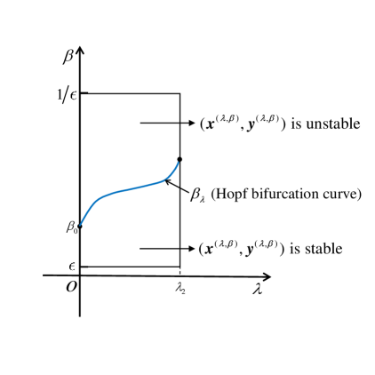
\lim_{\lambda\to 0}\frac{1}{\lambda}\left.\frac{d\mathcal{R}e[\mu(\beta)]}{d\beta}\right|_{\beta=\beta_{\lambda}}=\frac{1}{2}\sum_{j=1}^{n}b_{j}\xi_{j}>0.

∎

From Theorems 2.3, 3.3, 3.6 and 3.7, we can obtain the following results on the dynamics of model (1.5), see also Fig. 2.

Theorem 3.8.

Assume that $0<\epsilon\ll 1$ . Then there exists $\lambda_{2}>0$ (depending on $\epsilon$ ) and a continuously differentiable mapping

\lambda\mapsto\beta_{\lambda}:[0,\lambda_{2}]\to\mathcal{B}=[\epsilon,1/\epsilon]

such that, for each $\lambda\in(0,\lambda_{2}]$ , the positive equilibrium $(\bm{x}^{(\lambda,\beta)},\bm{y}^{(\lambda,\beta)})$ of model (1.5) is locally asymptotically stable when $\beta\in[\epsilon,\beta_{\lambda})$ and unstable when $\beta\in(\beta_{\lambda},\frac{1}{\epsilon}]$ . Moreover, system (1.5) undergoes a Hopf bifurcation at $(\bm{x}^{(\lambda,\beta)},\bm{y}^{(\lambda,\beta)})$ when $\beta=\beta_{\lambda}$ .

Proof.

Note from [16, Chapter 2, Theorem 5.1] that the eigenvalues of $A_{\beta}(\lambda)$ are continuous with respect to $\beta.$ We only need to show that there exists $\lambda_{2}>0$ , which depends on $\epsilon$ , such that

\sigma(A_{\beta}(\lambda))\subset\{x+{\rm i}y:x,y\in\mathbb{R},x<0\}\;\text{for}\;\lambda\in(0,\lambda_{2}]\;\text{and}\;\beta=\epsilon.

If it is not true, then there exists a sequence $\{\lambda_{l}\}_{l=1}^{\infty}$ such that $\lim_{l\to\infty}\lambda_{l}=0$ , and

\left(A_{\epsilon}({\lambda_{l}})-\mu I\right)(\bm{\varphi},\bm{\psi})^{T}=\bm{0}

(3.26)

is solvable for some value of $(\mu_{\lambda_{l}},\bm{\varphi}_{\lambda_{l}},\bm{\psi}_{\lambda_{l}})$ with $\mathcal{R}e\mu_{\lambda_{l}}\geq 0$ and $(\bm{\varphi}_{\lambda_{l}},\bm{\psi}_{\lambda_{l}})^{T}(\neq\bm{0})\in\mathbb{C}^{2n}$ . Here $A_{\epsilon}(\lambda_{l})=\left.A_{\beta}(\lambda_{l})\right|_{\beta=\epsilon}$ . Substituting $(\mu,\bm{\varphi},\bm{\psi})=(\mu_{\lambda_{l}},\bm{\varphi}_{\lambda_{l}},\bm{\psi}_{\lambda_{l}})$ into (3.26), we have

\begin{cases}\displaystyle\mu_{\lambda_{l}}\varphi_{{\lambda_{l}}j}=\sum_{k=1}^{n}p_{jk}\varphi_{{\lambda_{l}}k}+\lambda_{l}\left[M_{1j}^{({\lambda_{l}},\epsilon)}\varphi_{{\lambda_{l}}j}+M_{2j}^{({\lambda_{l}},\epsilon)}\psi_{{\lambda_{l}}j}\right],\;\;j=1,\dots,n,\\ \displaystyle\mu_{\lambda_{l}}\psi_{{\lambda_{l}}j}=\theta\sum_{k=1}^{n}q_{jk}\psi_{{\lambda_{l}}k}+\lambda_{l}\left[M_{3j}^{({\lambda_{l}},\epsilon)}\varphi_{{\lambda_{l}}j}-M_{2j}^{({\lambda_{l}},\epsilon)}\psi_{{\lambda_{l}}j}\right],\;\;j=1,\dots,n.\\ \end{cases}

(3.27)

Note from Lemma 3.1 that $\left|\mu_{\lambda_{l}}/{\lambda_{l}}\right|$ is bounded. Then, up to a subsequence, we assume that $\lim_{l\to\infty}\mu_{\lambda_{l}}/{\lambda_{l}}=\mu^{*}$ with $\mathcal{R}e\mu^{*}\geq 0$ . As in the proof of Lemma 3.5, we see that $(\bm{\varphi}_{\lambda l},\bm{\psi}_{\lambda l})^{T}(\neq\bm{0})\in\mathbb{C}^{2n}$ can be represented as

\begin{cases}\bm{\varphi}_{\lambda_{l}}=\delta_{\lambda_{l}}\bm{\xi}+\bm{w}_{\lambda_{l}},\;\;\text{where}\;\;\delta_{\lambda_{l}}\geq 0\;\;\text{and}\;\;\bm{w}_{\lambda_{l}}\in\mathcal{M}_{\mathbb{C}},\\ \bm{\psi}_{\lambda_{l}}=({s_{1}}_{\lambda_{l}}+{\rm i}{s_{2}}_{\lambda_{l}})\bm{\eta}+\bm{z}_{\lambda_{l}},\;\;\text{where}\;\;{s_{1}}_{\lambda_{l}},{s_{2}}_{\lambda_{l}}\in\mathbb{R}\;\;\text{and}\;\;\bm{z}_{\lambda_{l}}\in\mathcal{M}_{\mathbb{C}},\\ \|\bm{\varphi}_{\lambda_{l}}\|_{2}^{2}+\|\bm{\psi}_{\lambda_{l}}\|_{2}^{2}=\|\bm{\xi}\|_{2}^{2}+\|\bm{\eta}\|_{2}^{2},\end{cases}

(3.28)

and $\bm{w}_{\lambda_{l}}$ and $\bm{z}_{\lambda_{l}}$ satisfy

\lim_{l\to\infty}\bm{w}_{\lambda_{l}}=\bm{0},\;\;\lim_{l\to\infty}\bm{z}_{\lambda_{l}}=\bm{0}.

Up to a subsequence, we also assume that $\lim_{l\to\infty}\delta_{\lambda_{l}}=\delta^{*}$ , $\lim_{l\to\infty}{s_{1}}_{\lambda_{l}}=s_{1}^{*}$ and $\lim_{l\to\infty}{s_{2}}_{\lambda_{l}}=s_{2}^{*}$ . Dividing the first and second equation of (3.27) by $\lambda_{l}$ , respectively, summing the results over all $j$ , and taking the limits as $l\to\infty$ , we have

\begin{cases}\displaystyle\mu^{*}\delta^{*}=\delta^{*}\sum_{j=1}^{n}M_{1j}^{(0,\epsilon)}\xi_{j}+\left(s_{1}^{*}+{\rm i}s_{2}^{*}\right)\sum_{j=1}^{n}M_{2j}^{(0,\epsilon)}\eta_{j},\\ \displaystyle\mu^{*}\left(s_{1}^{*}+{\rm i}s_{2}^{*}\right)=\delta^{*}\sum_{j=1}^{n}M_{3j}^{(0,\epsilon)}\xi_{j}-\left(s_{1}^{*}+{\rm i}s_{2}^{*}\right)\sum_{j=1}^{n}M_{2j}^{(0,\epsilon)}\eta_{j}.\\ \end{cases}

It follows from (3.28) that at least one of $\delta^{*}$ and $s_{1}^{*}+{\rm i}s_{2}^{*}$ is not equal to zero. Consequently, $\mu^{*}$ is an eigenvalue of matrix

\left({\begin{array}[]{cc}\sum_{j=1}^{n}M_{1j}^{(0,\epsilon)}\xi_{j}&\sum_{j=1}^{n}M_{2j}^{(0,\epsilon)}\eta_{j}\\ \sum_{j=1}^{n}M_{3j}^{(0,\epsilon)}\xi_{j}&-\sum_{j=1}^{n}M_{2j}^{(0,\epsilon)}\eta_{j}\end{array}}\right).

It follows from (3.12) and (3.13) that, for sufficiently small $\epsilon$ ,

\sum_{j=1}^{n}M_{1j}^{(0,\epsilon)}\xi_{j}-\sum_{j=1}^{n}M_{2j}^{(0,\epsilon)}\eta_{j}<0,

which contradicts $\mathcal{R}e\mu^{*}\geq 0$ . This completes the proof. ∎

Noticing that model (1.5) is equivalent to the original model (1.3), we have the following result.

Theorem 3.9.

Assume that $0<\epsilon\ll 1$ , and $(\bf A_{1})-(\bf A_{2})$ hold. Then there exists $d_{*}>0$ (depending on $\epsilon$ ) and a continuously differentiable mapping

d_{1}\mapsto\beta^{d_{1}}:[d_{*},\infty)\to\mathcal{B}=[\epsilon,1/\epsilon]

such that, for each $d_{1}\in[d_{*},\infty)$ , the unique positive equilibrium of model (1.3) is locally asymptotically stable when $\beta\in[\epsilon,\beta^{d_{1}})$ and unstable when $\beta\in(\beta^{d_{1}},\frac{1}{\epsilon}]$ . Moreover, system (1.3) undergoes a Hopf bifurcation when $\beta=\beta^{d_{1}}$ .

4 The effect of the coupling matrices

In this section, we show the effect of the coupling matrices on the Hopf bifurcation value. Moreover, some numerical simulations are given to illustrate the theoretical results. For simplicity, we consider a special case, where $P=Q$ and the boxes are all identical (that is, $a_{i}=a$ and $b_{i}=1$ for $i=1,\dots,n$ ). Then, model (1.5) is reduced to the following form:

\begin{cases}\displaystyle\frac{dx_{j}}{dt}=\sum_{k=1}^{n}p_{jk}x_{k}+\lambda\left[a-(\beta+1)x_{j}+x_{j}^{2}y_{j}\right],&j=1,\dots,n,\;\;t>0,\\ \displaystyle\frac{dy_{j}}{dt}=\theta\sum_{k=1}^{n}p_{jk}y_{k}+\lambda\left(\beta x_{j}-x_{j}^{2}y_{j}\right),&j=1,\dots,n,\;\;t>0,\\ \bm{x}(0)=\bm{x}_{0}\geq(\not\equiv)\bm{0},\;\bm{y}(0)=\bm{y}_{0}\geq(\not\equiv)\bm{0}.\end{cases}

(4.1)

From Theorem 3.8, we have the following result on the dynamics of (4.1).

Proposition 4.1.

Assume that $0<\epsilon\ll 1$ . Then there exists $\lambda_{2}>0$ (depending on $\epsilon$ ) and a Hopf bifurcation curve:

\lambda\mapsto\beta_{\lambda}:[0,\lambda_{2}]\to\mathcal{B}=[\epsilon,1/\epsilon]

such that, for each $\lambda\in(0,\lambda_{2}]$ , the positive equilibrium $(\bm{x}^{(\lambda,\beta)},\bm{y}^{(\lambda,\beta)})$ of system (4.1) is locally asymptotically stable when $\beta\in[\epsilon,\beta_{\lambda})$ and unstable when $\beta\in(\beta_{\lambda},\frac{1}{\epsilon}]$ . Moreover, system (4.1) undergoes a Hopf bifurcation at $(\bm{x}^{(\lambda,\beta)},\bm{y}^{(\lambda,\beta)})$ when $\beta=\beta_{\lambda}$ , and $\beta_{\lambda}$ satisfies

\lim_{\lambda\to 0}\beta_{\lambda}=\beta_{0}=1+(na)^{2}\left(\sum_{j=1}^{n}\xi_{j}^{3}\right),

(4.2)

where $(\xi_{1},\dots,\xi_{n})$ satisfying (1.4) is the corresponding eigenfunction of $P$ with respect to eigenvalue $0$ .

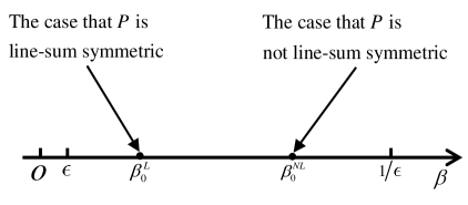
Now, we show the effect of the coupling matrix on the Hopf bifurcation value. We recall the $P=(p_{jk})$ is line-sum symmetric matrix if $\sum_{k\neq j}p_{jk}=\sum_{k\neq j}p_{kj}$ for all $j=1,\dots,n$ .

Proposition 4.2.

Denote $\beta_{0}$ by $\beta_{0}^{L}$ (respectively, $\beta_{0}^{NL}$ ) when $P=(p_{jk})$ is line-sum symmetric (respectively, not line-sum symmetric). Then $\beta_{0}^{L}<\beta_{0}^{NL}$ .

Proof.

It follows from (4.2) that $\beta_{0}=1+(na)^{2}\left(\sum_{j=1}^{n}\xi_{j}^{3}\right)$ . A direct computation implies that

\bm{\xi}=(\xi_{1},\dots,\xi_{n})^{T}=\left(\frac{1}{n},\dots,\frac{1}{n}\right)^{T},

if and only if $P$ is line-sum symmetric. Then we see that $\beta_{0}^{L}=1+a^{2}$ . It follows from (1.4) and Hölder inequality that

1=\left(\sum_{j=1}^{n}\xi_{j}\right)^{3}\leq\left(\sum_{j=1}^{n}1^{\frac{3}{2}}\right)^{2}\left(\sum_{j=1}^{n}\xi_{j}^{3}\right)=n^{2}\left(\sum_{j=1}^{n}\xi_{j}^{3}\right),

(4.3)

and the equality holds if and only if $\xi_{j}=1/n$ for $j=1\cdots n$ . Then, we see from (4.2) and (4.3) that $\beta_{0}^{L}<\beta_{0}^{NL}$ . ∎

From Propositions 4.1 and 4.2, we see that the Hopf bifurcation value with line-sum symmetric coupling matrix is smaller than that for the non-line-sum symmetric case, see Fig. 3.

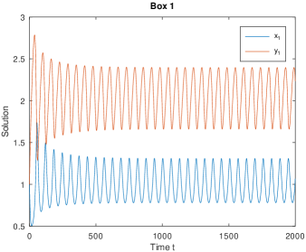
This phenomenon can also be illustrated numerically. We consider model (4.1), and choose the parameters and initial values as follows:

n=3,\;\;\beta=2.05,\;\;\lambda=0.1,\;\;\theta=1,\;\;a=1,\;\;x_{j}(0)=y_{j}(0)=1,(j=1,2,3).

Here we choose two different coupling matrices:

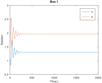
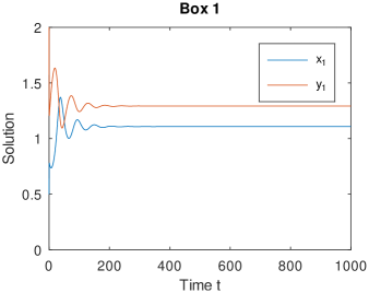
P^{L}:=\left({\begin{array}[]{ccc}-2&1&1\\ 1&-3&2\\ 1&2&-3\end{array}}\right),\;\;P^{NL}:=\left({\begin{array}[]{ccc}-3&2&3\\ 2&-3&2\\ 1&1&-5\end{array}}\right),

where $P^{L}$ is line-sum symmetric, and $P^{NL}$ is not line-sum symmetric. Then when $\beta(=2.05)$ is fixed, model (4.1) admits a positive periodic solution for $P=P^{L}$ , while the positive equilibrium is stable for $P=P^{NL}$ , see Fig. 4. This shows that the Hopf bifurcation value of model (4.1) for $P=P^{L}$ is smaller than that for $P=P^{NL}$ .

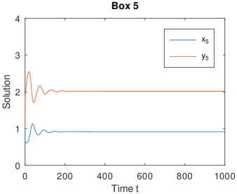
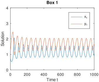
Finally, we provide some numerical simulations to illustrate the theoretical results obtained in Section 3. Here we consider model (1.5), and choose $n=5$ , $\lambda=0.1$ , $\theta=1$ and coupling matrices:

P:=\left({\begin{array}[]{ccccc}-4&1&1&1&1\\ 1&-5&2&1&1\\ 1&1&-5&1&1\\ 1&2&1&-4&2\\ 1&1&1&1&-5\end{array}}\right),\;\;Q:=\left({\begin{array}[]{ccccc}-5&1&1&1&1\\ 1&-6&2&1&1\\ 1&1&-5&1&1\\ 2&1&1&-6&3\\ 1&3&1&3&-6\end{array}}\right).

Moreover, let $\beta$ be the variable parameter and choose the other parameters as Table 1.

Table 1: Initial concentrations of reactants in five boxes.

	1	2	3	4	5
$a_{j}$	1	2	1	0.5	1
$b_{j}$	0.1	0.2	0.4	0.1	0.2
$x_{j}(0)$	0.5	1	1	0.5	1
$y_{j}(0)$	2	1	2	1	1

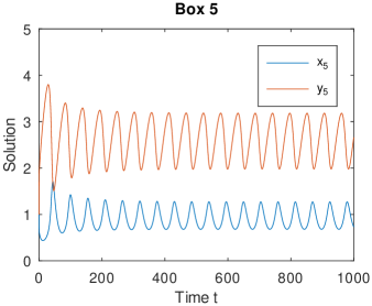
We numerically show that model (1.5) can undergoes a Hopf bifurcation, and consequently periodic solutions can arise, see Figs. 5 and 6.

Statements and Declarations

Funding: This study was funded by National Natural Science Foundation of China (grant number 12171117) and Shandong Provincial Natural Science Foundation of China (grant number ZR2020YQ01).
Conflict of Interest: The authors declare that they have no conflict of interest. Availability of date and materials: All data generated or analysed during this study are included in this published article.

References

[1] Q. An, C. Wang, and H. Wang. Analysis of a spatial memory model with nonlocal maturation delay and hostile boundary condition. Discrete Contin. Dyn. Syst., 40(10):5845–5868, 2020.
[2] P. Andresen, M. Bache, E. Mosekilde, G. Dewel, and P. Borckmans. Stationary space-periodic structures with equal diffusion coefficients. Phys. Rev. E, 60(1):297–301, 1999.
[3] K. J. Brown and F. A. Davidson. Global bifurcation in the Brusselator system. Nonlinear Anal., 24(12):1713–1725, 1995.
[4] S. Busenberg and W. Huang. Stability and Hopf bifurcation for a population delay model with diffusion effects. J. Differential Equations, 124(1):80–107, 1996.
[5] S. Chen, Y. Lou, and J. Wei. Hopf bifurcation in a delayed reaction-diffusion-advection population model. J. Differential Equations, 264(8):5333–5359, 2018.
[6] S. Chen and J. Shi. Stability and Hopf bifurcation in a diffusive logistic population model with nonlocal delay effect. J. Differential Equations, 253(12):3440–3470, 2012.
[7] Y. Choi, T. Ha, J. Han, S. Kim, and D. S. Lee. Turing instability and dynamic phase transition for the Brusselator model with multiple critical eigenvalues. Discrete Contin. Dyn. Syst., 41(9):4255–4281, 2021.
[8] M. Duan, L. Chang, and Z. Jin. Turing patterns of an SI epidemic model with cross-diffusion on complex networks. Phys. A, 533:122023, 2019.
[9] R. J. Field and R. M. Noyes. Oscillations in chemical systems. IV. Limit cycle behavior in a model of a real chemical reaction. J. Chem. Phys., 60(5):1877–1884, 1974.
[10] G. Guo, J. Wu, and X. Ren. Hopf bifurcation in general Brusselator system with diffusion. Appl. Math. Mech. (English Ed.), 32(9):1177–1186, 2011.
[11] S. Guo. Stability and bifurcation in a reaction-diffusion model with nonlocal delay effect. J. Differential Equations, 259(4):1409–1448, 2015.
[12] S. Guo and S. Yan. Hopf bifurcation in a diffusive Lotka-Volterra type system with nonlocal delay effect. J. Differential Equations, 260(1):781–817, 2016.
[13] R. Hu and Y. Yuan. Spatially nonhomogeneous equilibrium in a reaction-diffusion system with distributed delay. J. Differential Equations, 250(6):2779–2806, 2011.
[14] Y. Jia, Y. Li, and J. Wu. Coexistence of activator and inhibitor for Brusselator diffusion system in chemical or biochemical reactions. Appl. Math. Lett., 53:33–38, 2016.
[15] Z. Jin and R. Yuan. Hopf bifurcation in a reaction-diffusion-advection equation with nonlocal delay effect. J. Differential Equations, 271:533–562, 2021.
[16] T. Kato. Perturbation theory in a finite-dimensional space. Springer Berlin Heidelberg, 1995.
[17] Y. Kuramoto. Chemical oscillations, waves, and turbulence, volume 19 of Springer Series in Synergetics. Springer Berlin Heidelberg, 1984.
[18] S. P. Kuznetsov. Noise-induced absolute instability. Math. Comput. Simulation, 58(4-6):435–442, 2002.
[19] R. Lefever and G. Nicolis. Chemical instabilities and sustained oscillations. J. Theor. Biol., 30(2):267–284, 1971.
[20] I. Lengyel and I. R. Epstein. Diffusion-induced instability in chemically reacting systems: steady-state multiplicity, oscillation, and chaos. Chaos, 1(1):69–76, 1991.
[21] B. Li and M. Wang. Diffusion-driven instability and Hopf bifurcation in Brusselator system. Appl. Math. Mech. (English Ed.), 29(6):825–832, 2008.
[22] Q.-S. Li and J.-C. Shi. Cooperative effects of parameter heterogeneity and coupling on coherence resonance in unidirectional coupled brusselator system. Phys. Lett. A, 360(4):593–598, 2007.
[23] Y. Li. Hopf bifurcations in general systems of Brusselator type. Nonlinear Anal. Real World Appl., 28:32–47, 2016.
[24] Z. Li and B. Dai. Stability and Hopf bifurcation analysis in a Lotka-Volterra competition-diffusion-advection model with time delay effect. Nonlinearity, 34(5):3271–3313, 2021.
[25] M. Liao and Q.-R. Wang. Stability and bifurcation analysis in a diffusive Brusselator-type system. Internat. J. Bifur. Chaos Appl. Sci. Engrg., 26(7):1650119, 11, 2016.
[26] M. Ma and J. Hu. Bifurcation and stability analysis of steady states to a Brusselator model. Appl. Math. Comput., 236:580–592, 2014.
[27] R. Peng and M. Wang. Pattern formation in the Brusselator system. J. Math. Anal. Appl., 309(1):151–166, 2005.
[28] R. Peng and M. Yang. On steady-state solutions of the Brusselator-type system. Nonlinear Anal., 71(3-4):1389–1394, 2009.
[29] J. Petit, M. Asllani, D. Fanelli, B. Lauwens, and T. Carletti. Pattern formation in a two-component reaction-diffusion system with delayed processes on a network. Phys. A, 462:230–249, 2016.
[30] I. Prigogine and R. Lefever. Symmetry breaking instabilities in dissipative systems. II. J. Chem. Phys., 48(4):1695–1700, 1968.
[31] I. Schreiber, M. Holodniok, M. Kubíček, and M. Marek. Periodic and aperiodic regimes in coupled dissipative chemical oscillators. J. Statist. Phys., 43(3-4):489–519, 1986.
[32] J.-C. Shi and Q.-S. Li. The enhancement and sustainment of coherence resonance in a two-way coupled brusselator system. Phys. D, 225(2):229–234, 2007.
[33] H. L. Smith. Monotone dynamical systems: an introduction to the theory of competitive and cooperative systems: an introduction to the theory of competitive and cooperative systems, volume 41. American Mathematical Society, 1995.
[34] Y. Su, J. Wei, and J. Shi. Hopf bifurcations in a reaction-diffusion population model with delay effect. J. Differential Equations, 247(4):1156–1184, 2009.
[35] C. Tian and S. Ruan. Pattern formation and synchronism in an allelopathic plankton model with delay in a network. SIAM J. Appl. Dyn. Syst., 18(1):531–557, 2019.
[36] R. W. Wittenberg and P. Holmes. The limited effectiveness of normal forms: a critical review and extension of local bifurcation studies of the Brusselator PDE. Phys. D, 100(1-2):1–40, 1997.
[37] X.-P. Yan and W.-T. Li. Stability of bifurcating periodic solutions in a delayed reaction-diffusion population model. Nonlinearity, 23(6):1413–1431, 2010.
[38] X.-P. Yan and W.-T. Li. Stability and Hopf bifurcations for a delayed diffusion system in population dynamics. Discrete Contin. Dyn. Syst. Ser. B, 17(1):367–399, 2012.
[39] X.-P. Yan, P. Zhang, and C.-H. Zhang. Turing instability and spatially homogeneous Hopf bifurcation in a diffusive Brusselator system. Nonlinear Anal. Model. Control, 25(4):638–657, 2020.
[40] P. Yu and A. B. Gumel. Bifurcation and stability analyses for a coupled Brusselator model. J. Sound Vibration, 244(5):795–820, 2001.