Holographic thermodynamic relation for dissipative and non-dissipative universes
in a flat FLRW cosmology
Abstract
Horizon thermodynamics and cosmological equations in standard cosmology provide a holographic-like connection between thermodynamic quantities on a cosmological horizon and in the bulk. It is expected that this connection can be modified as a holographic-like thermodynamic relation for dissipative and non-dissipative universes whose Hubble volume varies with time . To clarify such a modified thermodynamic relation, the present study applies a general formulation for cosmological equations in a flat Friedmann–Lemaître–Robertson–Walker (FLRW) universe to the first law of thermodynamics, using the Bekenstein–Hawking entropy and a dynamical Kodama–Hayward temperature . For the general formulation, both an effective pressure of cosmological fluids for dissipative universes (e.g., bulk viscous cosmology) and an extra driving term for non-dissipative universes (e.g., time-varying cosmology) are phenomenologically assumed. A modified thermodynamic relation is derived by applying the general formulation to the first law, which includes both and an additional time-derivative term , related to a non-zero term of the general continuity equation. When is constant, the modified thermodynamic relation is equivalent to the formulation of the first law in standard cosmology. One side of this modified relation describes thermodynamic quantities in the bulk and can be divided into two time-derivative terms, namely and terms, where is the mass density of cosmological fluids. Using the Gibbons–Hawking temperature , the other side of this relation, , can be formulated as the sum of and , which are equivalent to the and terms, respectively, with the magnitude of the term being proportional to the square of the term. In addition, the modified thermodynamic relation for constant is examined by applying the equipartition law of energy on the horizon. This modified thermodynamic relation reduces to a kind of extended holographic-like connection when a constant universe (whose Hubble volume varies with time) is considered. The evolution of thermodynamic quantities is also discussed, using a constant model, extending a previous analysis [N. Komatsu, Phys. Rev. D 108, 083515 (2023)].
pacs:
98.80.-k, 95.30.TgI Introduction
To explain the accelerated expansion of the late Universe PERL1998_Riess1998 ; Planck2018 ; Hubble2017 , astrophysicists have proposed various cosmological models, e.g., lambda cold dark matter (CDM) models, time-varying cosmology FreeseOverduin ; Nojiri2006etc ; Valent2015Sola2019 ; Sola_2009-2022 , creation of CDM (CCDM) models Prigogine_1988-1989 ; Lima1992-1996 ; LimaOthers2023 ; Freaza2002Cardenas2020 , bulk viscous cosmology BarrowLima ; BrevikNojiri ; EPJC2022 , and thermodynamic scenarios such as entropic cosmology EassonCai ; Basilakos1 ; Koma45 ; Koma6 ; Koma7 ; Koma8 ; Koma9 ; Neto2022 ; Gohar2024 . These studies imply that our Universe should finally approach a de Sitter universe whose horizon is considered to be in thermal equilibrium. The thermodynamics of the universe has been examined from various perspectives, e.g., the first law of thermodynamics Cai2005 ; Cai2011 ; Dynamical-T-2007 ; Dynamical-T-20092014 ; Sheykhi1 ; Sheykhi2Karami ; Santos2022 ; Sheykhia2018 ; ApparentHorizon2022 ; Cai2007 ; Cai2007B ; Cai2008 ; Sanchez2023 ; Nojiri2024 ; Odintsov2023ab ; Odintsov2024 ; Mohammadi2023 ; Odintsov2024B , the second law of thermodynamics Easther1-Egan1 ; Pavon2013Mimoso2013 ; Bamba2018Pavon2019 ; deSitter_entropy ; Saridakis2019 ; Saridakis2021 ; Sharif2024 , and the holographic equipartition law related to the emergence of cosmic space Padma2010 ; Verlinde1 ; HDE ; Padmanabhan2004 ; ShuGong2011 ; Koma14 ; Koma15 ; Koma16 ; Koma17 ; Koma19 ; Koma20 ; Padma2012AB ; Cai2012 ; Hashemi ; Moradpour ; Wang ; Koma10 ; Koma11 ; Koma12 ; Koma18 ; Krishna20172019 ; Mathew2022 ; Chen2022 ; Luciano ; Mathew2023 ; Mathew2023b ; Pad2017 ; Tu2018 ; Tu2019 ; Chen2024 .
In the thermodynamic scenarios, black hole thermodynamics Hawking1Bekenstein1 is applied to a cosmological horizon and the information of the bulk is assumed to be stored on the horizon, based on the holographic principle Hooft-Bousso . In particular, the first law of thermodynamics has been examined from a holographic viewpoint Cai2005 ; Cai2011 ; Dynamical-T-2007 ; Dynamical-T-20092014 ; Sheykhi1 ; Sheykhi2Karami ; Santos2022 ; Sheykhia2018 ; ApparentHorizon2022 ; Cai2007 ; Cai2007B ; Cai2008 ; Sanchez2023 ; Nojiri2024 ; Odintsov2023ab ; Odintsov2024 ; Mohammadi2023 ; Odintsov2024B . In these works (excepting Refs. Santos2022 ; Mohammadi2023 ), the Friedmann equation is derived from the first law, using the continuity equation whose right-hand side is considered to be zero. Of course, it is well known that the continuity equation can be non-zero in cosmological models for both dissipative universes (e.g., bulk viscous models) and non-dissipative universes (e.g., CDM models) Koma9 . In fact, a general formulation for the cosmological equations of the two types of universes has been examined in previous works Koma9 ; Koma16 . We expect that a holographic thermodynamic relation for dissipative and non-dissipative universes can be derived by applying the general formulation to the first law of thermodynamics.
In addition, Padmanabhan Pad2017 has derived an energy-balance relation using the equipartition law of energy on the horizon. A similar holographic-like connection relation has been recently examined Koma18 , where is an energy in the bulk and is the Helmholtz free energy on the horizon. (For details on the holographic-like connection, see Appendix A and Ref. Koma18 .) In these works, de Sitter universes are originally considered and, therefore, the Hubble parameter, the Hubble volume, and the Gibbons–Hawking temperature GibbonsHawking1977 are constant. In a de Sitter universe, is equivalent to the dynamical Kodama–Hayward temperature Dynamical-T-2007 ; Dynamical-T-20092014 , based on the works of Hayward et al. Dynamical-T-1998 ; Dynamical-T-2008 . Of course, the horizons of universes are generally considered to be dynamic, unlike for de Sitter universes. Accordingly, a dynamical temperature should be appropriate for discussing the thermodynamics on a dynamic horizon Koma19 .
The first law of thermodynamics has been recently examined using the dynamical Kodama–Hayward temperature . (For the first law, see the previous works of Akbar and Cai Cai2007 ; Cai2007B and Cai et al. Cai2008 and recent works of Sánchez and Quevedo Sanchez2023 , Nojiri et al. Nojiri2024 , and Odintsov et al. Odintsov2023ab ; Odintsov2024 ; Odintsov2024B .) The first law should lead to an extended holographic-like connection, namely a modified thermodynamic relation for dissipative and non-dissipative universes whose Hubble volume varies with time. We expect that the thermodynamic relation between the horizon and the bulk can reduce to a simple relation similar to the holographic-like connection by applying the equipartition law of energy on the horizon.
However, the modified thermodynamic relation has not yet been discussed from those viewpoints. An understanding of the thermodynamic relation for dissipative and non-dissipative universes should provide new insights into the thermodynamics on the horizon and cosmological equations in the bulk. In this context, we examine the thermodynamic relation by applying a general formulation for cosmological equations to the first law of thermodynamics.
The remainder of the present article is organized as follows. In Sec. II, a general formulation for cosmological equations is reviewed. In addition, an associated entropy and an approximate temperature on a cosmological horizon are introduced. In Sec. III, the general formulation is applied to the first law of thermodynamics to derive a modified thermodynamic relation. In Sec. IV, the modified thermodynamic relation is discussed under a specific condition. In Sec. IV.1, the left-hand side of the modified thermodynamic relation, corresponding to thermodynamic quantities in the bulk, is examined. In Sec. IV.2, the equipartition law of energy on the horizon is applied to the right-hand side of the relation, namely thermodynamic quantities on the horizon. In Sec. V, typical evolutions of the thermodynamic quantities in the relation are observed using cosmological models. Finally, in Sec. VI, the conclusions of the study are presented.
In this paper, a homogeneous, isotropic, and spatially flat universe, namely a flat Friedmann–Lemaître–Robertson–Walker (FLRW) universe, is considered. Therefore, the apparent horizon of the universe is equivalent to the Hubble horizon. Also, an expanding universe is assumed from observations Hubble2017 . Inflation of the early universe and density perturbations related to structure formations are not discussed.
II Cosmological equations, horizon entropy, and horizon temperature
In the present study, a general formulation for cosmological equations is applied to the first law of thermodynamics. For this, Sec. II.1 reviews the general formulation, while in Sec. II.2, the Bekenstein–Hawking entropy, the Gibbons–Hawking temperature, and a dynamical Kodama–Hayward temperature on the Hubble horizon are introduced.
II.1 General formulation for cosmological equations in a flat FLRW universe
We introduce a general formulation for cosmological equations in dissipative and non-dissipative universes, using the scale factor at time , based on previous works Koma6 ; Koma9 ; Koma14 ; Koma15 ; Koma16 . The general Friedmann, acceleration, and continuity equations are written as
| (1) |
| (2) |
| (3) |
with the Hubble parameter defined as
| (4) |
where , , , and are the gravitational constant, the speed of light, the mass density of cosmological fluids, and the pressure of cosmological fluids, respectively. Two extra driving terms, and , are phenomenologically assumed Koma14 . Specifically, is used for a model, similar to CDM models, whereas is used for a BV (bulk-viscous-cosmology-like) model, similar to bulk viscous models and CCDM models Koma14 ; Koma16 . That is, is used for non-dissipative universes and is used for dissipative universes. In this study, and are considered simultaneously. Only two of the three equations (the Friedmann, acceleration, and continuity equations) are independent Ryden1 . Therefore, the general continuity equation given by Eq. (3) can be derived from Eqs. (1) and (2). In addition, subtracting Eq. (1) from Eq. (2) yields
| (5) |
These equations are used in Sec. III.
Equation (3) indicates that the right-hand side of the general continuity equation is non-zero. A similar non-zero term appears in other cosmological models, such as energy exchange cosmology Barrow22 ; Wang0102 ; Dynamical20052013 and the bulk viscous and CCDM models Prigogine_1988-1989 ; Lima1992-1996 ; LimaOthers2023 ; Freaza2002Cardenas2020 ; BarrowLima ; BrevikNojiri ; EPJC2022 , as discussed in Refs. Koma9 ; Koma20 . For example, energy exchange cosmology assumes the transfer of energy between two fluids Barrow22 , such as the interaction between dark matter and dark energy Wang0102 . In this case, the two non-zero right-hand sides are totally cancelled because the total energy of the two fluids is conserved Koma20 . In the bulk viscous and CCDM models, an effective formulation can be obtained from an effective description for pressure, using a single fluid, as examined in the next paragraph. (When , the general cosmological equations reduce to those for standard cosmology and, therefore, the continuity equation is given by . The same continuity equation can be obtained when both and are considered, as for CDM models.)
We now consider an effective formulation, using an effective pressure, , which is given by Koma9
| (6) |
where has been replaced by . Applying the effective pressure to Eqs. (2), (3), and (5) yields Koma9
| (7) |
| (8) |
| (9) |
where includes the term. The effective pressure can be related to irreversible entropies because the term is considered to be related to an irreversible entropy arising from dissipative processes, such as the bulk viscosity Koma7 . The effective formulation is used in Sec. III. The right-hand side of Eq. (8) is non-zero except when . This non-zero term affects the modified thermodynamics relation and is examined in Sec. III. The Friedmann equation for the effective formulation is given by Eq. (1), because the Friedmann equation does not include .
It should be noted that coupling Eq. (1) with Eq. (2) yields the cosmological equation Koma14 ; Koma15 ; Koma16 , given by
| (10) |
where represents the equation of the state parameter for a generic component of matter, which is given as . For a matter-dominated universe and a radiation-dominated universe, the values of are and , respectively. Instead of , is used for because Eq. (10) includes . Equation (10) can describe background evolutions of the universe in various cosmological models Koma14 ; Koma15 ; Koma16 . Accordingly, Eq. (10) is used for the discussion of cosmological models, such as a constant model Koma19 , as examined later.
II.2 Entropy and temperature on the horizon
The horizon thermodynamics is closely related to the holographic principle Hooft-Bousso , which assumes that the horizon of the universe has an associated entropy and an approximate temperature EassonCai . The entropy and the temperature on the Hubble horizon are introduced according to previous works Koma11 ; Koma12 ; Koma17 ; Koma18 ; Koma19 ; Koma20 .
We select the Bekenstein–Hawking entropy as the associated entropy because it is the most standard. In general, the cosmological horizon is examined by replacing the event horizon of a black hole by the cosmological horizon Koma17 ; Koma18 . This replacement method has been widely accepted Jacob1995; Padma2010 ; Verlinde1 ; HDE ; Padma2012AB ; Cai2012 ; Moradpour ; Hashemi ; Wang ; Padmanabhan2004 ; ShuGong2011 ; Koma14 ; Koma15 ; Koma16 ; Koma17 ; Koma19 ; Koma20 and we use it here.
Based on the form of the Bekenstein–Hawking entropy, the entropy is written as Hawking1Bekenstein1
| (11) |
where and are the Boltzmann constant and the reduced Planck constant, respectively. The reduced Planck constant is defined by , where is the Planck constant Koma11 ; Koma12 . is the surface area of the sphere with a Hubble horizon (radius) given by
| (12) |
Substituting into Eq. (11) and applying Eq. (12) yields
| (13) |
where is a positive constant given by
| (14) |
When a de Sitter universe is considered, is constant although the scale factor exponentially increases with time. Differentiating Eq. (13) with respect to yields the first derivative of , given by Koma11 ; Koma12
| (15) |
The second law of thermodynamics on the horizon, , is satisfied in favored cosmological models, such as CDM models Koma14 . In the present study, the form of the Bekenstein–Hawking entropy, , is typically used for the entropy on the cosmological horizon. (Various forms of black-hole entropy such as nonextensive entropy have been proposed Das2008 ; Radicella2010 ; LQG2004_123 ; Tsallis2012 ; Czinner1Czinner2 ; Barrow2020 ; Nojiri2022 ; Gohar2023 , as described in Refs. Koma18 ; Koma19 ; Koma20 . For a general form of entropy related to the Friedmann equation, see, e.g., Ref. Nojiri2024 .)
Next, we introduce an approximate temperature on the Hubble horizon. Before introducing a dynamical temperature, we review the Gibbons–Hawking temperature , which is given by GibbonsHawking1977
| (16) |
This equation indicates that is proportional to and is constant during the evolution of de Sitter universes Koma17 ; Koma19 . In fact, is obtained from field theory in the de Sitter space GibbonsHawking1977 . However, most universes are not pure de Sitter universes in that their horizons are dynamic. That is, horizons of universes (including our Universe) are generally considered to be dynamic Koma19 ; Koma20 . Therefore, we introduce a dynamical Kodama–Hayward temperature, based on a previous work Koma19 .
In fact, a similar dynamic horizon for black holes has been examined in the works of Hayward Dynamical-T-1998 and Hayward et al. Dynamical-T-2008 , as described in Ref. Koma19 . Hayward suggested a dynamical temperature on a black hole horizon and clarified the relationship between the surface gravity and the temperature on a dynamic apparent horizon for the Kodama observer Dynamical-T-1998 . The Kodama–Hayward temperature on the cosmological horizon of an FLRW universe has been proposed Dynamical-T-2007 ; Dynamical-T-20092014 , based on the works of Hayward et al. Dynamical-T-1998 ; Dynamical-T-2008 .
The Kodama–Hayward temperature for a flat FLRW universe can be written as Tu2018 ; Tu2019
| (17) |
Here and are assumed for a non-negative temperature in an expanding universe Koma19 ; Koma20 . When de Sitter universes are considered, reduces to because and, therefore, is interpreted as an extended version of Koma19 ; Koma20 . In the present paper, the Kodama–Hayward temperature is typically used for the temperature on the horizon. Cosmological models used later satisfy a non-negative temperature.
As examined in Refs. Koma19 ; Koma20 , is constant when the following equation is satisfied:
| (18) |
where represents a dimensionless constant. Substituting Eq. (18) into Eq. (17) gives a constant temperature, Koma19 ; Koma20 . Accordingly, is non-negative when is considered in an expanding universe. A universe at constant has been studied, using a cosmological model which includes a power-law term proportional to (where is a free variable) and the equation of state parameter Koma19 ; Koma20 . For example, substituting , , and into Eq. (10) yields the cosmological equation equivalent to Eq. (18). (The term for is obtained from when .) In this universe, is constant though the Hubble parameter varies with time. Understanding the universe at constant should contribute to the study of horizon thermodynamics because systems at constant temperature play important roles in thermodynamics. In Sec. IV.2, we consider a constant universe, to simplify the modified thermodynamic relation. In Sec. V, the evolution of the constant universe is observed, using a constant model. To formulate the constant model, a power-law model with terms is discussed in Sec. V.
III First law of thermodynamics and the modified thermodynamic relation
In this section, we derive the modified thermodynamic relation by applying the general formulation for cosmological equations to the first law of thermodynamics. For this, we review the first law according to Refs. Cai2007 ; Cai2007B ; Cai2008 ; Sanchez2023 ; Nojiri2024 ; Odintsov2023ab ; Odintsov2024 ; Odintsov2024B . In the present paper, a flat FLRW universe is considered and, therefore, the Hubble horizon is equivalent to an apparent horizon.
The first law of thermodynamics is written as Cai2007 ; Cai2007B ; Cai2008 ; Sanchez2023 ; Nojiri2024 ; Odintsov2023ab ; Odintsov2024 ; Odintsov2024B
| (21) |
where is the total internal energy of the matter fields inside the horizon, given by
| (22) |
represents the work density done by the matter fields Nojiri2024 , which is written as
| (23) |
and is the Hubble volume, written as
| (24) |
where given by Eq. (12) is used. Equation (21) indicates that the entropy on the horizon is generated, based on both the decreasing total internal energy of the bulk () and the work done by the matter fields () Nojiri2024 . The right-hand side of Eq. (21) should correspond to thermodynamic quantities on the horizon and may be modified as , using an effective entropy Cai2007B , as discussed later. In contrast, the left-hand side may be related to be the energy flux of matter fields from inside to outside the horizon for an infinitesimal time, as described in Ref. Nojiri2024 . The work density given by Eq. (23) is based on the fact that the work done is obtained by the trace of the energy-momentum tensor of the matter fields along the direction perpendicular to the (apparent) horizon Odintsov2024B . We note that an alternative work density is discussed in Ref. Nojiri2024 .
In addition, Eq. (21) can be written as
| (25) |
or equivalently,
| (26) |
The left-hand side describes thermodynamic quantities in the bulk, whereas the right-hand side describes thermodynamic quantities on the horizon. Originally, and were considered Cai2007 and the first law is satisfied in standard cosmology.
In this study, we typically use and . However, and are retained so that we can consider other entropies and temperatures. For example, when nonextensive entropies Das2008 ; Radicella2010 ; LQG2004_123 ; Tsallis2012 ; Czinner1Czinner2 ; Barrow2020 ; Nojiri2022 ; Gohar2023 are used for , the first law of thermodynamics should lead to the modified Friedmann and acceleration equations, as examined in previous works; see, e.g., Ref. Odintsov2024 . Also, a general form of entropy has been discussed based on the first law Nojiri2024 .
We examine Eq. (26) and calculate the left-hand side of this equation. Substituting Eqs. (22) and (23) into yields Nojiri2024
| (27) |
The above equation indicates that is divided into a term and a term, namely and . Hereafter we call the two terms the ‘ and terms’, even when is replaced by . This result implies that can also be divided into two parts, corresponding to the and terms. This consistency is examined in Sec. IV.1. Note that the term is the sum of and .
We now apply general cosmological equations to the first law of thermodynamics. Equation (27) corresponds to the left-hand side of Eq. (26). and in Eq. (27) are calculated using Eqs. (3) and (5). Substituting Eqs. (3) and (5) into Eq. (27), applying given by Eq. (24) and , and performing several operations yields
| (28) |
where given by Eq. (20) is also used. Equation (28) corresponds to the left-hand side of Eq. (26). Therefore, from Eq. (28), the first law based on Eq. (26) may be written as
| (29) |
where represents an effective entropy Cai2007B . In this study, is assumed to be given by
| (30) |
where and represent reversible and irreversible entropies, which are related to the additional and terms in the first line of Eq. (29), respectively. Equation (29) is considered to be a generalized first law of thermodynamics. We call this a ‘modified thermodynamic relation’, because Eq. (29) has not yet been established. We can confirm that when , Eq. (29) reduces to , where is also used.
The additional and terms in Eq. (29) are based on two extra driving terms included in general cosmological equations, and these two terms are assumed to be related to entropies. In this paper, the term is considered to be related to the reversible entropy , such as that related to the reversible exchange of energy. The term is considered to be related to the irreversible entropy arising from dissipative processes, such as the bulk viscosity and the creation of CDM Koma7 . Other entropies, such as nonequilibrium entropies and generalized entropies, are not considered here. The relationship between similar additional terms and nonequilibrium entropies has been discussed in, e.g., Refs. Dynamical-T-2007 ; Cai2007B ; Santos2022 . A general form of entropy that connects the Friedmann equations for any gravity theory with horizon thermodynamics has been examined in Ref. Nojiri2024 . We expect that modified FLRW equations can be derived from Eq. (29), using various forms of entropy on the horizon Das2008 ; Radicella2010 ; LQG2004_123 ; Tsallis2012 ; Czinner1Czinner2 ; Barrow2020 ; Nojiri2022 ; Gohar2023 . The modified thermodynamic relation given by Eq. (29) should provide new insights into thermodynamics and cosmological equations.
For an effective formulation, we apply an effective pressure given by Eq. (6) to the modified thermodynamic relation. Using , Eq. (29) can be written as
| (31) |
where is the effective work density, given by
| (32) |
Equation (31) is also a ‘modified thermodynamic relation’. includes the effect of . The additional and terms should lead to modified cosmological equations and may be related to a corrected term for a generalized entropy. These tasks are left for future research. Hereafter, we consider a constant and neglect the additional terms. Substituting into Eq. (31) yields
| (33) |
where has been also used. This simplified relation implicitly includes and a constant , corresponding to a cosmological constant. Equation (33) has not yet been established, but it is consistent with the formulation of the first law given by Eq. (26). When , this relation is equivalent to the first law itself, because . In fact, Eq. (33) is expected to provide significant information even though the additional terms are neglected. Therefore, we examine Eq. (33) in the next section.
IV Modified thermodynamic relation for constant
In this section, we examine the modified thermodynamic relation for constant . That is, we consider a constant and an effective pressure . From Eq. (33), the modified thermodynamic relation is written as
| (34) |
or equivalently,
| (35) |
where is the effective work density , given by Eq. (32). The above two equations are the modified thermodynamic relation examined in this section. The left-hand sides of the two equations describe thermodynamic quantities in the bulk, while the middles and the right-hand sides describe thermodynamic quantities on the horizon. In and , the subscript indicates thermodynamic quantities on the horizon, as examined below.
The Helmholtz free energy is defined as Callen and, therefore, is given by . Accordingly, and are written as
| (36) |
Applying Eq. (36) to the right-hand side of Eqs. (34) and (35) yields the modified thermodynamic relation:
| (37) |
| (38) |
where and represent an energy and the Helmholtz free energy on the horizon, respectively.
As examined in Sec. III, Eq. (27) implies that the left-hand side of the modified thermodynamic relation can be divided into ‘ and terms’. Similarly, it is expected that () can be divided into two parts, corresponding to the and terms. In addition, thermodynamic quantities on the horizon, namely the right-hand side of the modified thermodynamic relation, can be further simplified by applying the equipartition law of energy on the horizon. Accordingly, in Sec. IV.1, the and terms are examined. In Sec. IV.2, the equipartition law is applied to the modified thermodynamic relation.
IV.1 and terms: thermodynamic quantities in the bulk for the modified thermodynamic relation
In this subsection, we examine the and terms in the modified thermodynamic relation for constant . The and terms correspond to the left-hand side of Eq. (34), as confirmed later. The sum of the two terms is equivalent to , from Eq. (34). Accordingly, we first discuss and then examine the and terms.
Using and , can be written as
| (39) |
where is the Gibbons–Hawking temperature given by Eq. (16). The first term on the right-hand side of Eq. (39) is . The second term is equivalent to the product of and a normalized deviation of from . In de Sitter universes, this deviation reduces to because . From Eq. (19), is given by
| (40) |
Using Eqs. (16), (17), and (40), we have the second term on the right-hand side of Eq. (39), written as
| (41) |
Coupling Eq. (40) with Eq. (41) yields
| (42) |
In addition, normalizing Eqs. (40) and (41) by and coupling the two resulting equations yields
| (43) |
where , , and have been used. represents the Hubble parameter at the present time. Equations (42) and (43) indicate that the magnitude of the second term is proportional to the square of the first term.
We now calculate , namely the left-hand side of Eq. (34). Using Eq. (27) and replacing and by and , respectively, yields
| (44) |
where is an effective pressure given by Eq. (6) and is an effective work density , given by Eq. (32). In this way, we confirm that can be divided into and , namely the ‘ and terms’. The term is the sum of and , where is implicitly included in . As examined previously, can be replaced by applying the continuity equation given by Eq. (8) and given by Eq. (9), where has been used. From these equations, we obtain the first term on the right-hand side of Eq. (44), namely , which can be written as
| (45) |
where given by Eq. (24) has been used. Equation (45) is equivalent to Eq. (40). In addition, substituting both and into the second term on the right-hand side of Eq. (44) yields
| (46) |
Equation (46) is equivalent to Eq. (41). From these two results, we have the following two equations:
| (47) |
| (48) |
Therefore, the modified thermodynamic relation given by Eq. (34) can be summarized as
| (49) |
where Eq. (44) is also used. Equation (49) indicates that the term is equivalent to , whereas the term is equivalent to . In this way, the modified thermodynamic relation can be interpreted as consisting of contributions from the and terms. We expect that Eq. (49) should provide a better understanding of the modified thermodynamic relation. For example, based on Eq. (49), Eq. (42) can be interpreted as showing that the magnitude of the term is proportional to the square of the term. This relationship is satisfied even when , namely the first law of thermodynamics. In addition, solving given by Eq. (49) with respect to , substituting both and into the resulting equation and integrating yields the Friedmann equation, written as
| (50) |
where represents integral constants. That is, the term in the thermodynamic relation corresponds to the Friedmann equation. Similarly, solving with respect to and substituting Eq. (41) and into the resulting equation gives , which is equivalent to Eq. (9). In addition, adding this equation to the derived Friedmann equation yields an acceleration equation, written as
| (51) |
The derived Friedmann and acceleration equations are not unexpected because, in the previous section, the modified thermodynamic relation was similarly derived from general cosmological equations and the first law of thermodynamics. However, as examined above, Eq. (49) can clarify the roles of the and terms included in the modified thermodynamic relation. In Sec. V, we will study the evolution of the two terms, using cosmological models such as CDM models.
IV.2 Applying the equipartition law of energy on the horizon to the modified thermodynamics relation
In the previous subsection, we examined the and terms, corresponding to the left-hand side of the modified thermodynamic relation for constant . We expect that the right-hand side of this relation, namely , reduces to by applying the equipartition law of energy on the horizon, as if the holographic-like connection is extended. For this, we first review the equipartition law, based on previous works Koma18 ; Koma20 . Then, we apply the equipartition law to the right-hand side of the modified thermodynamics relation. The equipartition law used here has not yet been established in a cosmological spacetime but is considered to be a viable scenario.
We have assumed that information for the bulk is stored on the horizon based on the holographic principle. We now assume the equipartition law of energy on the horizon Padma2010 ; ShuGong2011 . Consequently, an energy on the Hubble horizon, , can be written as
| (52) |
where is the number of degrees of freedom on a spherical surface of the Hubble radius and is written as Koma14
| (53) |
Substituting Eq. (53) into Eq. (52) yields Padmanabhan2004 ; Padma2010
| (54) |
The above relation was proposed by Padmanabhan Padmanabhan2004 ; Padma2010 . (The same relation can be obtained from Euclidean action GibbonsHawking1977Action ; York1986 ; York1988 ; Whiting1990 ; Wei2022 and a general ‘action–entropy relation’ Broglie ; ActionEntropy , as discussed in Appendix C.) Originally, and were considered Padmanabhan2004 ; Padma2010 . That is, the Gibbons–Hawking temperature was used for . In that case, the thermodynamic relation on the horizon was given by . Accordingly, was equivalent to . This equivalence can be easily confirmed from Eq. (47) and .
In the present paper, the Kodama–Hayward temperature is used for , i.e., we set . The dynamical temperature should be appropriate discussing the equipartition law of energy on a dynamic horizon, especially when a universe at constant is considered. In fact, a constant universe whose Hubble volume varies with time has been examined in Refs. Koma19 ; Koma20 , using the Kodama–Hayward temperature. A constant universe is appropriate for studying the thermodynamics on dynamic horizons, because the dynamical temperature is constant as for de Sitter universes Koma19 . In de Sitter universes, reduces to , because the Hubble parameter is constant. In the next section, we examine the evolution of thermodynamic quantities for a constant universe, using a constant model.
Based on standard thermodynamics, the Helmholtz free energy on the horizon can be defined as
| (55) |
Assuming the equipartition law of energy on the horizon and substituting given by Eq. (54) into Eq. (55) yields
| (56) |
In addition, from Eq. (56), is given by
| (57) |
This equation indicates that included in Eq. (38) can be replaced by , using the equipartition law.
We now apply the equipartition law of energy to the modified thermodynamics relation given by Eq. (38). Substituting Eq. (57) into Eq. (38) yields
| (58) |
The right-hand side of Eq. (58) includes . The right-hand side can be further simplified. When is constant, Eq. (58) is given by
| (59) |
The above equation indicates that the free-energy difference on the cosmological horizon is equivalent to the sum of the negative energy difference () and work difference () in the bulk. In this sense, a holographic-like connection in a de Sitter universe can be extended to a thermodynamic relation in a constant universe. (The holographic-like connection is summarized in Appendix A.) The thermodynamic relation is considered to be a kind of extended holographic-like connection. The free energy on the horizon plays important roles in the thermodynamic relation between the horizon and the bulk. In addition, multiplying Eq. (49) by an infinitesimal time and coupling the resulting equation with Eq. (59) yields
| (60) |
Equation (60) corresponds to the modified thermodynamic relation in a constant universe. When de Sitter universes are considered (namely, and ), Eq. (60) reduces to . From this equation, we can derive the Friedmann equation given by Eq. (50). These results should provide a better understanding of the thermodynamic relation between the horizon and the bulk.
In fact, the holographic entanglement entropy RyuTakayanagi2006 is equivalent to the formula for the entropy on a cosmological horizon in a de Sitter space Arias2020 . In addition, gravity should be related to the relative entropy corresponding to the free-energy difference Relative_entropy , based on the holographic entanglement entropy. The two entropies are usually discussed in a universe at constant temperature. Accordingly, the free-energy difference included in the modified thermodynamic relation may be related to gravity through the relative entropy and the holographic entanglement entropy. These tasks are left for future research.
In this section, we examined the modified thermodynamic relation for constant , where an effective pressure is considered. The left-hand side of the relation describes thermodynamic quantities in the bulk and can be interpreted as consisting of contributions from the and terms. The term is equivalent to and the term is equivalent to . The former can lead to the Friedmann equation, while the latter can lead to the acceleration equation by coupling with the derived Friedmann equation. The magnitude of the term is proportional to the square of the term. In addition, we have applied the equipartition law of energy on the horizon to the right-hand side of the relation, which describes thermodynamic quantities on the horizon. Consequently, the modified thermodynamic relation is formulated based on the free-energy difference when a constant universe is considered. This thermodynamic relation is considered to be a kind of extended holographic-like connection. In the next section, we observe typical evolutions of thermodynamic quantities in the modified thermodynamic relation for constant , using CDM models and a constant model.
V Evolution of thermodynamic quantities in a constant model
So far, we have not considered specific cosmological models. In this section, we examine typical evolutions of the thermodynamic quantities in the modified thermodynamic relation for constant . For this, we use CDM models and a constant model. We first review both models, especially the constant model that can describe a constant universe. Then, we observe the evolution of the thermodynamic quantities in both models. Both models satisfy the modified thermodynamic relation for constant . The background evolution of the universe is then discussed.
The constant model is reviewed, according to a previous work Koma19 . Systems at constant temperature play important roles in thermodynamics and statistical physics. In fact, using the constant model, we can examine relaxation processes for a universe at constant temperature on a dynamic horizon, as if the dynamic horizon is in contact with a heat bath. In this sense, the constant model should extend the concept of horizons at constant temperature. The constant model should be a good model for studying the relaxation processes for the universe at constant Koma19 .
The constant model is obtained from a cosmological model which includes both a power-law term and the equation of state parameter Koma19 . The solution of the power-law model can be applied to the constant model. Therefore, the power-law model is introduced, according to previous works Koma11 ; Koma14 ; Koma19 ; Koma20 . In this study, and for the power-law model are set to be
| (61) |
where and are dimensionless constants whose values are real numbers Koma11 . Also, and are independent free parameters, and and are considered Koma19 . That is, is a kind of density parameter for the effective dark energy. The power-law model considered here corresponds to a pure dissipative universe and satisfies the modified thermodynamic relation for constant , because . Using the power-law model, we can examine the power-law term systematically. A similar power-law term for the acceleration equation can be derived from the power-law corrected entropy Das2008 ; Radicella2010 and Padmanabhan’s holographic equipartition law Padma2012AB , as examined in Ref. Koma11 . (A similar power series was examined in Refs. Valent2015Sola2019 ; Freaza2002Cardenas2020 .)
In this study, we use Eq. (10), to examine the background evolution of the universe. Substituting Eq. (61) into Eq. (10) yields
| (62) |
The above equation is equivalent to that for models in non-dissipative universes Koma14 ; Koma20 . (In Refs. Koma14 ; Koma20 , and were used for models in non-dissipative universes.) Therefore, we use the solution examined in the previous works. The solution of Eq. (62) for is written as Koma14 ; Koma20
| (63) |
where the normalized scale factor and the parameter are given by
| (64) |
Here is the scale factor at the present time. Using the power-law model, we can calculate thermodynamic quantities, such as . The thermodynamic quantities for the power-law model are summarized in Appendix B and the results are used in this section.
In fact, a constant model is obtained from the power-law model, by setting and Koma19 ; Koma20 . Substituting and into Eqs. (61), (62), and (63) yields
| (65) |
| (66) |
and
| (67) |
where has been used from Eq. (64). Equation (66) is equivalent to Eq. (18) for a constant universe, by replacing by . This model corresponds to a constant model. A normalized constant temperature, , can be obtained from Eq. (82), when both and . Note that the present model is one viable scenario, in that other cosmological modes can also satisfy Eq. (18), as described in Ref. Koma19 .
In addition, the background evolution of the universe in CDM models can be examined using the power-law model because Eq. (63) is equivalent to that for models Koma14 ; Koma19 ; Koma20 . Substituting into Eq. (63) and replacing by yields
| (68) |
where is used from Eq. (64). Also, is the density parameter for and is given by Koma14 . The above equation is equivalent to the solution for the CDM model. (The influence of radiation is neglected.) Accordingly, the power-law model for is used for the CDM model. Of course, the same solution for the CDM model can be obtained from Eq. (10), when , , and are used. The CDM model satisfies the modified thermodynamic relation for constant .
We now observe the evolution of thermodynamic quantities using the CDM model and the constant model. To examine typical results, is set to , equivalent to for the CDM model from the Planck 2018 results Planck2018 . Thermodynamic quantities for the power-law model are summarized in Appendix B and those results are used for both models. For the CDM model, we set , whereas we set and for the constant model. (The thermodynamic quantities depend on the background evolution of the universe.)
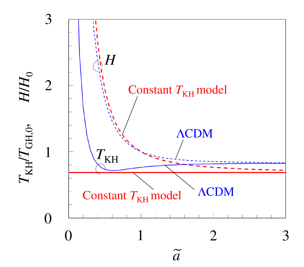
Figure 1 shows evolutions of and for the constant model and the CDM model. The normalized for both models is given by Eq. (82). The horizontal axis represents the normalized scale factor . Similar forms of evolution have been examined in Refs. Koma19 ; Koma20 . As shown in Fig. 1, the normalized for both models decreases with and gradually approaches a positive value, corresponding to that for each de Sitter universe. In contrast, the normalized for the constant model is constant during the evolution of the universe even though the Hubble parameter varies with . The constant value is given by , from Eq. (82). In this way, the normalized for the constant model is different from that for the CDM model. The difference should affect thermodynamic quantities, such as , as examined later. Of course, finally, the normalized approaches for each de Sitter universe.
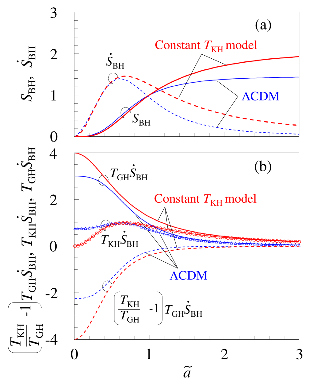
Figure 2 shows the evolution of thermodynamic quantities for the constant model and the CDM model. The normalized and are given by Eqs. (78) and (80), respectively, and are plotted in Fig. 2(a). As shown in Fig. 2(a), the normalized for both models increases with and gradually approaches each positive value. The normalized for both models is positive because the normalized increases with . That is, the second law of thermodynamics, , is satisfied on the horizon. Also, the normalized for both models initially increases and then decreases with , and gradually approaches zero, corresponding to de Sitter universes. In this way, the evolution of and for the constant model is not very different from that for the CDM model. We note that similar discussions of the entropic parameters examined above are given in the previous work Koma19 .
Figure 2(b) shows evolutions of three terms included in the modified thermodynamic relation for constant . From Eq. (49), the relationship between the three terms can be summarized as
| (69) |
First, we observe the evolution of the right-hand side of Eq. (69), namely . The normalized for both models is given by Eq. (83). As shown in Fig. 2(b), initially, the normalized for the constant model is different from that for the CDM model. This is because the normalized for both models is different from each other, especially in the initial stage, as examined in Fig. 1. Note that for the constant model is equivalent to , because of given by Eq. (60).
Next, we observe evolutions of the first and second terms on the left-hand side of Eq. (69). The first and second terms, namely the and terms, are equivalent to and , respectively. The two normalized thermodynamic quantities for both models are given by Eqs. (86) and (87) and are plotted in Fig. 2(b). As shown in Fig. 2(b), initially, the evolutions of the two normalized terms for the constant model are quantitatively different from those for the CDM model. The normalized is positive, whereas the normalized is negative. Specifically, the two initial values for the constant model are and , respectively, whereas the two initial values for the CDM model are and , respectively, as examined in Appendix B. The sum of the normalized first and second terms is equivalent to the normalized , because this relation is given by Eq. (69). (The initial value depends on , where and are set for the CDM and constant models, respectively, as examined in Appendix B.)
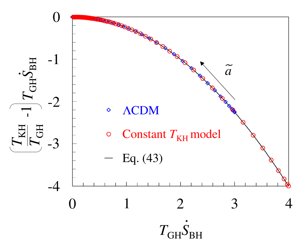
As discussed previously, Eqs. (42) and (43) indicate that the magnitude of the second term (the term) is proportional to the square of the first term (the term). To confirm this, we examine the relationship between the two normalized terms for the constant model and the CDM model, as shown in Fig. 3. The arrow indicates the direction in which the normalized scale factor increases from to . In this figure, the initial coordinate values corresponding to for the constant model and the CDM model are and , respectively. As increases, the normalized plots gradually approach the origin of the coordinates, , corresponding to those for de Sitter universes. We can confirm that all the normalized plots for both models show a quadratic curve. The quadratic curve is described by Eq. (43), which is derived without using specific cosmological models. The relationship between the two terms is universal when the modified thermodynamic relation for constant is satisfied.
In this section, we observed typical evolutions of the thermodynamic quantities in the modified thermodynamic relation using the CDM model and the constant model. The constant model is simply one viable scenario with a constant horizon temperature Koma19 . However, the results for the constant model will contribute to the study of thermodynamics and statistical physics on dynamic horizons because the horizon temperature is constant. For example, a constant universe always satisfies the holographic equipartition law of energy. Therefore, the emergence of cosmic space based on the law Padma2010 ; Verlinde1 ; HDE ; Padmanabhan2004 ; ShuGong2011 ; Koma14 ; Koma15 ; Koma16 ; Koma17 ; Koma19 ; Koma20 ; Padma2012AB ; Cai2012 ; Hashemi ; Moradpour ; Wang ; Koma10 ; Koma11 ; Koma12 ; Koma18 ; Krishna20172019 ; Mathew2022 ; Chen2022 ; Luciano ; Mathew2023 ; Mathew2023b ; Pad2017 ; Tu2018 ; Tu2019 ; Chen2024 , which can lead to cosmological equations, should be discussed from a different viewpoint, using the modified thermodynamic relation. Of course, in general, the modified thermodynamic relation is given by Eq. (29) and the cosmological equations are given by Eqs. (1)–(3). In this case, we should examine the cosmological constant problem, by applying the second law of thermodynamics to the equations and extending a method used in previous works Koma11 ; Koma12 . These tasks are left for future research.
The modified thermodynamic relation examined in this paper should help to understand the properties of various cosmological models from a thermodynamic viewpoint. The present study should provide new insights into the discussion of thermodynamic cosmological scenarios.
VI Conclusions
We examined the holographic-like thermodynamic relation between a cosmological horizon and the bulk by applying a general formulation for cosmological equations to the first law of thermodynamics. For the general formulation, both an effective pressure for dissipative universes and an extra driving term for non-dissipative universes are phenomenologically assumed in a flat FLRW universe. We derived the modified thermodynamic relation that includes both and an additional time-derivative term , by applying the general formulation to the first law. When is constant, the modified thermodynamic relation reduces to the formulation of the first law in standard cosmology.
Next, we examined the modified thermodynamic relation for constant , with considered. The left-hand side of the relation describes thermodynamic quantities in the bulk and can be interpreted as consisting of contributions from two terms, namely the and terms. It is found that the term is equivalent to , and the term is equivalent to . The former equivalence can lead to the Friedmann equation, while the latter can lead to the acceleration equation by coupling with the derived Friedmann equation. The magnitude of the term is proportional to the square of the term. In addition, we applied the equipartition law of energy on the horizon to the term, namely the right-hand side of the modified thermodynamic relation. Consequently, when is constant, the modified thermodynamic relation reduces to . This thermodynamic relation is considered to be a kind of extended holographic-like connection.
Finally, we observed typical evolutions of the thermodynamic quantities in the modified thermodynamic relation for constant using CDM models and a constant model. Initially, thermodynamic quantities which include for both models are different although the evolution of the Hubble parameter is similar between the two models. These thermodynamic quantities for both models gradually approach constant values corresponding to those for de Sitter universes.
The assumptions used in this paper have not yet been established but are considered to be viable scenarios. The modified thermodynamic relation for a constant universe implies that the free-energy difference on the horizon plays important roles. The present study should contribute to a better understanding of the thermodynamic relation between the cosmological horizon and the bulk and should provide new insights into thermodynamics and cosmological equations.
Appendix A Holographic-like connection
Padmanabhan Pad2017 derived an energy-balance relation , which is essentially equivalent to a holographic-like connection, . This appendix briefly reviews the holographic-like connection based on previous works Koma18 ; Koma20 .
We first calculate from the Friedmann equation in standard cosmology Koma18 ; Koma20 . Substituting into Eq. (1), the Friedmann equation is written as
| (70) |
Substituting Eqs. (70) and (24) into Eq. (22) yields
| (71) |
Next, we calculate from the equipartition law of energy on the horizon, using and , where is the Gibbons–Hawking temperature. Substituting Eqs. (13) and (16) into Eq. (56) yields
| (72) |
From Eqs. (71) and (72), we have the relation
| (73) |
This consistency is the holographic-like connection in standard cosmology Koma18 ; Koma20 . (Note that only the magnitudes of and are considered.) The holographic-like connection has not yet been established. In fact, the energy in the equipartition law has been discussed from different viewpoints, e.g., in the works of Verlinde Verlinde1 and Padmanabhan Padma2010 ; Padma2012AB , as described in Ref. Koma20 .
In the above derivation, standard cosmology and the equipartition law of energy on the horizon are assumed. In addition, is used for , instead of a dynamical Kodama–Hayward temperature . In this sense, the holographic-like connection should correspond to a thermodynamic relation for de Sitter universes whose Hubble volume is constant. In the present paper, we extend this connection to the thermodynamic relation in universes whose Hubble volume varies with time.
Appendix B Thermodynamic quantities for a power-law model
In this appendix, we calculate the thermodynamic quantities for a power-law model Koma11 ; Koma16 ; Koma19 . In fact, a constant model is obtained from the power-law model by setting and . The thermodynamic quantities calculate here are used for the constant model. (CDM models are descried in Sec. V.)
First, we again focus on the power-law model. From Eq. (62), the cosmological equation is given by
| (74) |
where and are considered Koma19 . From Eq. (63), the solution of Eq. (74) for is written as Koma14 ; Koma20
| (75) |
where and are given by
| (76) |
We now calculate several thermodynamic quantities for the power-law model, according to Ref. Koma19 . From Eq. (13), the normalized is written as
| (77) |
Substituting Eq. (75) into Eq. (77) yields
| (78) |
In addition, we calculate for the power-law model. Substituting Eq. (74) into given by Eq. (15) and applying Eq. (75) yields Koma19
| (79) |
Using Eq. (79) and , the normalized is written as Koma19
| (80) |
This equation indicates that is satisfied when and are considered. The second law of thermodynamics and the maximization of the entropy have been examined in previous works Koma14 ; Koma19 .
Next, we calculate the normalized Kodama–Hayward temperature for the power-law model. From Eq. (17), the normalized Kodama–Hayward temperature is written as Koma19 ; Koma20
| (81) |
where is used. From Eq. (74), the power-law model satisfies , because and the non-negative driving terms are considered. Therefore, the normalized is non-negative in an expanding universe. Substituting Eq. (74) into Eq. (81), substituting Eq. (75) into the resulting equation, and performing several calculations yields Koma19
| (82) |
When and are considered, this equation reduces to a constant value given by . That is, the power-law model for and corresponds to a constant model Koma19 .
Finally, we calculate the first and second terms on the left-hand side of Eq. (69), namely the and terms, equivalent to and , respectively. Substituting Eq. (74) into Eq. (40) and applying Eq. (75) yields
| (84) |
Similarly, substituting Eq. (74) into Eq. (41) and applying Eq. (75) yields
| (85) |
The same equation can be obtained from Eqs. (42) and (84). For the normalization, dividing Eq. (84) by yields the normalized first term:
| (86) |
To calculate the initial value, we set , although inflation of the early universe is not discussed. When , the normalized first term reduces to and, therefore, the normalized initial value for and is and , respectively. In this way, the normalized initial value depends on . Similarly, from Eq. (85), the normalized second term is given by
| (87) |
When , the normalized second term for and is and , respectively.
Note that the numerical coefficients in Eqs. (86) and (87) are different from those in Eqs. (84) and (85), respectively, because Eqs. (86) and (87) have been normalized by , which includes a coefficient of .
Appendix C Euclidean action and a general ‘action–entropy relation’
The equipartition law of energy on the horizon used in Sec. IV.2 has not yet been established but is considered to be a viable scenario. In this appendix, we discuss the equipartition law from a different viewpoint. In fact, given by Eq. (54), which is based on the equipartition law, can be obtained from Euclidean action and a general ‘action–entropy relation’. This derivation is examined.
We first introduce a general relationship between an action and an entropy , according to the work of de Broglie Broglie . The general ‘action–entropy relation’ can be written as Broglie
| (89) |
where the Planck constant has been replaced by the reduced Planck constant ActionEntropy . We assume that Eq. (89) is satisfied on a cosmological horizon.
Next, according to the work of Gibbons and Hawking GibbonsHawking1977Action , we introduce the relationship between the Helmholtz free energy and Euclidean action of black holes, which is approximately written as York1988 ; Whiting1990 ; Wei2022
| (90) |
where the Wick rotation () has been used and represents the inverse temperature given by . In fact, Eq. (90) can be applied to the cosmological horizon such as the Hubble horizon, as examined in the work of Arias et al. Arias2020 . Therefore, we assume that Eq. (90) can be applied to the Hubble horizon.
Accepting these assumptions, setting , and substituting Eq. (90) into Eq. (89) yields
| (91) |
where , , and have been replaced by , , and , respectively. is not used. Consequently, the free energy on the horizon is given by
| (92) |
This equation is consistent with Eq. (56). Substituting Eq. (92) into the definition of the free energy, , yields
| (93) |
which is consistent with Eq. (54). In addition, from , we can obtain , corresponding to Eq. (52), when given by Eq. (53) is applied. In this way, the equipartition law is likely consistent with the free energy calculated from Euclidean action and the general ‘action–entropy relation’. This consistency may be satisfied not only in de Sitter universes but also in a constant universe discussed in the present study. The above result implies that the equipartition law is a viable scenario. Several assumptions used here have not yet been established and further studies are needed.
References
- (1) S. Perlmutter et al., Nature (London) 391, 51 (1998); A. G. Riess et al., Astron. J. 116, 1009 (1998).
- (2) O. Farooq, F. R. Madiyar, S. Crandall, B. Ratra, Astrophys. J. 835, 26 (2017).
- (3) N. Aghanim et al., Astron. Astrophys. 641, A6 (2020).
- (4) K. Freese, F. C. Adams, J. A. Frieman, E. Mottola, Nucl. Phys. B287, 797 (1987); J. M. Overduin, F. I. Cooperstock, Phys. Rev. D 58, 043506 (1998).
- (5) S. Nojiri, S. D. Odintsov, Phys. Lett. B 639, 144 (2006); J. Solà, J. Phys. Conf. Ser. 453, 012015 (2013).
- (6) S. Basilakos, M. Plionis, J. Solà, Phys. Rev. D 80, 083511 (2009); M. Rezaei, J. Solà Peracaula, M. Malekjani, Mon. Not. R. Astron. Soc. 509, 2593 (2022).
- (7) A. Gómez-Valent, J. Solà, S. Basilakos, J. Cosmol. Astropart. Phys. 01 (2015) 004; M. Rezaei, M. Malekjani, J. Solà Peracaula, Phys. Rev. D 100, 023539 (2019).
- (8) I. Prigogine, J. Geheniau, E. Gunzig, P. Nardone, Proc. Natl. Acad. Sci. U.S.A. 85, 7428 (1988).
- (9) M. O. Calvão, J. A. S. Lima, I. Waga, Phys. Lett. A 162, 223 (1992); J. A. S. Lima, A. S. M. Germano, L. R. W. Abramo, Phys. Rev. D 53, 4287 (1996).
- (10) T. Harko, Phys. Rev. D 90, 044067 (2014); S. R. G. Trevisani, J. A. S. Lima, Eur. Phys. J. C 83, 244 (2023).
- (11) M. P. Freaza, R. S. de Souza, I. Waga, Phys. Rev. D 66, 103502 (2002); V. H. Cárdenas, M. Cruz, S. Lepe, S. Nojiri, S. D. Odintsov, Rev. D 101, 083530 (2020).
- (12) J. D. Barrow, Phys. Lett. B 180, 335 (1986); J. A. S. Lima, R. Portugal, I. Waga, Phys. Rev. D 37, 2755 (1988).
- (13) I. Brevik, S. D. Odintsov, Phys. Rev. D 65, 067302 (2002); S. D. Odintsov, D. Sáez-Chillón Gómez, G. S. Sharov, Phys. Rev. D 101, 044010 (2020).
- (14) J. Yang, Rui-Hui Lin, Xiang-Hua Zhai, Eur. Phys. J. C 82, 1039 (2022).
- (15) D. A. Easson, P. H. Frampton, G. F. Smoot, Phys. Lett. B 696, 273 (2011); Y. F. Cai, E. N. Saridakis, Phys. Lett. B 697, 280 (2011).
- (16) S. Basilakos, D. Polarski, J. Solà, Phys. Rev. D 86, 043010 (2012); S. Basilakos, J. Solà, Phys. Rev. D 90, 023008 (2014).
- (17) N. Komatsu, S. Kimura, Phys. Rev. D 87, 043531 (2013), Phys. Rev. D 88, 083534 (2013).
- (18) N. Komatsu, S. Kimura, Phys. Rev. D 89, 123501 (2014).
- (19) N. Komatsu, S. Kimura, Phys. Rev. D 90, 123516 (2014).
- (20) N. Komatsu, S. Kimura, Phys. Rev. D 92, 043507 (2015).
- (21) N. Komatsu, S. Kimura, Phys. Rev. D 93, 043530 (2016).
- (22) E. M. C. Abreu, J. A. Neto, Phys. Lett. B 824, 136803 (2022).
- (23) H. Gohar, V. Salzano, Phys. Rev. D 109, 084075 (2024).
- (24) R. G. Cai, S. P. Kim, J. High Energy Phys. 02 (2005) 050.
- (25) R. G. Cai, L. M. Cao, N. Ohta, Phys. Rev. D 81, 061501(R) (2010).
- (26) R. G. Cai, L. M. Cao, Phys. Rev. D 75, 064008 (2007).
- (27) R. G. Cai, L. M. Cao, Y. P. Hu, Classical Quantum Gravity 26, 155018 (2009); S. Mitra, S. Saha, S. Chakraborty, Phys. Lett. B 734, 173 (2014).
- (28) A. Sheykhi, Phys. Rev. D 81, 104011 (2010); S. Mitra, S. Saha, S. Chakraborty, Mod. Phys. Lett. A 30, 1550058 (2015).
- (29) K. Karami, A. Abdolmaleki, Z. Safari, S. Ghaffari, J. High Energy Phys. 08 (2011) 150. A. Sheykhi, S. H. Hendi, Phys. Rev. D 84, 044023 (2011).
- (30) P. S. Ens, A. F. Santos, Phys. Lett. B 835,137562 (2022).
- (31) A. Sheykhi, Phys. Rev. D 103, 123503 (2021); Phys. Rev. D 107, 023505 (2023); A. Sheykhi, Phys. Lett. B 785, 118 (2018); 850, 138495 (2024).
- (32) S. Nojiri, S. D. Odintsov, T. Paul, Phys. Lett. B 835, 137553 (2022).
- (33) M. Akbar, R. G. Cai, Phys. Rev. D 75 084003 (2007).
- (34) M. Akbar, R. G. Cai, Phys. Lett. B 648, 243 (2007).
- (35) R. G. Cai, L. M. Cao, Y. P. Hu, J. High Energy Phys. 08 (2008) 090.
- (36) L. M. Sánchez, H. Quevedo, Phys. Lett. B 839, 137778 (2023).
- (37) S. Nojiri, S. D. Odintsov, T. Paul, S. SenGupta, Phys. Rev. D 109, 043532 (2024).
- (38) S. D. Odintsov, D’Onofrio, T. Paul, Physics of the Dark Universe 42 (2023) 101277.
- (39) S. D. Odintsov, T. Paul, S. SenGupta, Phys. Rev. D 109, 103515 (2024).
- (40) S. D. Odintsov, S. D’Onofrio, T. Paul, Phys. Rev. D 110, 043539 (2024).
- (41) A. Khodam-Mohammadi, M. Monshizadeh, Phys. Lett. B 843,138066 (2023).
- (42) R. Easther, D. Lowe, Phys. Rev. Lett. 82, 4967 (1999); C. A. Egan, C. H. Lineweaver, Astrophys. J. 710, 1825 (2010).
- (43) J. P. Mimoso, D. Pavón, Phys. Rev. D 87, 047302 (2013).
- (44) K. Bamba, A. Jawad, S. Rafique, H. Moradpour, Eur. Phys. J. C 78, 986 (2018); M. Gonzalez-Espinoza, D. Pavón, Mon. Not. R. Astron. Soc. 484, 2924 (2019).
- (45) L. Dyson, M. Kleban, L. Susskind, J. High Energy Phys. 10 (2002) 011.
- (46) S. Pan, W. Yang, C. Singha, E. N. Saridakis, Phys. Rev. D 100, 083539 (2019).
- (47) E. N. Saridakis, S. Basilakos, Eur. Phys. J. C 81, 644 (2021).
- (48) M. Sharif, M. Zeeshan Gul, N. Fatima, Eur. Phys. J. C 84,1065 (2024).
- (49) T. Padmanabhan, Mod. Phys. Lett. A 25, 1129 (2010).
- (50) E. Verlinde, J. High Energy Phys. 04 (2011) 029.
- (51) A. Sayahian Jahromi, S. A. Moosavi, H. Moradpour, J. P. Morais Graça, I. P. Lobo, I. G. Salako, A. Jawad, Phys. Lett. B 780, 21 (2018).
- (52) T. Padmanabhan, Classical Quantum Gravity 21, 4485 (2004).
- (53) Fu-Wen Shu, Y. Gong, Int. J. Mod. Phys. D 20, 553 (2011).
- (54) N. Komatsu, Phys. Rev. D 100, 123545 (2019).
- (55) N. Komatsu, Phys. Rev. D 102, 063512 (2020).
- (56) N. Komatsu, Phys. Rev. D 103, 023534 (2021).
- (57) N. Komatsu, Phys. Rev. D 105, 043534 (2022).
- (58) N. Komatsu, Phys. Rev. D 108, 083515 (2023).
- (59) N. Komatsu, Phys. Rev. D 109, 023505 (2024).
- (60) T. Padmanabhan, arXiv:1206.4916 [hep-th]; Res. Astron. Astrophys. 12, 891 (2012).
- (61) R. G. Cai, J. High Energy Phys. 1211 (2012) 016; S. Chakraborty, T. Padmanabhan, Phys. Rev. D 92, 104011 (2015).
- (62) M. Hashemi, S. Jalalzadeh, S. V. Farahani, Gen. Relativ. Gravit. 47, 53 (2015).
- (63) H. Moradpour, Int. J. Theor. Phys. 55, 4176 (2016).
- (64) J. Wang, Gen. Relativ. Gravit. 49, 145 (2017).
- (65) N. Komatsu, Eur. Phys. J. C 77, 229 (2017).
- (66) N. Komatsu, Phys. Rev. D 96, 103507 (2017).
- (67) N. Komatsu, Phys. Rev. D 99, 043523 (2019).
- (68) N. Komatsu, Eur. Phys. J. C 83, 690 (2023).
- (69) P. B. Krishna, T. K. Mathew, Phys. Rev. D 96, 063513 (2017); Phys. Rev. D 99, 023535 (2019).
- (70) P. B. Krishna, V. T. H. Basari, T. K. Mathew, Gen. Relativ. Gravitat. 54, 58 (2022).
- (71) G. R. Chen, Eur. Phys. J. C 82, 532 (2022).
- (72) G. G. Luciano, Phys. Lett. B 838, 137721 (2023).
- (73) M. Muhsinath, V. T. H. Basari, T. K. Mathew, Gen. Relativ. Gravitat. 55, 43 (2023).
- (74) M. T. Manoharan, N. Shaji, T. K. Mathew, Eur. Phys. J. C 83, 19 (2023).
- (75) T. Padmanabhan, Comptes Rendus Physique 18, 275 (2017).
- (76) Fei-Quan Tu, Yi-Xin Chen, Bin Sun, You-Chang Yang, Phys. Lett. B 784, 411 (2018).
- (77) Fei-Quan Tu, Yi-Xin Chen, Qi-Hong Huang, Entropy 21, 167 (2019).
- (78) J. Chen, G. Chen, Eur. Phys. J. C 84, 1178 (2024).
- (79) S. W. Hawking, Phys. Rev. Lett. 26, 1344 (1971); Nature (London) 248, 30 (1974); Commun. Math. Phys. 43, 199 (1975); Phys. Rev. D 13, 191 (1976); J. D. Bekenstein, Phys. Rev. D 7, 2333 (1973); Phys. Rev. D 9, 3292 (1974); Phys. Rev. D 12, 3077 (1975).
- (80) G. ’t Hooft, Conf. Proc. C 930308, 284 (1993) [arXiv:gr-qc/9310026]; L. Susskind, J. Math. Phys. 36, 6377 (1995); R. Bousso, Rev. Mod. Phys. 74, 825 (2002).
- (81) G. W. Gibbons, S. W. Hawking, Phys. Rev. D 15, 2738 (1977).
- (82) S. A. Hayward, Classical Quantum Gravity 15, 3147, (1998).
- (83) S. A. Hayward, R. D. Criscienzo, M. Nadalini, L. Vanzo, S. Zerbini, Classical Quantum Gravity 26, 062001 (2009).
- (84) B. Ryden, Introduction to Cosmology (Addison-Wesley, Reading, MA, 2002).
- (85) J. D. Barrow, T. Clifton, Phys. Rev. D 73, 103520 (2006).
- (86) B. Wang, Y. Gong, E. Abdalla, Phys. Lett. B 624, 141 (2005).
- (87) J. A. S. Lima, S. Basilakos, J. Solà, Mon. Not. R. Astron. Soc. 431, 923 (2013).
- (88) S. Das, S. Shankaranarayanan, S. Sur, Phys. Rev. D 77, 064013 (2008).
- (89) N. Radicella, D. Pavón, Phys. Lett. B 691, 121 (2010).
- (90) A. Chatterjee, P. Majumdar, Phys. Rev. Lett. 92, 141301 (2004).
- (91) C. Tsallis, L. J. L. Cirto, Eur. Phys. J. C 73, 2487 (2013).
- (92) T. S. Biró, V. G. Czinner, Phys. Lett. B 726, 861 (2013).
- (93) J. D. Barrow, Phys. Lett. B 808, 135643 (2020).
- (94) S. Nojiri, S. D. Odintsov, V. Faraoni, Phys. Rev. D 105, 044042 (2022).
- (95) I. Çimdiker, M. P. Da̧browski, H. Gohar, Eur. Phys. J. C 83, 169 (2023).
- (96) H. B. Callen, Thermodynamics and an introduction to thermostatistics, 2nd ed. (Wiley, New York, 1985).
- (97) G. W. Gibbons, S. W. Hawking, Phys. Rev. D 15, 2752 (1977).
- (98) J. W. York, Phys. Rev. D 33, 2092 (1986).
- (99) B. F. Whiting, J. W. York, Phys. Rev. Lett. 61, 1336 (1988).
- (100) B. F. Whiting, Class. Quantum Grav. 7, 15 (1990).
- (101) Shao-Wen Wei, Yu-Xiao Liu, R. B. Mann, Phys. Rev. Lett. 129, 191101 (2022).
- (102) L. de Broglie, Thermodynamics of Isolated Particle (Hidden Thermodynamics of Particles), (Gauthier-Villars, Paris, 1964).
- (103) D. Acosta, P. F. de Cordoba, J. M. Isidro, J. L. G. Santander, Int. J. Geom. Meth. Mod. Phys. 10, 1350007 (2013).
- (104) S. Ryu, T. Takayanagi, Phys. Rev. Lett. 96, 181602 (2006); J. High Energy Phys. 08 (2006) 045.
- (105) C. Arias, F. Diaz, P. Sundell, Classical Quantum Gravity 37, 015009 (2020).
- (106) D. D. Blanco, H. Casini, Ling-Yan Hung, R. C. Myers, J. High Energy Phys. 08 (2013) 060; D. L. Jaeris, A. Lewkowycz, J. Maldacena, S. J. Suh, J. High Energy Phys. 06 (2016) 004.