Holographic description of entanglement entropy of free CFT on torus

The holographic principle of gravity proposes that the degrees of freedom of $d+1$-dimensional gravity is that of $d$-dimensional theory without gravity. This perspective is originated from the Beckenstein-Hawking formula that the black hole entropy is the area of its event horizon. The AdS/CFT correspondence Maldacena:1997re ; Gubser:1998bc ; Witten:1998qj provides a toy model to investigate the holographic property of gravity. The Ryu-Takayanagi conjecture Ryu:2006bv ; Ryu:2006ef is a generalization of the Beckenstein-Hawking formula. It is believed to give a gravity dual of the entanglement entropy(EE) of the strongly coupled holographic CFTs in the semi-classical limit. Let $\rho_{A}$ denote the reduced density matrix of a space-like region $A$ in CFT, then the EE $S_{A}$ of a region $A$ is defined as

$\displaystyle S_{A}=-\mathrm{Tr}_{A}\left(\rho_{A}\log\rho_{A}\right).$

(1)

For the semi-classical limit CFT, the Ryu-Takayanagi conjecture provides the EE of a region $A$ as

$\displaystyle S_{A}=\frac{\mathrm{Area\ of\ }\gamma_{A}}{4G},$

(2)

where $G$ is the gravitational constant and $\gamma_{A}$ is the global minimal surface in the dual bulk spacetime, that is homologous to the sub-system on the AdS boundary Headrick:2007km . This conjecture has played a fundamental role in studying this issue and shed light on the relationship between the AdS/CFT correspondence and the information theory. It also brings many information-theoretical analyses Swingle:2009bg ; Pastawski:2015qua ; Lashkari:2013koa ; Dong:2016eik of the AdS/CFT correspondence. Thus, it is perhaps the most fundamental key to grasping the AdS/CFT correspondence.

We will focus on the EE of one interval for free massless fermion or boson on the torus Azeyanagi:2007bj ; Datta:2013hba . We will see that the common terms in them can be described as the sum of the signed area of the extremal surfaces in the BTZ spacetime. Although a free CFT does not have the gravity dual, it is interesting to describe the EE of free CFTs in an holographic way, because it presents a geometrical point of view for the EE of free CFT and it allows us to compare the EEs between holographic CFTs and free CFTs. In addition, we will see that the configuration of the extremal surfaces and their signs has a geometrical consistency between the CFT side and the gravity side. Surprisingly, the resulting EE is smaller than the holographic EE given by the Ryu-Takayanagi formula and the corresponding bunch of the extremal surfaces has preferable holographic properties.

The construction of this paper is as follows. In section 2, we will review the replica trick and discuss the geometrical consistency between the replica manifold of the CFT side and the gravity side. In section 3, we will see the extremal surfaces in the BTZ spacetime. In section 4, we will point out that the EE of one interval for free massless fermion on the torus is described by the sum of signed area of all the extremal surfaces that extend from the edge of the interval on the AdS boundary. Finally, section 5 is the conclusion.

We will investigate the geometry of the replica manifold and find that it has the conical singularities at the edge of a region. Eq.(1) can be rewritten by the replica trick Calabrese:2004eu ; Calabrese:2009qy as

$\displaystyle S_{A}=\lim_{n\to 1}S^{(n)}_{A},\ \ \ S^{(n)}_{A}:=\frac{1}{1-n}\log\mathrm{tr}_{A}\left(\rho_{A}^{\ n}\right).$

(3)

For convenience, we will consider the Renyi entropy $S^{(n)}_{A}$ in the following discussion. Let $Z$ be the partition function of a CFT on a manifold $\mathcal{B}$, and $Z_{A}^{(n)}$ be partition function of the same CFT on the replica manifold $\mathcal{B}_{A}^{(n)}$. Since $Z_{A}^{(n)}$ satisfies $\mathrm{tr}_{A}\left(\rho_{A}^{\ n}\right)=Z_{A}^{(n)}/Z^{n}$, the Renyi entropy $S^{(n)}_{A}$ is written by the partition functions as

$\displaystyle S^{(n)}_{A}=\frac{1}{1-n}\left(\log Z_{A}^{(n)}-n\log Z\right).$

(4)

For example, consider $\mathcal{B}=\mathbb{C}\cup\{\infty\}$ and $A=[u,v]$. Instead of performing the path integral on the corresponding replica manifold $\mathcal{B}_{A}^{(n)}$, we can evaluate the Renyi entropy of $A$ as the following 2-point correlation function.

$\displaystyle S^{(n)}_{A}=\frac{1}{1-n}\log\langle\mathcal{T}_{n}(u)\mathcal{\tilde{T}}_{n}(v)\rangle_{\mathcal{B}}=\frac{c(1+n)}{6n}\log\frac{|u-v|}{\epsilon}+\mathrm{cnst}.$

(5)

where $\mathcal{T}_{n}$ and $\mathcal{\tilde{T}}_{n}$ are the primary twist operators with the conformal weight $h=c(n^{2}-1)/24n$.

To investigate the geometry of the replica manifold $\mathcal{B}_{A}^{(n)}$ with $\mathcal{B}=\mathbb{C}\cup\{\infty\}$ and $A=[u,v]$, consider the scale transformation of the Renyi entropy. For a moment, we will abbreviated the lower indices $A$ and specify the quantities defined on $\mathcal{B}^{(n)}$ by the upper index $(n)$. Applying the Ward-Takahashi identity for the scale transformation to eq.(4), we obtain

	$\displaystyle\ell\frac{\partial}{\partial\ell}S^{(n)}$	$\displaystyle=\frac{2}{1-n}\left(\int_{\mathcal{B}^{(n)}}d^{2}x\,g^{(n)}_{\mu\nu}\frac{\delta}{\delta g^{(n)}_{\mu\nu}}\log Z^{(n)}-n\,\int_{\mathcal{B}}d^{2}x\,g_{\mu\nu}\frac{\delta}{\delta g_{\mu\nu}}\log Z\right)$
		$\displaystyle=\frac{c}{24\pi(1-n)}\left(\int_{\mathcal{B}^{(n)}}d^{2}x\,\sqrt{\left|g^{(n)}\right|}R^{(n)}-n\,\int_{\mathcal{B}}d^{2}x\,\sqrt{\left|g\right|}R\right).$		(6)

where $\ell$ is a scale of the system, and $g_{\mu\nu},g$ and $R$ are the metric, the determinant of the metric and the Ricci scalar, respectively. Compered with eq.(5), the replica manifold $\mathcal{B}_{A}^{(n)}$ should be singular at $\partial A=\{u,v\}$ and we can consider the Ricci scalar as $R^{(n)}=-2\pi(n-1/n)\delta(t)(\delta(x-u)+\delta(x-v))$. Thus, there exists the conical deficit with angle $\Delta\phi=\pi(n-1/n)$ on the replica manifold at $\partial A$.

We can also confirm that there exists conical singularity with angle $\Delta\phi=\pi(n-1/n)$ at $\partial A$ considering a CFT on $\mathbb{C}/\mathbb{Z}_{N}$ Nishioka:2006gr , where $\mathbb{Z}_{N}=\mathbb{Z}/N$ and $N$ denotes an positive integer. Consider a free massless scalar field on $\mathbb{C}/\mathbb{Z}_{N}$ with the central charge $c$. Let $N=1/n$ and the sub-system $A=[0,\infty)$, then the partition function $Z_{A}^{(1/N)}$ is

	$\displaystyle\log Z_{A}^{(1/N)}$	$\displaystyle=\frac{1}{N}\log Z+\frac{c}{N}\sum_{j=1}^{N-1}\int_{\mathbb{C}}dzd\bar{z}\,\delta(z-e^{\frac{2\pi i}{N}j}z)\delta(\bar{z}-e^{-\frac{2\pi i}{N}j}\bar{z})\,\log\frac{\Lambda}{\epsilon}$
		$\displaystyle=\frac{1}{N}\log Z+\frac{c(N^{2}-1)}{12N}\int_{\mathbb{C}/\mathbb{Z}_{N}}d^{2}x\,\delta(t)\delta(x)\,\log\frac{\Lambda}{\epsilon}$		(7)

where $\Lambda$ and $\epsilon$ are the IR and UV cutoff lengths, respectively. Compared with eq.(2), we can understand that there exists conical singularity with angle $\Delta\phi=\pi(n-1/n)$ at a single edge of the interval $A$.

Focus on the gravity dual of the above replica manifold $\mathcal{B}_{A}^{(n)}$. Consider the $2+1$-dimensional replica bulk manifold $\mathcal{M}_{A}^{(n)}$ of which boundary is the $1+1$ dimensional replica manifold $\mathcal{B}^{(n)}_{A}$ in the sense that $\partial\mathcal{M}_{A}^{(n)}=\mathcal{B}_{A}^{(n)}$. Since $\mathcal{B}_{A}^{(n)}$ has the conical singularities as discussed above, the replica bulk manifold $\mathcal{M}_{A}^{(n)}$ should have the canical singularities in the geometricary consistent manner. As the cosmic string with string tension $(n^{2}-1)/8nG$ that makes the singularities with deficit angle $\pi(n-1/n)$ around it for $n\sim 1$, it is natural to consider that the replica bulk manifold $\mathcal{M}_{A}^{(n)}$ contains the cosmic string with string tension $(n^{2}-1)/8nG$ Dong:2016fnf . This seems the unique way of constructing the replica bulk manifold $\mathcal{M}_{A}^{(n)}$ consistently about the deficit angles between $\partial\mathcal{M}_{A}^{(n)}$ and $\mathcal{B}_{A}^{(n)}$. However, notice that we can consider for introducing the cosmic string with opposite signed string tension $-(n^{2}-1)/8nG$ and there are more configurations of cosmic strings satisfying this boundary condition than before. Actually, we will see that the Renyi entropy of free CFT with $n\sim 1$ is almost described as many cosmic strings with the both signed string tension satisfying the deficit angle consistency.

The cosmic strings for $n\sim 1$ as mentioned in the previous section behave as $1$-dimensional extremal surfaces. We will see the extremal surfaces in the BTZ spacetime and its areas. The metric of the BTZ spacetime can be described as follows.

$\displaystyle ds^{2}=-\left(\frac{r^{2}}{L^{2}}-M\right)dt^{2}+\left(\frac{r^{2}}{L^{2}}-M\right)^{-1}dr^{2}+r^{2}d\theta^{2},$

(8)

where $M$ is the mass parameter of the black hole and $L$ is the AdS radius, and $t\in[-\infty,\infty]$, $r\in[\sqrt{M}L,\infty]$, $\theta\in[-\pi,\pi]$ and $\theta$-coordinate is periodic. As it is $2+1$-dimensional spacetime, we will derive space-like geodesics that extend from $\partial A:(t,r,\theta)=(0,\infty,\pm\theta_{A})$ into the bulk on the $t=0$ time-slice. Minimizes the following length of a line.

$\displaystyle\mathrm{Length}=\int_{-\theta_{A}}^{\theta_{A}}d\theta\sqrt{\left(\frac{r^{2}}{L^{2}}-M\right)^{-1}\left(\frac{dr}{d\theta}\right)^{2}+r^{2}}.$

(9)

We will introduce the IR cut off scale in this integral later not to diverge for it. From this, a space-like geodesic on the $t=0$ time-slice in BTZ spacetime is described as

$\displaystyle r(\theta)=\frac{\sqrt{M}L\,r_{0}\,\mathrm{sech}\left(\sqrt{M}\,\theta\right)}{\sqrt{ML^{2}-r_{0}^{2}\tanh^{2}\left(\sqrt{M}\,\theta\right)}},$

(10)

where $r_{0}:=r(\theta=0)$. If this geodesic extends from each $(0,\infty,\pm\theta_{A})$, the corresponding values are $r_{0}=\sqrt{M}L\,\mathrm{coth}[\sqrt{M}(m\pi\pm\theta_{A})]$, where $m$ is an integer satisfying $\pi m\pm\theta_{A}>0$. Each length of them are expressed as

$\displaystyle\frac{\mathrm{Length}}{4G}=\frac{L}{2G}\log\left[\frac{2\,r_{\text{max}}}{\sqrt{M}L}\sinh\left(\sqrt{M}\,(m\pi\pm\theta_{A})\right)\right]$

(11)

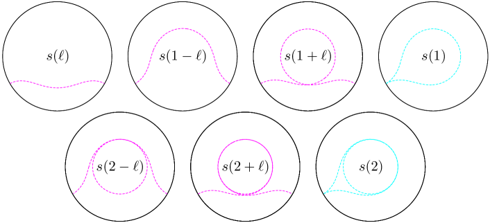
where we integrated from $r=r_{0}$ to $r=r_{\text{max}}$ to avoid the IR divergence, and we assumed $r_{\text{max}}\gg r_{0}$ and ignored the sub-leading terms. For the later discussion, consider the geodesics extend from only $(0,\infty,+\theta_{A})$. We can immediately obtain them by replacing $\theta\to\theta+\theta_{A}$ in eq.(10). In this case, $r_{0}=\sqrt{M}L\,\mathrm{coth}[\sqrt{M}m\pi],\ m=1,2,\cdots$. Each length of them are also expressed as (11) substituting $\theta_{A}=0$. Some of them are depicted in figure 1. Notice that $m$ represents the number of times that the corresponding geodesic passes through the opposite side of the black hole against the interval $[-\theta_{A},\theta_{A}]$ on the AdS boundary. The minimal radius of the geodesic $r_{0}$ approaches to the black hole horizon radius $\sqrt{M}L$ taking $m\to\infty$.

The BTZ black hole spacetime is considered as the dual gravity spacetime of $1+1$ dimensional CFT on torus in the AdS/CFT correspondence. Let us consider CFT defined on $\mathrm{S}^{1}$ of which circumference is $C$ with the UV cutoff length $\epsilon$ and the inverse temperature $\beta$. The bulk parameters are translated into the above CFT quantities as follows. The black hole mass and the IR cut off are $\beta/C=1/\sqrt{M}$ and $\epsilon=L/(2\pi r_{\text{max}})$. The Brown-Henneaux formula Brown:1986nw translates $G$ into the central charge $c$ of CFT as $c=3L/(2G)$. The length of an interval is $\ell:=C\theta_{A}/\pi\in[0,C]$. Then, we can describe eq.(11) as follows.

$\displaystyle s(mC\pm\ell):=\frac{c}{3}\log\left[\frac{\beta}{\pi C\epsilon}\sinh\left\{\frac{\pi(mC\pm\ell)}{\beta}\right\}\right].$

(12)

In the next section, we will see that the EE of one interval for the free massless field on a torus is almost described by an appropriate sum of $\pm s(mC\pm\ell)$.

Consider $1+1$-dimensional CFT on the circle of which circumference $C=1$ at the inverse temperature $\beta$. The common term of the EE of an interval $A=[-\ell/2,\ell/2],\,\ell\in(\epsilon,1-\epsilon)]$ on this system in the high-temperature expansion is as follows Azeyanagi:2007bj ; Datta:2013hba .

	$\displaystyle S_{A}$	$\displaystyle=\frac{c}{3}\left\{\log\left[\frac{\beta}{\pi\epsilon}\sinh\left(\frac{\pi\ell}{\beta}\right)\right]+\sum_{m=1}^{\infty}\log\frac{(1-e^{2\pi\ell/\beta}e^{-2\pi m/\beta})(1-e^{-2\pi\ell/\beta}e^{-2\pi m/\beta})}{(1-e^{-2\pi m/\beta})^{2}}\right\}$
		$\displaystyle=\frac{c}{3}\log\left[\frac{\beta}{\pi\epsilon}\sinh\left(\frac{\pi\ell}{\beta}\right)\right]+\frac{c}{3}\sum_{m=1}^{\infty}\log\frac{\sinh\left[\frac{\pi}{\beta}(m-\ell)\right]\sinh\left[\frac{\pi}{\beta}(m+\ell)\right]}{\sinh^{2}\left(\frac{\pi m}{\beta}\right)}$		(13)

This EE is described as the following sum of signed length of extremal surfaces from eq.(12).

$\displaystyle S_{A}=s(\ell)+\sum_{m=1}^{\infty}\left[s(m-\ell)+s(m+\ell)-2s(m)\right]$

(14)

The corresponding extremal surfaces are depicted as fig. 2.

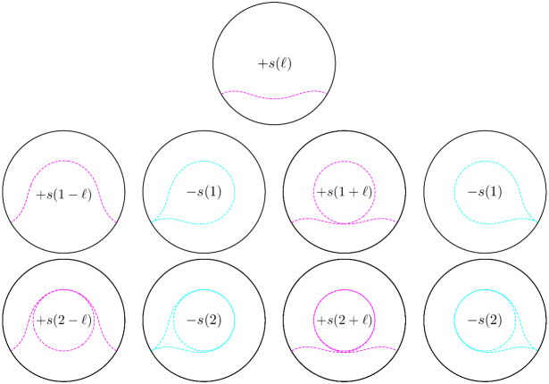
From an algebraic viewpoint, we cannot determine the configurations of each surface. In particular, the surfaces corresponding to $-s(1)$ seem to need not extend from each $\pm\ell/2$. However, from the conical deficit angle consistency as we discussed in section 2, it is natural to describe the surface configuration as depicted in fig. 2.

In what follows, we will comment on this holographic description for free field EE compared with the Ryu-Takayanagi conjecture in the BTZ black hole spacetime. The Ryu-Takayanagi conjecture predicts the corresponding EE as

$\displaystyle S_{A}=\mathrm{min}\left\{s(\ell),\ s(1-\ell)+S_{BH}\right\},$

(15)

where $S_{BH}=c\pi/3\beta$ corresponds with the black hole entropy. We will focus on a few differences between them on geometrical aspects of the configuration of the extremal surfaces corresponding to them. First, the most striking difference between eq.(15) and eq.(14) is the region where the surfaces can sweep. The homologous minimal surface corresponding with the Ryu-Takayanagi conjecture has the entanglement shadow region and the plateaux problem Freivogel:2014lja ; Hubeny:2013gta . Since any homologous minimal surface cannot reach the bulk region near by the black hole horizon, the holographic EE is independent of the property of such a region. On the other hand, since the surfaces corresponding with eq.(14) can sweep all the bulk region outside the black hole horizon, the plateaux problem does not happen. In the same way, since in the higher dimensional Schwarzschild-AdS black hole there are surfaces that can approach the black hole horizon infinitesimally, the plateaux problem may not happen for free CFT as well.

Second, we will see the relation between surfaces of eq.(14) and the black hole horizon. Although eq.(14) seems not to include the black hole horizon explicitly, if $A=1-\delta,\,\epsilon<\delta\ll 1$, eq.(14) becomes

	$\displaystyle S(1-\delta)$	$\displaystyle=\frac{c}{3}\log\left[\frac{\beta}{\pi\epsilon}\sinh\left(\frac{\pi\delta}{\beta}\right)\right]+\frac{c}{3}\lim_{m\to\infty}\log\frac{\sinh\left(\frac{\pi}{\beta}(m+1)\right)}{\sinh\left(\frac{\pi m}{\beta}\right)}+O(\delta)$
		$\displaystyle=\frac{c}{3}\log\left[\frac{\beta}{\pi\epsilon}\sinh\left(\frac{\pi\delta}{\beta}\right)\right]+\frac{c\pi}{3\beta}.$		(16)

Taking $\delta,\epsilon\to 0$, the Araki-Lieb inequality is saturated and the difference of the EEs corresponds to the black hole entropy $S_{BH}$:

$\displaystyle\lim_{\delta,\epsilon\to 0}S(1-\delta)-S(\delta)=\frac{c\pi}{3\beta}=S_{BH}.$

(17)

The black hole horizon emerges as a result of the difference of the surface wrapped $m+1$ times around the black hole and one wrapped $m$ times taking $m$ to the infinity. Both sides of eq.(17) are equivalent as the surfaces not just as the value.

Finally, we should consider that eq.(14) may describe the holographic EE for the holographic CFTs. The EE given by eq.(14) is smaller than that from the Ryu-Takayanagi formula eq.(15). To consider the hamologous condition, pay attention for the topology of the surface configuration in fig. 2. The total winding number of the surfaces for $m\geq 1$ around the black hole is $0$. Thus, when we regard all the surfaces in fig. 2 as a single surface, it is homotopy equivalence to the sub-region $A$ on the AdS boundary. Therefore, eq.(14) may be the true holographic EE.

We provided a holographic description of the entanglement entropy given by eq.(4) as the sum of the signed areas of the extremal surfaces satisfying the deficit angle consistency. It has preferable properties for the HEE in the following reasons. First, it does not have the entanglement shadow region that the Ryu-Takayanagi conjecture has. Second, the resulting holographic EE eq.(14) gives smaller EE than that from the Ryu-Takayanagi conjecture, and the bunch of the surfaces corresponding with eq.(14) is homotopy equivalent to the sub-system on the AdS boundary. Thus, eq.(14) can be a candidate of the holographic EE for the holographic CFT.

References

- (1) J.M. Maldacena, The Large N limit of superconformal field theories and supergravity, Int. J. Theor. Phys. 38 (1999) 1113 [hep-th/9711200].
- (2) S. Gubser, I.R. Klebanov and A.M. Polyakov, Gauge theory correlators from noncritical string theory, Phys. Lett. B 428 (1998) 105 [hep-th/9802109].
- (3) E. Witten, Anti-de Sitter space and holography, Adv. Theor. Math. Phys. 2 (1998) 253 [hep-th/9802150].
- (4) S. Ryu and T. Takayanagi, Holographic derivation of entanglement entropy from AdS/CFT, Phys. Rev. Lett. 96 (2006) 181602 [hep-th/0603001].
- (5) S. Ryu and T. Takayanagi, Aspects of Holographic Entanglement Entropy, JHEP 08 (2006) 045 [hep-th/0605073].
- (6) M. Headrick and T. Takayanagi, A Holographic proof of the strong subadditivity of entanglement entropy, Phys. Rev. D 76 (2007) 106013 [arXiv:0704.3719].
- (7) B. Swingle, Entanglement Renormalization and Holography, Phys. Rev. D 86 (2012) 065007 [arXiv:0905.1317].
- (8) F. Pastawski, B. Yoshida, D. Harlow and J. Preskill, Holographic quantum error-correcting codes: Toy models for the bulk/boundary correspondence, JHEP 06 (2015) 149 [arXiv:1503.06237].
- (9) N. Lashkari, M.B. McDermott and M. Van Raamsdonk, Gravitational dynamics from entanglement ’thermodynamics’, JHEP 04 (2014) 195 [arXiv:1308.3716].
- (10) X. Dong, D. Harlow and A.C. Wall, Reconstruction of Bulk Operators within the Entanglement Wedge in Gauge-Gravity Duality, Phys. Rev. Lett. 117 (2016) 021601 [arXiv:1601.05416].
- (11) T. Azeyanagi, T. Nishioka and T. Takayanagi, Near Extremal Black Hole Entropy as Entanglement Entropy via AdS(2)/CFT(1), Phys. Rev. D 77 (2008) 064005 [arXiv:0710.2956].
- (12) S. Datta and J.R. David, Rényi entropies of free bosons on the torus and holography, JHEP 04 (2014) 081 [arXiv:1311.1218].
- (13) P. Calabrese and J.L. Cardy, Entanglement entropy and quantum field theory, J. Stat. Mech. 0406 (2004) P06002 [hep-th/0405152].
- (14) P. Calabrese and J. Cardy, Entanglement entropy and conformal field theory, J. Phys. A 42 (2009) 504005 [arXiv:0905.4013].
- (15) T. Nishioka and T. Takayanagi, AdS Bubbles, Entropy and Closed String Tachyons, JHEP 01 (2007) 090 [hep-th/0611035].
- (16) X. Dong, The Gravity Dual of Renyi Entropy, Nature Commun. 7 (2016) 12472 [arXiv:1601.06788].
- (17) J. Brown and M. Henneaux, Central Charges in the Canonical Realization of Asymptotic Symmetries: An Example from Three-Dimensional Gravity, Commun. Math. Phys. 104 (1986) 207.
- (18) B. Freivogel, R. Jefferson, L. Kabir, B. Mosk and I.-S. Yang, Casting Shadows on Holographic Reconstruction, Phys. Rev. D 91 (2015) 086013 [arXiv:1412.5175].
- (19) V.E. Hubeny, H. Maxfield, M. Rangamani and E. Tonni, Holographic entanglement plateaux, JHEP 08 (2013) 092 [1306.4004].