Holograhic two-currents model with coupling and its conductivites
Abstract
We implement a holographic gravity model of two gauge fields with a coupling between them, which is dual to a two-currents model. An analytical black brane solution is obtained. In particular, we work out the expressions of conductivities with coupling and find that the expressions of conductivities are directly related to the coupling parameter . It is the main topic of our present work. As an application, we calculate the conductivities by the scheme outlined here and briefly discuss the properties of the conductivities. An interesting property is that as the coupling increases, the dip at low frequency in / becomes deepening and then turns into a hard-gap-like when , which is independent of the doping . Some monotonic behaviors of the conductivities are also discussed.
I Introduction
AdS/CFT (Anti-de-Sitter/Conformal field theory) correspondence, also referring to holography, provides us a way to study the dynamics of certain strongly-coupled condensed matter systems Maldacena:1997re ; Gubser:1998bc ; Witten:1998qj ; Aharony:1999ti . In the so-called bottom-up approaches, we can study some universal properties of the dual system by constructing a simple gravitational model. Along this direction, some interesting holographic models, for example, the holographic superconductor Hartnoll:2008vx , holographic metal insulator phase transition (MIT) Donos:2012js ; Ling:2014saa and (non-) Fermi liquid Liu:2009dm , have been implemented. These studies provide some physical insight into the associated mechanisms of the strongly-coupled systems and the universality class of them.
Recently, the holographic two-currents models are increasingly drawn attention, see Kiritsis:2015hoa ; Bigazzi:2011ak ; Huang:2020iyw ; Iqbal:2010eh ; Baggioli:2015dwa ; Rogatko:2017tae ; Rogatko:2020vtz ; Seo:2016vks and references therein. In these models, a pair of gauge fields and in bulk are introduced111Some holographic models with two gauge fields are also studied in Ling:2015exa ; Ling:2020mwm ; Ling:2017naw ; Ling:2016wyr ; Tarrio:2011de ; Alishahiha:2012qu , in which only one of gauge fields is treated as the real Maxwell field and we only concentrate on its transport properties. In Ling:2015exa , another gauge field is treated as an auxiliary field, which is introduced to obtain an insulating phase with a hard gap. On top of this novel holographic insulator constructed in Ling:2015exa , a holographic superconductor is also built Ling:2017naw . Further, Ling:2020mwm also introduces a coupling between these two gauge fields and studies the superconducting instability. In Ling:2016wyr , another gauge field is introduced to induce metal-insulator phase transition over Gubser-Rocha background Gubser:2009qt in the limit of of zero temperature. While in Tarrio:2011de ; Alishahiha:2012qu , the additional gauge field also plays the role of the auxiliary field to implement charged hyperscaling or Lifshitz black hole background. Therefore, these models are still treated as single current models.. Therefore, we have two independently conserved currents, which relate to different kinds of chemical potentials or charged densities in the dual boundary field theory. The mismatch of the two controllable chemical potentials or charge densities induces the unbalance of numbers. In Kiritsis:2015hoa ; Baggioli:2015dwa ; Huang:2020iyw , the ration of the two chemical potentials is proposed to simulate the effect of doping. In Bigazzi:2011ak , they propose the holographic two-currents model has a counterpart of Mott’s two-currents model Mott:1936v1 ; Mott:1936v2 . The chemical potential mismatch is interpreted as a chemical potential for a “spin” symmetry Bigazzi:2011ak ; Iqbal:2010eh . And then, on top of the two-current model, they construct an unbalanced s-wave superconductor by introducing a charged complex scalar field Bigazzi:2011ak , which is a simple extension of holographic superconductor in Hartnoll:2008vx . Also they study “charge” and “spin” transport Bigazzi:2011ak 222Some related works are also explored, see for example Erdmenger:2011hp ; Dutta:2013osl ; Correa:2019ivh ; Musso:2013ija ; Alsup:2012kr ; Hafshejani:2018svs .. In Rogatko:2017tae ; Rogatko:2020vtz ; Seo:2016vks , the holographic two-currents model is used to describe the nature of graphene.
Most of these works do not contain the coupling between two gauge fields. Recently, there have been a small number of works beginning to concentrate on the effect of the coupling between two gauge fields Baggioli:2015dwa ; Rogatko:2017tae ; Rogatko:2020vtz . The coupling between two gauge fields provides additional degree of freedom in the dual boundary field theory. In Baggioli:2015dwa , they build a holographic superconductor model containing a non-trivial higher derivative therm of axionic field breaking translational symmetry, a complex scalar field breaking symmetry and two gauge fields. In particular, the complex scalar field provides a non-trivial coupling between two gauge fields. In this way, they implement a superconducting dome-shaped region on the temperature-doping phase diagram. But the study of the transport properties of this model is absent. In Rogatko:2017tae , they introduce a simple coupling term between two gauge fields and explored its thermoelectric transport properties of its holographic dual boundary field theory describing graphene. In Rogatko:2020vtz , they show that there is a bound on the conductivity depending on the coupling between both gauge fields. At the same time, their study also indicates that even strong disorder cannot still induce a MIT in holographic two-currents model as that with single current Grozdanov:2015qia .
In this paper, we shall construct a holographic two-currents model with coupling. We derive the expression of the frequency dependent thermoelectric transport and explore its properties. Especially, we concentrate on the effect of the coupling between two gauge fields. Our paper is organized as what follows. In Sec.II, we describe the holographic framework of the two-currents model with coupling and work out the analytical double charged RN-AdS black brane solution. In Sec.III, by standard holographic renormalized procedure, we obtain the expressions of the holographic conductivities for our two-currents model with coupling. And then, the properties of the conductivities are discussed in Sec.IV. The conclusions and discussions are presented in Sec.V.
II The double charged RN-AdS black brane
The action of the gravity dual for a simple two-currents model with coupling is
| (1) |
where we set the AdS radius in this paper. and are the field strengths of the two gauge fields and , respectively. Above we bring in a coupling term between two gauge fields and denotes the coupling strength. Notice that when , we can combine both gauge fields and into a new gauge field such that both gauge fields are indistinguishable.
From the action (II), we derive the equations of motion (EOMs) as what follows
| (2a) | |||
| (2b) | |||
| (2c) | |||
The last three terms in Einstein equation (2a) are defined as
| (3a) | |||
| (3b) | |||
| (3c) | |||
where the symmetry bracket means .
One can obtain the following double charged RN-AdS black blane from the theory (II)
| (4a) | |||
| (4b) | |||
| (4c) | |||
where the AdS boundary and the horizon are located at and , respectively. and are the chemical potentials of the gauge fields and in the dual boundary field theory. and are two integration constants relating to the chemical potentials by and , which are determined by the horizon conditions and satisfied. Therefore, there are two controllable chemical potentials causing the unbalance of numbers. The ration stands for the strength of the unbalance. In Kiritsis:2015hoa ; Baggioli:2015dwa ; Huang:2020iyw , it was used to simulate the doping. The coupling strength characters the charged impurities coupling strength in the dual field theory. When , the black brane solution (4) reduces to that studied in Bigazzi:2011ak .
According to the solution (4), the Hawking temperature can be straightforward calculated as
| (5) |
It corresponds to the temperature of the dual field theory.
To obtain the other thermodynamical quantities, we write down the renormalized action following the strategy in Caldarelli:2016nni
| (6) |
is the determinant of the boundary induced metric and is the trace of the extrinsic curvature . They take value at the UV cut-off and then is sent to zero following the holographic renormalized procedure. Notice that is the out-point normal vector of the UV cut-off surface.
And then, one obtains the corresponding on-shell renormalized action, which reads
| (7) |
Immediately, according to holography, the thermal potential is worked out as
| (8) |
where . Once we have the thermal potential, it is easy to calculate the entropy density , charge densities and , which are
| (9) |
Also, the press and the energy density of the system can be given by
| (10) | |||
| (11) |
Note that the positive definiteness of charge densities and requires
| (12) |
III Holographic expression of the conductivities
In Bigazzi:2011ak , the holographic expression of the conductivities have been derived for the two-currents model without coupling. In the presence of a coupling between the two gauge fields, the case becomes subtle and we present the detailed derivation for the conductivities in this section.
Thanks to the rotational invariance in plane, we only need consider the conductivities along -direction. We first describe the conductivity matrix of the holographic two-currents model. We denote the currents, external fields and conductivities associated to the gauge fields and as and , respectively. At the same time, the external field also leads to the current . The associated conductivity is denoted as . This process is reciprocal. also generates the current giving the associated conductivity . The time-reversal invariance results in . In Refs.Mott:1936v1 ; Mott:1936v2 ; Fert:1968 ; Son:1987 ; Johnson:1987 ; Bigazzi:2011ak , and are interpreted as electric conductivity and spin-spin conductivity, and correspondingly is the spin conductivity. Both currents also induce some momentum, acting on the momentum operator as source. Besides, the temperature gradient leads to the heat current , which induces thermal conductivity . The another two transport quantities are the thermo-electric and thermo-spin conductivities associated to the transport of heat. We denote them as and . And then, Ohm’s law can be expressed as
| (22) |
The conductivity matrix is symmetric because of the time-reversal symmetry.
Now, we turn to derive the expressions of the conductivities in our holographic two-currents model. To this end, we turn on the bulk fluctuations , and , which provide the source for the currents and , the stress energy tensor component in the dual boundary field theory. Explicitly, we set
| (23a) | ||||
| (23b) | ||||
And then, taking a simple time dependence for the fluctuations as
| (24) |
one obtains the linear EOMs for as 333One can check that the two non-vanished Einstein equations along and directions are equivalent, thus we just list one of them here.
| (25a) | |||
| (25b) | |||
| (25c) | |||
It is easy to see that among the above three EOMs, only two of them are independent. In the limit of , the fields follow
| (26a) | |||
| (26b) | |||
| (26c) | |||
To have a well-defined bulk variational problem, we write down the following renormalized action
| (27) |
Making the variation of the on-shell action, one has
| (28) |
Further using the ansatz (23) and the UV expansion (26), we can evaluate the above equation as
| (29) |
According to the holographic dictionary
| (30) |
one obtains the expectation values of and as
| (31a) | |||
| (31b) | |||
| (31c) | |||
This source-response relation can be wrote in the matrix form,
| (41) |
where the energy density is . And then, we have the relation of the heat current , electric fields , and temperature gradient on the source, which are given by
| (42j) | |||
| (42t) | |||
Together with (41) and comparing with Ohm’s law (22), one obtains the holographic expressions of alternating current (AC) conductivities of the two-currents model
| (43a) | |||
| (43b) | |||
| (43c) | |||
| (43d) | |||
| (43e) | |||
| (43f) | |||
Since the two gauge fields are directly coupled in the gravity action, the conductivities and are also directly related to the coupling strength . As a result, the other conductivities , and are also related to the coupling .
Until now, we have worked out the expressions of AC conductivities of the two-currents model in the presence of coupling, which is the main topic of our present paper. Using the expressions, we can explore the transport properties of holographic two-currents model with couple, for example, the superconductivity. As a simple application, here we calculate the AC conductivities of our present model and briefly discuss its properties.
IV Numerical Results
By numerically solving the EOMs (25), we can study the transport properties. In the numerical calculation, by rescaling, the horizon location can be set as unity, i.e., . Thanks to the scaling symmetry, we take the chemical potential of gauge field as scaling unite. Therefore, our theory is specified by the two dimensionless parameters as well as , and the coupling parameter .

This holographic system possesses the following symmetries
| (44a) | |||
| (44b) | |||
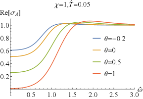
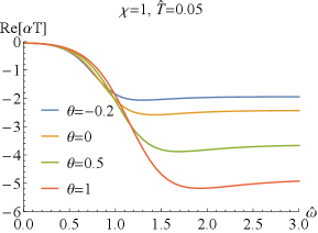
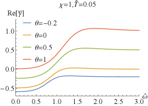
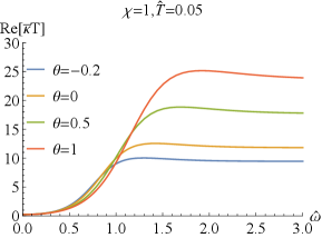
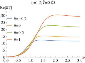
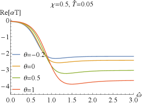
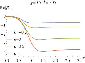
which can easily deduced from the EOMs (2) and the expressions of the conductivity (43). Numerically, we have also confirmed the above result. It is similar to that without coupling Bigazzi:2011ak . Especially, for , i.e., , one has and , which are clearly seen in FIG.1 and FIG.2.
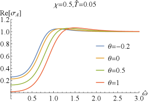
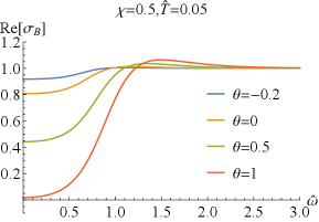
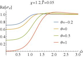
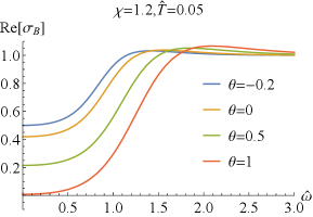
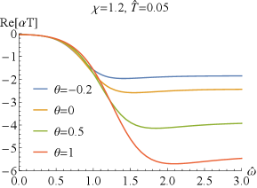
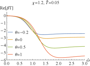
Next, we explore the properties of and . When , which has been studied in Bigazzi:2011ak , the real part of the conductivities / at low frequency exhibits a dip ( is frequency independent when .). With the doping parameter increases, the dip of becomes shallow but the one of becomes deepening (see FIG.1 and FIG.3). When is fixed, the dip in / becomes more and more deepening as increases and finally turns into a hard-gap-like when is achieved, which is independent of the doping . If we further tune larger such that it is beyond the unity, the DC conductivities of / will be negative, which violate the positive definiteness of the conductivity. Therefore, the positive definiteness of the conductivity imposes a constraint on the coupling parameter . Here, we shall constrain in the range of . Some higher derivative coupling terms also lead to the violation of the positive definiteness of the conductivity Witczak-Krempa:2013aea ; Fu:2017oqa ; Gouteraux:2016wxj ; Baggioli:2016pia .
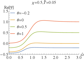
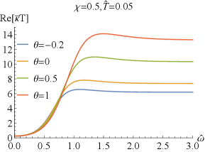
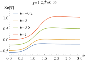
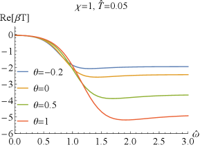
Further, we report the real part of and of the thermal conductivity for sample and in FIG.4. We find that exhibits a dip at low frequency and approaches a constant at high frequency. At full frequency, increases as increases. While converges to zero in the limit of independently of the doping and the coupling , which means that the DC thermal conductivity vanishes. As the frequency increases, the thermal conductivities with different and increase and separate out, and then approaches different constant value depending on and . With the increase of or , this constant value increases.
V Conclusions and discussions
In this paper, we construct a holographic gravity model of two gauge fields with a coupling between them, which corresponds to a two-currents model. An analytical black brane solution is obtained. Also we briefly discuss the thermodynamics. When this coupling is introduced, the expressions of conductivities for holographic two-currents model without coupling studied in Bigazzi:2011ak are no longer applicable. By the standard holographic renormalized procedure, we work out the expressions of conductivities with coupling (see Eqs.(43)). We find that the expressions of conductivities are directly related to the coupling parameter . When , they reduce to that without coupling in Bigazzi:2011ak . The expressions of conductivities for holographic two-currents model with coupling are the main topic of our present paper. Our results are also applicable for the holographic two-currents superconductor model with couple or other extension models.
As an application, then we briefly discuss the properties of the conductivities of this holographic two-currents model with coupling. An interesting property is that as the coupling increases, the dip at low frequency in / becomes deepening and finally turns into a hard-gap-like when , which is independent of the doping . Some monotonic behaviors of the conductivities are also discussed.
Along this direction, there are lots of works deserving further exploration. For example, we can add a charged complex scalar field to study the superconducting instability and the properties of the conductivities. Also it shall be surely interesting to implement the momentum dissipation into our system with coupling and study the properties of the conductivities.
Acknowledgements.
This work is supported by the Natural Science Foundation of China under Grant Nos. 11775036, 11905182 and Fok Ying Tung Education Foundation under Grant No. 171006. Guoyang Fu is supported by the Postgraduate Research & Practice Innovation Program of Jiangsu Province (KYCX20_2973). J. P. Wu is also supported by Top Talent Support Program from Yangzhou University.References
- (1) J. M. Maldacena, “The Large N limit of superconformal field theories and supergravity,” Adv. Theor. Math. Phys. 2, 231 (1998) [hep-th/9711200].
- (2) S. S. Gubser, I. R. Klebanov and A. M. Polyakov, “Gauge theory correlators from noncritical string theory,” Phys. Lett. B 428, 105 (1998) [hep-th/9802109].
- (3) E. Witten, “Anti-de Sitter space and holography,” Adv. Theor. Math. Phys. 2, 253 (1998) [hep-th/9802150].
- (4) O. Aharony, S. S. Gubser, J. M. Maldacena, H. Ooguri and Y. Oz, “Large N field theories, string theory and gravity,” Phys. Rept. 323, 183 (2000) [hep-th/9905111].
- (5) S. A. Hartnoll, C. P. Herzog and G. T. Horowitz, “Building a Holographic Superconductor,” Phys. Rev. Lett. 101 (2008) 031601. [arXiv:0803.3295 [hep-th]].
- (6) A. Donos and S. A. Hartnoll, “Interaction-driven localization in holography,” Nature Phys. 9 (2013), 649-655 [arXiv:1212.2998 [hep-th]].
- (7) Y. Ling, C. Niu, J. Wu, Z. Xian and H. b. Zhang, “Metal-insulator Transition by Holographic Charge Density Waves,” Phys. Rev. Lett. 113, 091602 (2014) [arXiv:1404.0777 [hep-th]].
- (8) H. Liu, J. McGreevy and D. Vegh, “Non-Fermi liquids from holography,” Phys. Rev. D 83, 065029 (2011) [arXiv:0903.2477 [hep-th]].
- (9) E. Kiritsis and L. Li, “Holographic Competition of Phases and Superconductivity,” JHEP 1601, 147 (2016) [arXiv:1510.00020 [cond-mat.str-el]].
- (10) M. Baggioli and M. Goykhman, “Under The Dome: Doped holographic superconductors with broken translational symmetry,” JHEP 01 (2016), 011 [arXiv:1510.06363 [hep-th]].
- (11) W. Huang, G. Fu, D. Zhang, Z. Zhou and J. P. Wu, “Doped holographic fermionic system,” Eur. Phys. J. C 80 (2020), 608 [arXiv:2002.03343 [hep-th]].
- (12) F. Bigazzi, A. L. Cotrone, D. Musso, N. Pinzani Fokeeva and D. Seminara, “Unbalanced Holographic Superconductors and Spintronics,” JHEP 1202, 078 (2012) [arXiv:1111.6601 [hep-th]].
- (13) N. Iqbal, H. Liu, M. Mezei and Q. Si, “Quantum phase transitions in holographic models of magnetism and superconductors,” Phys. Rev. D 82 (2010), 045002 [arXiv:1003.0010 [hep-th]].
- (14) M. Rogatko and K. I. Wysokinski, “Two interacting current model of holographic Dirac fluid in graphene,” Phys. Rev. D 97 (2018) no.2, 024053 [arXiv:1708.08051 [hep-th]].
- (15) M. Rogatko and K. I. Wysokinski, “Conductivity bound of the strongly interacting and disordered graphene from gauge/gravity duality,” Phys. Rev. D 101 (2020) no.4, 046019 [arXiv:2002.02177 [hep-th]].
- (16) Y. Seo, G. Song, P. Kim, S. Sachdev and S. J. Sin, “Holography of the Dirac Fluid in Graphene with two currents,” Phys. Rev. Lett. 118 (2017) no.3, 036601 [arXiv:1609.03582 [hep-th]].
- (17) N. F. Mott, “The electrical Conductivity of Transition Metals,” Proc. R. Soc. Lond. A 153, 699 (1936).
- (18) N. F. Mott, “The Resistance and Thermoelectric Properties of the Transition Metals,” Proc. R. Soc. Lond. A 156, 368 (1936).
- (19) Y. Ling, P. Liu and J. P. Wu, “A novel insulator by holographic Q-lattices,” JHEP 02 (2016), 075 [arXiv:1510.05456 [hep-th]].
- (20) Y. Ling, P. Liu, J. P. Wu and M. H. Wu, “Holographic superconductor on a novel insulator,” Chin. Phys. C 42 (2018) no.1, 013106 [arXiv:1711.07720 [hep-th]].
- (21) Y. Ling and M. H. Wu, “The instability of black holes with lattices,” [arXiv:2009.00510 [hep-th]].
- (22) Y. Ling, P. Liu and J. P. Wu, “Characterization of Quantum Phase Transition using Holographic Entanglement Entropy,” Phys. Rev. D 93 (2016) no.12, 126004 [arXiv:1604.04857 [hep-th]].
- (23) J. Tarrio and S. Vandoren, “Black holes and black branes in Lifshitz spacetimes,” JHEP 1109, 017 (2011) [arXiv:1105.6335 [hep-th]].
- (24) M. Alishahiha, E. O Colgain and H. Yavartanoo, “Charged Black Branes with Hyperscaling Violating Factor,” JHEP 11 (2012), 137 [arXiv:1209.3946 [hep-th]].
- (25) S. S. Gubser, F. D. Rocha, “Peculiar properties of a charged dilatonic black hole in ”, Phys. Rev. D 81, 046001 (2010), [arXiv:0911.2898 [hep-th]].
- (26) J. Erdmenger, V. Grass, P. Kerner and T. H. Ngo, “Holographic Superfluidity in Imbalanced Mixtures,” JHEP 08 (2011), 037 [arXiv:1103.4145 [hep-th]].
- (27) A. Dutta and S. K. Modak, “Holographic entanglement entropy in imbalanced superconductors,” JHEP 01 (2014), 136 [arXiv:1305.6740 [hep-th]].
- (28) D. Correa, N. Grandi and A. Hernandez, “Doped Holographic Superconductor in an External Magnetic Field,” JHEP 19 (2020), 085 [arXiv:1905.05132 [hep-th]].
- (29) D. Musso, “Competition/Enhancement of Two Probe Order Parameters in the Unbalanced Holographic Superconductor,” JHEP 06 (2013), 083 [arXiv:1302.7205 [hep-th]].
- (30) J. Alsup, E. Papantonopoulos and G. Siopsis, “A Novel Mechanism to Generate FFLO States in Holographic Superconductors,” Phys. Lett. B 720 (2013), 379-384 [arXiv:1210.1541 [hep-th]].
- (31) A. J. Hafshejani and S. A. Hosseini Mansoori, “Unbalanced St ckelberg holographic superconductors with backreaction,” JHEP 01 (2019), 015 Z[arXiv:1808.02628 [hep-th]].
- (32) S. Grozdanov, A. Lucas, S. Sachdev and K. Schalm, “Absence of disorder-driven metal-insulator transitions in simple holographic models,” Phys. Rev. Lett. 115 (2015) no.22, 221601 [arXiv:1507.00003 [hep-th]].
- (33) M. M. Caldarelli, A. Christodoulou, I. Papadimitriou and K. Skenderis, “Phases of planar AdS black holes with axionic charge,” JHEP 1704, 001 (2017) [arXiv:1612.07214 [hep-th]].
- (34) A. Fert and I. A. Campbell, “Two-Current Conduction in Nickel,” Phys. Rev. Lett. 21, 1190 (1968).
- (35) P. C. van Son, H. van Kempen and P. Wyder, “Boundary Resistance of the Ferromagnetic-Nonferromagnetic Metal Interface,” Phys. Rev. Lett. 58, 2271 (1987).
- (36) M. Johnson and R. H. Silsbee, “Thermodynamic analysis of interfacial transport and of the thermomagnetoelectric system,” Phys. Rev. B 35, 4959 (1987).
- (37) W. Witczak-Krempa, “Quantum critical charge response from higher derivatives in holography,” Phys. Rev. B 89 (2014) no.16, 161114 [arXiv:1312.3334 [cond-mat.str-el]].
- (38) G. Fu, J. P. Wu, B. Xu and J. Liu, “Holographic response from higher derivatives with homogeneous disorder,” Phys. Lett. B 769 (2017), 569-574 [arXiv:1705.06672 [hep-th]].
- (39) B. Gouteraux, E. Kiritsis and W. J. Li, “Effective holographic theories of momentum relaxation and violation of conductivity bound,” JHEP 04 (2016), 122 [arXiv:1602.01067 [hep-th]].
- (40) M. Baggioli, B. Gouteraux, E. Kiritsis and W. J. Li, “Higher derivative corrections to incoherent metallic transport in holography,” JHEP 03 (2017), 170 [arXiv:1612.05500 [hep-th]].