Hitting primes by dice rolls
Abstract.
Let be an infinite sequence of rolls of independent fair dice. For an integer , let be the smallest so that there are integers for which is a prime. Therefore, is the random variable whose value is the number of dice rolls required until the accumulated sum equals a prime times. It is known that the expected value of is close to . Here we show that for large , the expected value of is , where the -term tends to zero as tends to infinity. We also include some computational results about the distribution of for .
Keywords: characteristic polynomial, Chernoff inequality, combinatorial probability, hitting time, Prime Number Theorem.
MSC2020 subject classifications: 60C05, 11A41, 60G40.
1. Results
Let be an infinite sequence of rolls of independent fair dice. Thus the are independent, identically distributed random variables, each uniformly distributed on the integers . For each put . The sequence hits a positive integer if there exists an so that . In that case it hits in step .
For any positive integer , let be the random variable whose value is the smallest so that the sequence hits primes during the first steps ( if there is no such , but it is easy to see that with probability there is such ). The random variable is introduced and studied in [1], see also [4], [3] for several variants and generalizations.
Here we consider the random variable for larger values of , focusing on the estimate of its expectation.
1.1. Computational results
This article is accompanied by a Maple package PRIMESk, available from
https://sites.math.rutgers.edu/~zeilberg/mamarim/mamarimhtml/primesk.html ,
where there are also numerous output files.
Using our Maple package, we computed the following values of the expectation of for .
The table suggests that the asymptotic value of this expectation is , where the -term tends to zero as tends to infinity, and the logarithm here and throughout the manuscript is in the natural basis. This is confirmed in the results stated in the next subsection and proved in Section 2.
The value of the standard deviation of for is given in the following table.
The value of the skewness of for is given in the following table.
The value of the kurtosis of for is given in the following table.
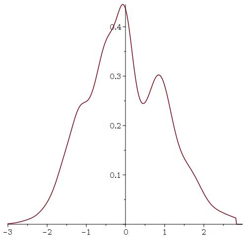
We end this section with some figures and a table of the scaled probability density functions for the number of rolls of a fair die until visiting the primes times for various values. (Recall that the scaled version of a random variable with expectation and variance is ).
| Expectation | Standard Deviation | Skewness | Kurtosis | |
|---|---|---|---|---|


Based on the available data above, the argument described in the next section, and the known results about the function which is the number of primes that do not exceed , a possible guess for a more precise expression for may be . This is also roughly consistent with the computational evidence.
1.2. Asymptotic results
In the next section we prove the following two results.
Theorem 1.1.
For any fixed positive reals there exists so that for all the probability that is smaller than .
Theorem 1.2.
For any fixed and any , the expected value of the random variable satisfies .
2. Proofs
In all proofs we omit all floor and ceiling signs whenever these are not crucial, in order to simplify the presentation.
Lemma 2.1.
There are fixed positive and so that the following holds. Let be a random sequence of independent rolls of fair dice. For any positive integer , let denote the probability that hits . Then , that is, as grows, converges to the constant with an exponential rate.
Proof.
Define , and note that for every ,
Indeed, hits if and only if the last number it hits before is for some , and the die rolled after that gives the value . The probability of this event for each specific value of is , providing the equation above. (Note that the definition of the initial values is consistent with this reasoning, as before any dice rolls the initial sum is ). Thus, the sequence satisfies the homogeneous linear recurrence relation given above. The characteristic polynomial of that is
One of the roots of this polynomial is , and its multiplicity is as the derivative of does not vanish at . It is also easy to check that the absolute value of each of the other roots , of is at most for some absolute positive constant . Therefore, there are constants so that
implying that
for some absolute constant . It remains to compute the value of . By the last estimate, for any positive ,
Note that the sum is the expected number of integers in hit by the sequence .
For each fixed , is a sum of independent identically distributed random variables, each uniform on . By the standard estimates for the distribution of sums of independent bounded random variables, see., e.g., [2], Theorem A.1.16, this sum is very close to with high probability. Therefore for large the expectation considered above is . Dividing by and taking the limit as tends to infinity shows that , completing the proof. ∎
Note that the lemma above implies that there exists an absolute positive constant so that for any (large) integer the following holds:
| (1) |
It will be convenient to apply this estimate later.
Let denote the number of primes in hit by . In the next lemma we use the letters and to represent ”hit” and ”not-hit”, respectively.
Lemma 2.2.
For any sequence of integers that satisfy and for all , where is the constant from (1), and for every the following holds. Let be the number of coordinates of . Then,
where
Proof.
The probability of the event is a product of terms. The first term is the probability that hits (if ) or the probability that does not hit (if ). Note that since this probability is in the first case and in the second case, where both and are at most .
The second term in the product is the conditional probability that hits (if ), or that it does not hit (if ), given the first value it hit in the interval . If , this first value is itself, and then the probability to hit is exactly . If , then this first value is one of the possibilities for some . Subject to hitting , the conditional probability to hit is exactly , which by the assumption on the difference , is very close to . By the law of total probability it follows that in any case the conditional probability to hit is and the conditional probability not to hit it is where the absolute value of and of is at most . Continuing in this manner we get a product of terms, of which are very close to and are very close to , where the product of all error terms is of the form for some . This completes the proof of the lemma. ∎
Proposition 2.3.
For any sequence of positive integers and any
for some absolute positive constant .
Proof.
Split into subsequences, where subsequence number consists of all with index where is the constant from (1). Note that the difference between any two distinct elements in the same subsequences is at least and that each of these subsequences can contain at most one element smaller than . Each one of the subsequences contains elements . In each subsequence, the probability to deviate in absolute value from hits by more than can be bounded by the Chernoff’s bound for binomial distributions, up to a factor of . Indeed, Lemma 2.2 shows that the contribution of each term does not exceed the contribution of the corresponding term for the binomial random variable with parameters and by more than a factor of . Note that although each subsequence may contain one element smaller than , the contribution of this single element to the deviation is negligible and can be ignored. Plugging in the standard bound, see, e.g. [2], Theorem A.1.16, we get that the probability of the event considered is at most
for appropriate absolute constants , . Here we used the fact that since is large the constant can be swallowed by the choice of . Therefore, the probability to deviate in at least one of the subsequences by more than is at most
where in the last inequality we used again the fact that . ∎
Recall that is the minimum so that hits primes in the first steps.
Corollary 2.4.
(1) If and , then
(2) If and then
Proof.
(1) The event means that the number of primes that are at most and are hit by the infinite sequence of the initial sums of dice rolls is a least . Therefore, if , we have
where the last inequality follows from Proposition 2.3.
Corollary 2.5.
(1) For a given (large) , let be the smallest integer so that
Then for any satisfying , where ,
for some absolute constant .
(2) For a given (large) and for let be the smallest integer so that
Then for any satisfying , where
Proof.
(1) If both events and do not occur, then the event does not occur. Therefore, for we have
where the last inequality follows from Chernoff’s bound and the first part of Corollary 2.4. Note that here and therefore the corollary can be applied.
(2) Similarly, if both events and do not occur, then the event does not occur. Therefore, for , we have
where the last inequality follows again from Chernoff’s bound and the second part of Corollary 2.4. Indeed the corollary can be applied since it is not difficult to check that for large and any ,
∎
Proof of Theorem 1.1: Note that by the Prime Number Theorem in the first part of Corollary 2.5,
Taking and letting be the largest integer so that it follows from this first part that and that the probability that is smaller than is smaller than some negative power of , that is, tends to as tends to infinity.
Similarly, substituting in the second part of the corollary and letting be the smallest integer so that it is easy to see that is also (since
by the Prime Number Theorem). By the second part of the corollary the probability that is larger than is smaller than any fixed negative power of , and hence tends to as tends to infinity. Therefore is with probability tending to as tends to infinity, completing the proof of the theorem.
Proof of Theorem 1.2: The expectation of is the sum over all positive integers , of the probabilities . Taking and defining and as before we break this sum into three parts,
and
By the first part of Corollary 2.5 each summand in the first sum is and therefore , as the number of summands is , since By the second part of the corollary (applied to an appropriately chosen sequence of and ) it is not difficult to check that the infinite sum is only . Indeed, it is possible, for example, to choose and for all . The corresponding value of for each is defined as the smallest integer satisfying . Taking we can apply the estimate in the second part of the corollary to all values of satisfying . The sum of the probabilities for these values of is thus at most for , and at most for each . The sum of all these quantities is smaller than any fixed negative power of , and is therefore , as needed.
The sum is a sum of at most terms, and each of them is at most , implying that , since both and are , and . This completes the proof of the theorem.
3. Concluding remarks and extensions
-
•
Extensions for biased -sided dice and arbitrary subsets of the integers. The proofs in the previous section use very little of the specific properties of the primes and the specific distribution of each . It is easy to extend the result to any -sided dice with an arbitrary discrete distribution on in which the values obtained with positive probabilities do not have any nontrivial common divisor. The constants and will then have to be replaced by the expectation of the random variable and by its reciprocal, respectively. It is interesting to note that while for different dice the expectation of for small values of can be very different from the corresponding expectation for a standard fair die, once the die is fixed, for large the expectation is always , where the -term tends to as tends to infinity.
It is also possible to replace the primes by an arbitrary subset of the positive integers, and repeat the arguments to analyze the corresponding random variable for this case, replacing the Prime Number Theorem by the counting function of . We omit the details.
-
•
Heuristic suggestion for a more precise expression for . If we substitute for its approximation and repeat the analysis described here with this approximation, the more precise value for the expectation that follows is . Since at the beginning there are some fluctuations, we tried to add another constant and consider an expression of the form . Choosing and that provide the best fit for our (limited and therefore maybe overfitted) computational evidence we obtained the heuristic expression For the record, here are the ratios of for , respectively:
.
One can also replace by the more precise approximation for , but the difference between these two estimates does not change the expression obtained for in a significant way.
Acknowledgment Noga Alon is supported in part by NSF grant DMS-2154082. Yaakov Malinovsky is supported in part by BSF grant 2020063. Lucy Martinez is supported by the NSF Graduate Research Fellowship Program under Grant No. 2233066. YM expresses gratitude to Stanislav Molchanov for suggesting that the hits on squares asymptotically follow a success probability of .
References
- [1] Noga Alon and Yaakov Malinovsky, Hitting a prime in 2.43 dice rolls (on average), The American Statistician, Volume 77 (2023), no. 3, 301-303. https://arxiv.org/abs/2209.07698
- [2] Noga Alon and Joel H. Spencer, The Probabilistic Method, Fourth Edition, Wiley, 2016, xiv+375 pp.
- [3] Shane Chern, Hitting a prime by rolling a die with infinitely many faces, The American Statistician, Volume 78 (2024), no. 3, 297-303. https://arxiv.org/abs/2306.14073
- [4] Lucy Martinez and Doron Zeilberger, How many dice rolls would it take to reach your favorite kind of number?, Maple Transactions, Volume 3 (2023), no. 3, Article 15953. https://mapletransactions.org/index.php/maple/article/view/15953