High–Resolution Observations of Prominence Plume Formation with the New Vacuum Solar Telescope

Simon et al. (1982) described the measurement methods of Doppler velocities and line broadening at two and four wavelengths in the same emission line. Taking into account the non-negligible errors, we propose a tentative determination of the three main line parameters at three wavelengths, named as 3-points method. We assume that the off–disk H$\mathrm{\alpha}$ lines are optically thin and the continua are negligible (Gouttebroze et al. 1993). This assumption is possibly satisfied over $6\,\mathrm{Mm}$ in altitude, where H$\mathrm{\alpha}$ center intensities are generally higher than the average intensities of $\pm 0.4\,\mathrm{\AA}$, which means that the integrated opacity is not large (Gouttebroze et al. 1993; Heinzel et al. 2014, 2015). After subtracting the observed stray light, we assume that off–disk H$\mathrm{\alpha}$ lines have Gaussian profiles

where $I$ is the intensity at wavelength $\lambda$, $I_{0}$ is the central intensity, $\lambda_{\mathrm{D}}$ is the central wavelength modified by a Doppler shift, and $w$ is the Gaussian width. With three off–band H$\mathrm{\alpha}$ observations, plugging wavelengths $\lambda_{1}-\lambda_{3}$ and corresponding intensities $I_{1}-I_{3}$ into Eq. (1) yields

The Doppler speed $v_{\mathrm{D}}$ is derived from

where $c$ is the light speed, $\Delta\lambda_{\mathrm{D}}$ is wavelength shift due to the Doppler effect, and $\lambda_{0}=6562.8\,\mathrm{\AA}$ is the H$\mathrm{\alpha}$ rest wavelength.

If natural broadening and collisional broadening are ignored, the Gaussian width $w$ is mainly contributed by thermal, nonthermal and instrumental broadening:

where $w_{\mathrm{instr}}$ is the instrumental broadening. The thermal velocity $v_{\mathrm{t}}$ is defined as:

$k_{\mathrm{B}}$, $T$, and $m_{\mathrm{H}}$ are the Boltzmann constant, temperature, and hydrogen mass, respectively. Because $w_{\mathrm{instr}}$ is unknown, we define $v_{\mathrm{nt}}$ as:

which actually includes the instrumental broadening. In Section 3.3, we will find that $(c/\lambda_{0})w_{\mathrm{instr}}<10\,\mathrm{km\,s^{-1}}$. $v_{\mathrm{nt}}$ maps are calculated with the assumption $T=9,500\,\mathrm{K}$ for all the off–disk structures (Chae et al. 2013). $v_{\mathrm{nt}}$ is generally used to evaluate the plasma turbulence along line of sight (LOS).

The square root of photon number or digital number (DN) is generally treated as intensity error, which assumes that received photons follow a Poisson distribution. Then we can derive the errors of $\lambda_{\mathrm{D}}$, $w$, and $I_{\mathrm{0}}$ using the error propagation formula. For example, error of $\lambda_{\mathrm{D}}$ is calculated using

where $\frac{\partial\lambda_{\mathrm{D}}}{\partial I_{j}}~{}(j=1,2,3)$ are derived from Eq. (2). Since we derive the Gaussian parameters at only three wavelengths, the measurement errors are sensitive to Doppler shifts. To evaluate the variation of $\lambda_{\mathrm{D}}$, $w$, and $I_{\mathrm{0}}$ errors with respect to the Doppler shifts $\Delta\lambda_{\mathrm{D}}$, we set a series of Gaussian profiles with $I_{\mathrm{0}}=2000\,\mathrm{DN}$ and $w=0.35,0.5\,\mathrm{\AA}$ according to our observations. With varying $\Delta\lambda_{\mathrm{D}}$, Gaussian profiles and $I_{1}-I_{3}$ are determined, then we can calculate the errors of $\lambda_{\mathrm{D}}$ (using Eq. (7)), $w$, and $I_{\mathrm{0}}$. The results are plotted in Figs. 2(a)–(c). They show that all the parameter errors vary gently when $\Delta\lambda_{\mathrm{D}}<0.4\,\mathrm{\AA}$ and vary faster beyond it, which is due to the fact that the chosen wavelengths are within $0.4\,\mathrm{\AA}$. Besides, the wider profile is less sensitive to Doppler shifts than the thinner one. Note that $0.4\,\mathrm{\AA}$ corresponds to a shift of $\sim 18\,\mathrm{km\,s^{-1}}$, and $w=0.35,0.5\,\mathrm{\AA}$ correspond to $v_{\mathrm{nt}}=10,19\,\mathrm{km\,s^{-1}}$, respectively, when $T=9500\,\mathrm{K}$ for H$\mathrm{\alpha}$ line. This method does not allow any degree of freedom in measurement, so we cannot evaluate how much the observed H$\mathrm{\alpha}$ lines deviate from Gaussian profiles.

The reliability of measured $w$ and $I_{\mathrm{0}}$ also depends on the estimation of stray light, which is mainly due to the scattering of solar disk emission by Earth’s atmosphere and the instrument. Figure 2(d) shows the deviation of measured $w$ from the assumed values (noted in the legend in the units of $\mathrm{\AA}$) versus continuum. Negative continuum value means that stray light is overestimated, in which case $w$ is underestimated, and vice versa. This effect gets more significant when there is a Doppler shift (dotted blue curve). In this work, the stray light is evaluated at a clear region beyond the prominence (the white box in Fig. 2(e)). The stray light is a function of height (plus signs in Fig. 2(f)), and its distribution is fitted by a power law with a negative power index (solid red curve). The calculation of spectral parameters is performed on bright H$\mathrm{\alpha}$ structures above $6.9\,\mathrm{Mm}$ from the solar limb (dashed blue line). In this work, we estimate the intensity error from two components: one is the square root of digital number, the other is the standard deviation of stray light after subtracting the fitting curve.

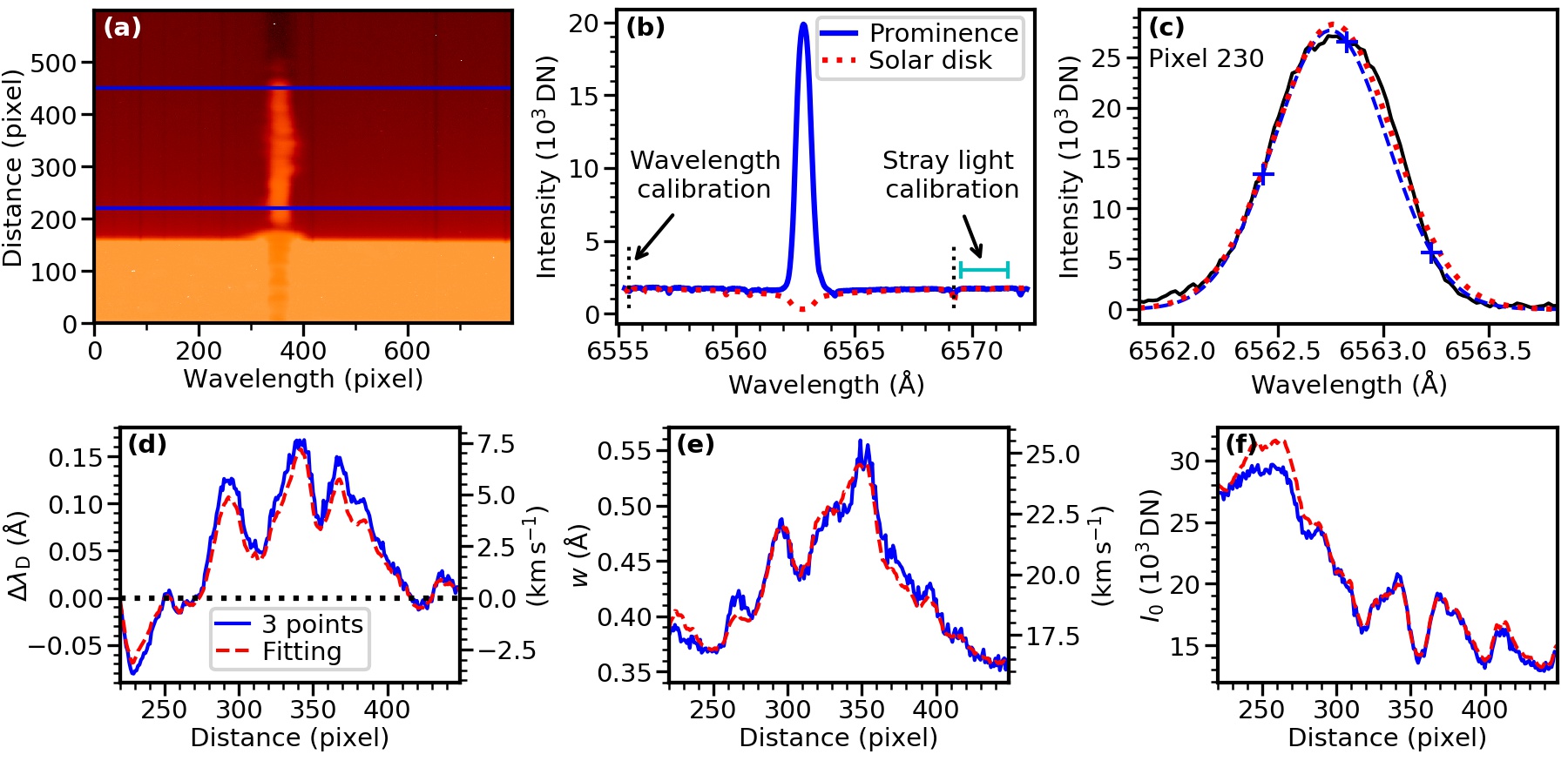
Gaussian fitting is widely used to derive spectral parameters for emission lines. To test the reliability of the 3-points method, we compared it with Gaussian fitting using a set of H$\mathrm{\alpha}$ spectral data of a prominence observed with the Multi–wavelength Spectrometer on the NVST (Wang et al. 2013). Figure 3(a) shows the spectral image with X-axis wavelength and Y-axis distance in units of pixel. The region between two blue lines is taken to make the average H$\mathrm{\alpha}$ profile as shown in Fig. 3(b). Before performing Gaussian parameter measurements on the data, wavelength and stray light calibrations are necessary. The faint absorption lines on both sides of the H$\mathrm{\alpha}$ profile result from the scattering of solar disk light, by which we can determine the wavelength. We adopt the spectral data observed by the Fourier Transform Spectrometer (FTS) at the McMath/Pierce Solar Telescope (Brault 1978) as standard solar disk spectrum (dotted red curve in Fig. 3(b)), and compare them with the average prominence spectrum (solid black curve). The two reference lines for wavelength calibration are marked with vertical dotted lines, which are Si I $6555.5\,\mathrm{\AA}$ and Fe I $6569.2\,\mathrm{\AA}$, respectively. Intensity of stray light is a function of height and wavelength, and is related to solar disk radiation:

where $I_{\mathrm{SL}}$ is stray light intensity of observed prominence spectrum, $I_{\mathrm{SD}}$ represents the solar disk radiation, $d$ is height. The coefficient $C(d)$ is determined using the wavelength range marked with cyan lines, where we assume that the observed prominence radiation is from scattering of solar disk light totally. In Fig. 3(b), the dotted red curve is FTS data multiplied by the coefficient, hence it represents the stray light intensity of the prominence spectrum.

After wavelength calibration and stray light being subtracted, the solid black curve in Fig. 3(c) is the prominence H$\mathrm{\alpha}$ line at distance 230 pixel, as an example. We didn’t plot error bars because most errors are too small to show. The 3 plus symbols mark the points at 0 and $\pm 0.4\,\mathrm{\AA}$, and the dashed blue curve is the result of the 3-points method. The dotted red curve is the result of Gaussian fitting using all the observed points. The two calculated profiles are similar. The derived $\Delta\lambda_{\mathrm{D}}$, $w$, and $I_{0}$ along distance are shown in Figs. 3(d)–(f), respectively, where solid blue curves are the results of the 3-points method, and dashed red curves are that of Gaussian fitting. The maximum difference of $\Delta\lambda_{\mathrm{D}}$ of the two methods is $0.031\,\mathrm{\AA}$ (Doppler velocity $\sim 1.4\,\mathrm{km\,s^{-1}}$); that of $w$ is $0.026\,\mathrm{\AA}$ (relative difference 5.9%); that of $I_{0}$ is $826\,\mathrm{DN}$ (relative difference 4.1%).

A knowledge of the three–dimensional structure is important to understand the two–dimensional projection of the prominence (Gunár et al. 2018). Four days before the observation, the target prominence was seen as a dark filament that had the orientation of northeast–southwest (NE–SW) and east–west (E–W) on the two sides of the longitude $45^{\circ}$ (Fig. 1(a)). During the four days, the Sun has rotated about $53^{\circ}$, thus the prominence observed on 2018 November 10 is mainly oriented NE–SW, and part of E–W oriented prominence is blocked by the NE–SW part (Fig. 1(b)). The prominence is embedded in a coronal cavity and large–scale bright loops in AIA $171\,\mathrm{\AA}$ filtergram ($\sim 0.8\,\mathrm{MK}$, Fig. 1(c)). Different from the usual “tennis racquet” shaped coronal cavities (Berger et al. 2011; Gibson 2018), the cavity in our observations is relatively wide and low. The prominence is bright in AIA 304, 171, and $131\,\mathrm{\AA}$ (Figs. 1(b)–(d)), and the prominence bubble and plumes are shielded in these channels by the PCTR. The prominence threads are dark in AIA 193 ($\sim 1.6\,\mathrm{MK}$, Fig. 1(e)) and $211\,\mathrm{\AA}$ ($\sim 2.0\,\mathrm{MK}$, Fig. 1(f)) due to continuum absorption, and the bubble and plumes are visible as bright features compared to prominence threads. The three NVST H$\mathrm{\alpha}$ spectral maps in Figs. 1(g)–(i) are shown in the same brightness scale for estimating the Doppler shifts. The bright bubble–prominence interface and dark plumes are clear at H$\mathrm{\alpha}$ $-0.4\,\mathrm{\AA}$ and center.

The formation and evolution processes of the plumes that we focus on are shown in Fig. 4. The formation of the plumes starts from the elevation of the bubble–prominence interface, and the interface gets brighter simultaneously (Figs. 4(a)–(b)). The rising interface is transformed into two plumes with a finger–shaped feature formed (Fig. 4(c)). Then the two plumes continue rising at a speed of $\sim 14\,\mathrm{km\,s^{-1}}$, and the finger gets longer (Fig. 4(d)–(e)). During the evolution of plumes, shorter and denser fingers occur firstly at the bubble–prominence interface (Fig. 4(e)), then move into the plume (Fig. 4(f)). At the late phase of the plume evolution, more fingers occur along the plume boundary (Figs. 4(g)–(h)). The plane–of–sky (POS) velocities calculated using the FLCT technique show obvious flows along the prominence boundary, including the region where fingers occur (Fig. 4(h)). The rising plumes incline leftwards, which is consistent with the flow direction. In addition, a small plume appears at lower height (Fig. 4(f)), which is also split and fingers occur between plumes (Figs. 4(g)–(h)) as the large plumes mentioned before. The finger structures have been predicted in RT instability simulations (Hillier et al. 2011; Keppens et al. 2015; Xia & Keppens 2016) and the nearly horizontal fingers were reported by Awasthi & Liu (2019).

We find that the flows along the bubble–prominence boundary (Fig. 4(h)) already exist before the plume formation, which are obvious in H$\mathrm{\alpha}$ $-0.4\,\mathrm{\AA}$ images. In the reverse and saturated H$\mathrm{\alpha}$ $-0.4\,\mathrm{\AA}$ map in Fig. 5(a), some bright knots appear along the prominence boundary, which are blue shifted (Fig. 5(c)). We synthesized time–distance diagrams along the bubble–prominence boundary (the slice in Fig. 5(a) from bottom–right side to the top–left side of the bubble), and the H$\mathrm{\alpha}$ $-0.4\,\mathrm{\AA}$ and Doppler velocity diagrams are shown in Figs. 5(b) and (d), respectively. The top part of the slice misses the prominence at $\sim$06:25 UT, which is due to the elevation of the prominence during the plume formation. Obvious flows occur around 06:17 UT, $\sim 10$ minutes before the plume formation. Almost all the knots flow from the lower right side to the upper left side, and are blue shifted. Such motions continue till the end of the diagram, including the period during which the new plume occurs. Their speeds are non–uniform, generally within $12\,\mathrm{km\,s^{-1}}$ on POS (Fig. 5(b)) and within $8\,\mathrm{km\,s^{-1}}$ along LOS (Fig. 5(d)). A typical knot is marked in Figs. 5(a) and (c). Its POS velocity is $v_{\mathrm{POS}}=8.9\pm 0.8\,\mathrm{km\,s^{-1}}$ and the Doppler velocity is $v_{\mathrm{LOS}}=-6.8\pm 5.0\,\mathrm{km\,s^{-1}}$ (toward us). Therefore, the total speed is $v_{\mathrm{total}}=11.2\pm 3.1\,\mathrm{km\,s^{-1}}$, and the angle with POS is $37\degr\pm 20\degr$.

Figure 4 shows the brightening enhancement at plume fronts during their formation. Their $v_{\mathrm{D}}$ and $v_{\mathrm{nt}}$ maps are plotted in Fig. 6. Compared with the initial maps (Figs. 6(a) and (d)), $v_{\mathrm{D}}$ at the plume fronts increases significantly and reaches $-16\pm 10\,\mathrm{km\,s^{-1}}$. At the same time, the region also gets more turbulent and $v_{\mathrm{nt}}$ is $>26\pm 10\,\mathrm{km\,s^{-1}}$ after subtracting the instrumental broadening ($(c/\lambda_{0})w_{\mathrm{instr}}$ is expected to be $<10\,\mathrm{km\,s^{-1}}$ from Figs. 6(d)–(f)). When plasma temperature is in the range of $6000-15\,000\,\mathrm{K}$, the corresponding sound speed is $\lesssim 13-20\,\mathrm{km\,s^{-1}}$. Hence, the large $v_{\mathrm{nt}}$ already exceeds the local sound speed.

We check other three plume cases in Fig. 7 and find that the enhancements of brightening, blue shifts, and turbulence commonly occur at the plume fronts. The regions of interest are marked with arrows. In the first event (left column), the nearby two plumes are relatively large and the obvious blue shifts and large $v_{\mathrm{nt}}$ are distributed along the plume fronts. In the latter two cases (middle and right columns), the plumes are relatively small and the turbulent regions are more compact.

References

- Awasthi & Liu (2019) Awasthi, A. K., & Liu, R. 2019, Frontiers in Physics, 7, 218
- Berger et al. (2008) Berger, T. E., Shine, R. A., Slater, G. L., et al. 2008, ApJ, 676, L89
- Berger et al. (2010) Berger, T. E., Slater, G., Hurlburt, N., et al. 2010, ApJ, 716, 1288
- Berger et al. (2017) Berger, T., Hillier, A., & Liu, W. 2017, ApJ, 850, 60
- Berger et al. (2011) Berger, T., Testa, P., Hillier, A., et al. 2011, Nature, 472, 197
- Brault (1978) Brault, J. W. 1978, in Future solar optical observations needs and constraints, ed. G. Godoli, Vol. 106, 33
- Chae et al. (2013) Chae, J., Park, H., & Song, D. 2013, Proceedings of the International Astronomical Union, 8, 85
- Dudík et al. (2012) Dudík, J., Aulanier, G., Schmieder, B., Zapiór, M., & Heinzel, P. 2012, ApJ, 761, 9
- Fisher & Welsch (2008) Fisher, G. H., & Welsch, B. T. 2008, in Astronomical Society of the Pacific Conference Series, Vol. 383, Subsurface and Atmospheric Influences on Solar Activity, ed. R. Howe, R. W. Komm, K. S. Balasubramaniam, & G. J. D. Petrie, 373
- Gibson (2018) Gibson, S. E. 2018, Living Reviews in Solar Physics, 15, 7
- Gouttebroze et al. (1993) Gouttebroze, P., Heinzel, P., & Vial, J. C. 1993, A&AS, 99, 513
- Gunár et al. (2018) Gunár, S., Dudík, J., Aulanier, G., Schmieder, B., & Heinzel, P. 2018, ApJ, 867, 115
- Gunár et al. (2014) Gunár, S., Schwartz, P., Dudík, J., et al. 2014, A&A, 567, A123
- Guo et al. (2014) Guo, L. J., Huang, Y. M., Bhattacharjee, A., & Innes, D. E. 2014, ApJ, 796, L29
- Heinzel et al. (2015) Heinzel, P., Schmieder, B., Mein, N., & Gunár, S. 2015, ApJ, 800, L13
- Heinzel et al. (2014) Heinzel, P., Zapiór, M., Oliver, R., & Ballester, J. L. 2014, A&A, 562, A103
- Hillier (2018) Hillier, A. 2018, Reviews of Modern Plasma Physics, 2, 1
- Hillier et al. (2012) Hillier, A., Hillier, R., & Tripathi, D. 2012, ApJ, 761, 106
- Hillier et al. (2011) Hillier, A., Isobe, H., Shibata, K., & Berger, T. 2011, ApJ, 736, L1
- Keppens et al. (2015) Keppens, R., Xia, C., & Porth, O. 2015, ApJ, 806, L13
- Labrosse et al. (2010) Labrosse, N., Heinzel, P., Vial, J. C., et al. 2010, Space Sci. Rev., 151, 243
- Lemen et al. (2012) Lemen, J. R., Title, A. M., Akin, D. J., et al. 2012, Sol. Phys., 275, 17
- Li et al. (2018) Li, D., Shen, Y., Ning, Z., Zhang, Q., & Zhou, T. 2018, ApJ, 863, 192
- Liu et al. (2014) Liu, Z., Xu, J., Gu, B.-Z., et al. 2014, Research in Astronomy and Astrophysics, 14, 705
- Pesnell et al. (2012) Pesnell, W. D., Thompson, B. J., & Chamberlin, P. C. 2012, Sol. Phys., 275, 3
- Shen et al. (2015) Shen, Y., Liu, Y., Liu, Y. D., et al. 2015, ApJ, 814, L17
- Simon et al. (1982) Simon, G., Mein, P., Vial, J. C., Shine, R. A., & Woodgate, B. E. 1982, A&A, 115, 367
- Vial & Engvold (2015) Vial, J.-C., & Engvold, O. 2015, Solar Prominences, Vol. 415
- Wang et al. (2013) Wang, R., Xu, Z., Jin, Z.-Y., et al. 2013, Research in Astronomy and Astrophysics, 13, 1240
- Xia & Keppens (2016) Xia, C., & Keppens, R. 2016, ApJ, 825, L29