Higher-order Topological Hyperbolic Lattices
Abstract
A hyperbolic lattice allows for any -fold rotational symmetry, in stark contrast to a two-dimensional crystalline material, where only twofold, threefold, fourfold or sixfold rotational symmetry is permitted. This unique feature motivates us to ask whether the enriched rotational symmetry in a hyperbolic lattice can lead to any new topological phases beyond a crystalline material. Here, by constructing and exploring tight-binding models in hyperbolic lattices, we theoretically demonstrate the existence of higher-order topological phases in hyperbolic lattices with eight-fold, twelve-fold, sixteen-fold or twenty-fold rotational symmetry, which is not allowed in a crystalline lattice. Since such models respect the combination of time-reversal symmetry and -fold (8, 12, 16 or 20) rotational symmetry, zero-energy corner modes are protected. For the hyperbolic {8,3} lattice, we find a higher-order topological phase with a finite edge energy gap and a gapless phase. Our results thus open the door to studying higher-order topological phases in hyperbolic lattices.
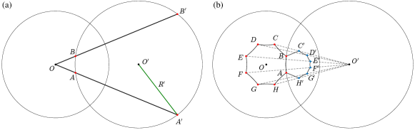
Recently, hyperbolic lattices have been experimentally realized in circuit quantum electrodynamics Houck2019nat and electric circuits Zhang2022NC ; Lenggenhager2022NC ; Boettcher2022arxiv , igniting great interest in study of various properties of hyperbolic lattices Houck2019CMP ; Park2020PRL ; Gorshkov2020PRA ; Rayan2021scia ; Matsuki2021JOP ; Rouxinol2021arxiv ; Rayan2022PNAS ; Gorshkov2022PRL ; Boettcher2022PRL ; Thomale2022PRB ; Urwyler2022arxiv ; Zhou2022PRB ; Mao2022arxiv ; Bzdusek2022PRB ; Mosseri2022PRB , such as topological properties, hyperbolic band theory and flat band properties. Different from a hyperbolic lattice, it is a well-known fact that only twofold, threefold, fourfold or sixfold rotational symmetry is permitted in two-dimensional (2D) crystalline materials. In other words, one can only use regular -sided polygons with , or to tessellate the 2D Euclidean plane. However, for a hyperbolic lattice with constant negative curvature, such a restriction is lifted so that one can use regular -gons for any integer to tessellate a hyperbolic plane [see Fig. 1(a)]. As a result, any -fold rotational symmetry can be realized in a hyperbolic lattice. This leads to a natural question of whether the enriched rotational symmetry of a hyperbolic lattice will result in any new topological phases beyond crystalline systems.
Recent generalizations of topological phases to the higher-order case provide us with an opportunity to study the effects of the enriched rotational symmetry. Different from the conventional first-order topological system, such a topological phase supports -dimensional () gapless boundary modes for an -dimensional system Taylor2017Science ; Fritz2012PRL ; ZhangFan2013PRL ; Slager2015PRB ; Brouwer2017PRL ; FangChen2017PRL ; Schindler2018SA ; Taylor2018PRB(R) ; Brouwer2019PRX ; Roy2019PRB ; Fulga2019PRL ; Yang2019PRL ; Roy2020PPR ; Xu2020PRL ; Parameswaran2020PRL ; Xu2020PPR ; Xu2020PPB ; AYang2020PRL ; Xu2020NJP ; Seradjeh2019PRB ; Wang2021PRL . For instance, a two-dimensional (2D) second-order topological insulator may support two, four or six zero-energy corner modes Taylor2017Science ; Yang2019PRL ; AYang2020PRL . Since the number of corner modes is closely related to the crystalline symmetry of a system, one thus may wonder whether the new rotational symmetry in hyperbolic lattices can allow for the existence of new higher-order topological phases that cannot exist in a crystalline material.
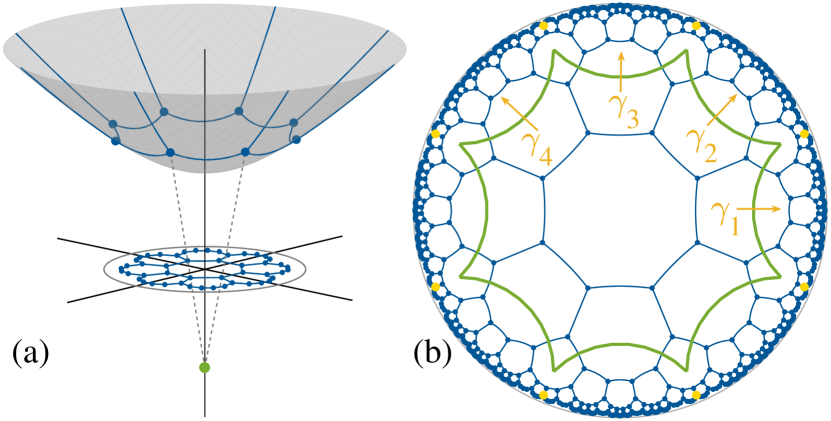
In this work, we theoretically demonstrate the existence of higher-order topological phases in hyperbolic lattices with eight-fold, twelve-fold, sixteen-fold or twenty-fold rotational symmetry by constructing and exploring tight-binding models on the lattices. Such Hamiltonians respect the combination of time-reversal symmetry and -fold (8, 12, 16 or 20) rotational symmetry, which is not allowed in a crystalline lattice. While a quasicrystal may allow for the eight-fold or twelve-fold rotational symmetry, to the best of our knowledge, it is unclear whether sixteen-fold or twenty-fold rotational symmetry can occur there Sunbook . For clarify of presentation, we mainly focus on a hyperbolic lattice where regular -gons are used to tessellate a hyperbolic plane such that each lattice site is connected to three neighboring sites [see Fig. 1(b)]. Note that for the Euclidean plane, only , and lattices can achieve the tessellation. For the hyperbolic lattice, we find a gapped and a gapless higher-order topological hyperbolic phase by numerically computing the quadrupole moment and energy band properties of a four-dimensional (4D) momentum-space Hamiltonian based on the hyperbolic band theory Rayan2021scia . We further study a Hamiltonian on a hyperbolic lattice without translational symmetry and find the existence of eight-fold degenerate zero-energy modes localized at eight corners in a phase with a finite edge energy gap. The topology of this phase is characterized by the corner charge. Interestingly, there also appears a gapless phase with vanishing edge energy gap where states near zero energy are mainly localized on the boundary of the hyperbolic lattice. In addition, the real space results also show a reentrant gapped topological phase with zero-energy corner modes, which may arise from finite-size effects. Finally, we show the existence of twelve, sixteen or twenty zero-energy corner modes in a hyperbolic lattice with the corresponding rotational symmetry.
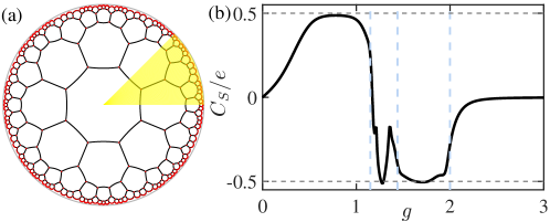
Model with hyperbolic translational symmetry.—To demonstrate the existence of higher-order topological phases in hyperbolic lattices, we will construct two types of tight-binding models in a hyperbolic lattice described by the Poincaré disk model [see Fig. 1(b)]. We start by constructing the first tight-binding model in a hyperbolic lattice with hyperbolic translational symmetry by following Ref. Urwyler2022arxiv . We first construct the onsite and hopping term inside the first unit cell [the region enclosed by the green curve in Fig. 1(b)], , where denotes the state of the th degree of freedom at the site in the th unit cell in the Poincaré disk. At each site, there are four degrees of freedom, and and with are two sets of Pauli matrices that act on these degrees of freedom. In , the first term describes the on-site energy, and the second term depicts the hopping between two neighboring connected sites inside the unit cell with the hopping matrix with , where is the polar angle of the vector from the site to site in the first unit cell. In the following, we will set the system parameters as the units of energy.
For the hopping term between the sites in the first unit cell and the sites in the neighboring four unit cells described by the set , we define it as . To ensure that the system has symmetry (here ) where is the -fold rotational operator and is the time-reversal operator, we have to consider a modified (see Supplemental Material Sec. S-2). The entire Hamiltonian can be generated by applying translational operations (generated by generators ).
When , the system respects in-plane mirror symmetry , time-reversal symmetry where is the complex conjugate operator, chiral symmetry , and thus particle-hole symmetry . Owing to the eight-fold rotational symmetry about the axis preserved by the hyperbolic lattice, the Hamiltonian also respects the eight-fold rotational symmetry where with rotating the lattice site by an angle about the axis (here ). With these internal symmetry, the system belongs to the DIII class corresponding to a topological insulator whose nontrivial phase exhibits helical edge modes. To generate a higher-order phase with corner modes, we add the term to break the time-reversal symmetry so as to open the gap of the helical modes at a boundary; this term thus acts as an edge mass term. As this term changes its sign once increases by , a corner state may arise at the location where the mass flips its sign. Since the change of sign occurs eight times, total eight corner modes may appear. While the term also breaks the symmetry, the combination of and symmetry is still conserved. The symmetry ensures that the number of corner modes must be an integer multiple of eight given the fact that if there is a zero-energy corner mode mainly localized at , then is also a zero-energy corner mode mainly localized at .
We now employ the twisted boundary conditions to construct the momentum-space Bloch Hamiltonian based on the hyperbolic band theory Rayan2021scia ; Rayan2022PNAS ; Mao2022arxiv . In the Hamiltonian, the hopping between two sites in two different unit cells which are connected by a translation operator should carry an extra phase term . We thus obtain a Hamiltonian in a four-dimensional Brillouin zone with for (see Supplemental Material Sec. S-2) .
While time-reversal symmetry is broken in the Hamiltonian , chiral symmetry is still preserved so that respects chiral symmetry. In light of the fact that the quadrupole moment Cho2019PRB ; Hughes2019PRB is protected to be quantized by chiral symmetry Xu2021PRB ; Shen2020PRL , we can utilize the quadrupole moment to characterize the topological property of spanned by two of the four momenta. Specifically, one can regard spanned by and ( and ) with the other two momenta and fixed as the momentum-space version of a Hamiltonian in an square lattice. The quadrupole moment for the occupied states is defined as Cho2019PRB ; Hughes2019PRB ; Xu2021PRB ; Shen2020PRL
| (1) |
where with being the th occupied eigenstate of (one of occupied states), and with denoting the square position of the th lattice site. Here, is the contribution from the background positive charge distribution.
To distinguish between an insulating phase and a semimetal phase, we calculate the average quadrupole moment over all fixed momenta
| (2) |
The system respects symmetry, that is, . It follows that should satisfy the following relations (see Supplemental Material Sec. S-3 for proof):
| (3) | ||||
| and |
Note that a similar relation for the Chern number has been derived in Ref. Urwyler2022arxiv . We find that is always equal to zero and thus use to characterize the topological property.
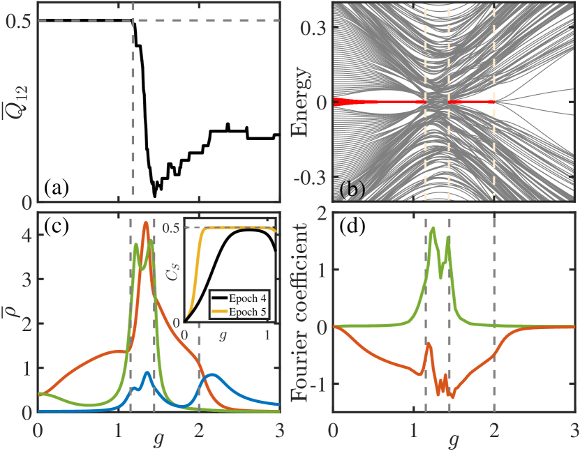
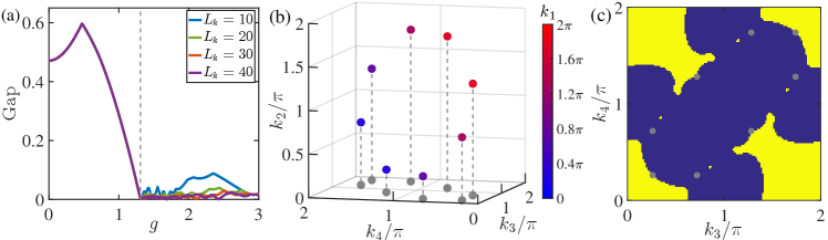
The average quadrupole moment illustrates a sharp decline from a quantized value of to a nonzero fractional value as increases as shown in Fig. 2(a), indicating the presence of two distinct phases. One phase is a higher-order topological hyperbolic insulator with . The other one is a higher-order topological hyperbolic semimetal with vanishing energy gap in the 4D momentum space footnote . In fact, there are several degenerate nodes in momentum space. In the Brillouin zone spanned by , a part has the quadrupole moment of and the other part has zero , leading to a fractional value of the average quadrupole moment (see Supplemental Material Sec. S-4). The existence of the gapless phase is in stark contrast to the higher-order phase on Euclidean square lattices where the system is always gapped as we increase the term that breaks the time-reversal symmetry Taylor2017Science ; Schindler2018SA .
Model without hyperbolic translational symmetry.—For the model with translational symmetry, while the hyperbolic band theory predicts the existence of higher-order topological phases, we find that its energy spectrum in real space changes dramatically for different system sizes possibly due to large boundary effects (see Supplemental Material Sec. S-5). We therefore construct another tight-binding model Hamiltonian in a hyperbolic lattice as
| (4) |
where denotes the state of the th degree of freedom at the site in the disk, and is the polar angle of the vector from the site to the site , rather than a modified one. This model respects the symmetry. Note that should be an integer multiple of 4 to ensure that the Hamiltonian is Hermitian.
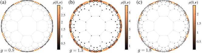
To illustrate the existence of zero-energy corner modes, we calculate the eigenenergies and eigenstates of the Hamiltonian in Eq. (4) in real space under open boundary conditions. We further compute the local density of states (DOS) defined as , where is the th component of the th eigenstate at site r with the eigenenergy .
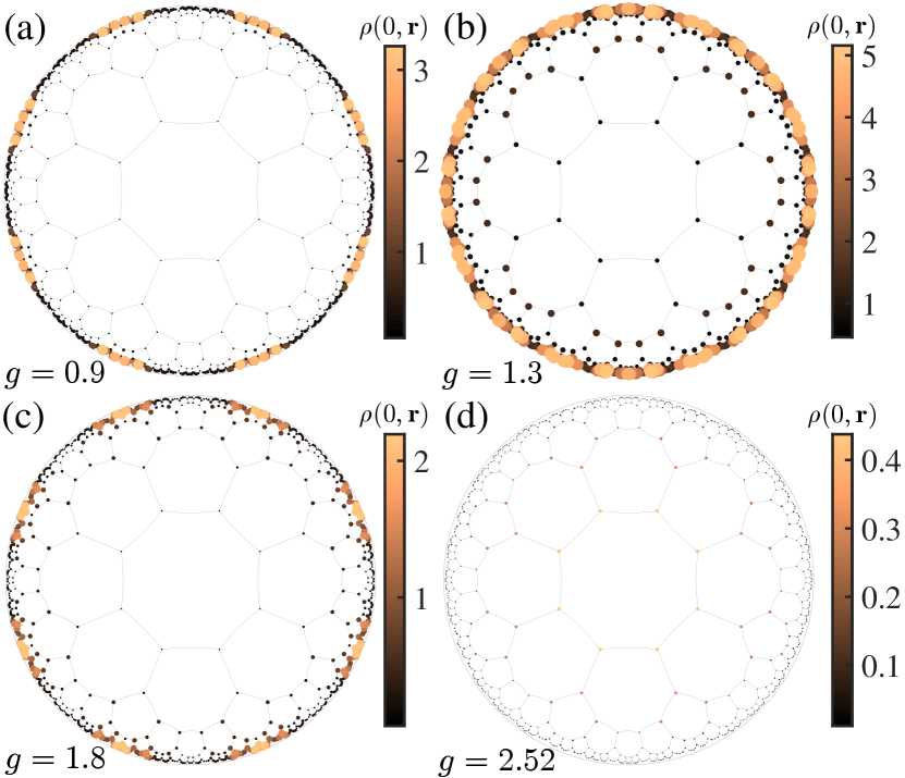
The energy spectrum in Fig. 2(b) shows the existence of eight-fold degenerate zero-energy states when . These modes are mainly localized near the corner positions on the boundary at the polar angle with as shown by the local DOS in Fig. 3(a). Such a feature is also revealed by the average local DOS near a corner and the center of an edge (e.g., ) (here an edge refers to the collection of the boundary sites between two nearest neighboring corners). When , the system is in the first-order topological phase, and thus the gapless edge states are almost equally distributed on the edge and corner sites. As we increase , the energy gap at the edge is opened, leading to the appearance of corner modes, reflected by the increase (decrease) of the average local DOS at the corner (the center of an edge) [Fig. 2(c)]. In this regime, the average local DOS in the bulk almost vanishes.
To further characterize its topology, we calculate the corner charge (see Supplemental Material S-6 for its definition) and find that it approaches the quantized value of as shown in the inset of Fig. 2(c). In the Supplemental Material S-7, we show that with increasing the system size, while the mini-gap (determined by the first nonzero eigenenergy) declines, the edge energy gap (determined by the energy where the degeneracy suddenly drops from the eight-fold to the double one) remains almost unchanged. More interestingly, for a larger system, the corner charge becomes closer to , indicating a better topological behavior, which arises due to a significant drop of the energy splitting of the zero-energy states. These results strongly suggest the existence of the topological phase in the thermodynamic limit. See Supplemental Material S-7 for finite-size analysis of the energy gap and local DOS.
As we further increase , the energy spectrum in Fig. 2(b) becomes continuous near zero (), leading to a gapless phase (vanishing edge energy gap) with finite local DOS in the bulk [Fig. 2(c)]. The local DOS at zero energy in Fig. 3(b) exhibits the distribution mainly localized on boundaries, implying that the gapless modes are mainly comprised of boundary modes including the states localized at corner positions and other positions at the boundary. Such a fact is also revealed by a significant rise of the average local DOS near a corner and the center of an edge when we enter into this regime [see Fig. 2(c)].
To show how the states near zero energy affects the local DOS when the system enters into the gapless phase, we approximate the density of an eigenstate by , which is the expansion of the density in a Fourier series up to the first order. Here, we write the density as a function of the polar angle in the Poincaré disk for each site on the boundary, and due to the symmetry. For this approximate density, if , then it takes a maximum value at the corner position, i.e., ; if , then the maximum occurs at the center of two neighboring corners, i.e., with being an integer. For each state, we calculate the Fourier coefficient and then use the states with () to calculate the corresponding local DOS (). We then expand as and plot the Fourier coefficient in Fig. 2(d). In the region , () is finite and negative (vanishes), consistent with our previous results that the eight zero-energy modes are mainly localized at the position near . When the system enters into the gapless regime, we see a sharp rise of , suggesting the appearance of states near zero energy with large occupation close to the center of an edge (see Supplemental Material Sec. S-8 for more discussion).
In Fig. 2(b), we also see that with the further increase of until 2, the energy spectrum becomes gapped again with eight zero-energy states separated from the other states. The phase arises because of the overlap between edge wave functions, leading to the energy gap opening of the edge states. Such an overlap is reflected by the sudden drop of the proportion of edge states on the boundary with respect to [see Fig. S9(a) in Supplemental Material]. In other words, the finite-size effect opens the gap of the edge wave functions, leaving the corner modes at zero energy [also evidenced by the zero-energy local DOS in Fig. 3(c)]. The finite-size effect will be reduced by increasing the system size so that the gapless regime becomes smaller (see Supplemental Material Sec. S-7). In addition, when , zero-energy corner modes bifurcate into four branches away from zero energy, and no corner states are observed in this phase [Fig. 3(d)] (see Supplemental Material Sec. S-7).
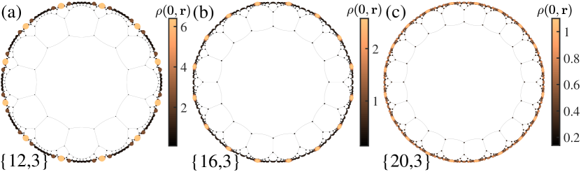
Higher-order topological phases with twelve, sixteen or twenty corner modes.—We now proceed to study the higher-order topological phase in a hyperbolic lattice respecting twelve-fold, sixteen-fold or twenty-fold rotational symmetry by constructing the Hamiltonian in hyperbolic , , or lattices. Such Hamiltonians respect chiral symmetry and the corresponding symmetry with , , or . Figure 4 illustrates the local DOS at zero energy in the Poincaré disk, indicating the existence of twelve, sixteen and twenty corner modes, respectively (see the energy spectrum in Supplemental Material S-9). All these phases arise from the allowed rotational symmetry of a hyperbolic lattice, and thus cannot exist in a crystalline material. Even in a quasicrystal, it is unclear whether sixteen-fold or twenty-fold rotational symmetry can occur, to the best of our knowledge Sunbook .
In summary, we have theoretically predicted higher-order topological phases in hyperbolic lattices with eight-fold, twelve-fold, sixteen-fold or twenty-fold rotational symmetry, which have eight, twelve, sixteen and twenty corner modes, respectively. Such phases are not allowed in a crystalline material. For the hyperbolic lattices, we identify a higher-order topological phase with a finite edge energy gap and a gapless phase. Given that hyperbolic lattices have been experimentally realized in circuit quantum electrodynamics Houck2019nat and electric circuits Zhang2022NC ; Lenggenhager2022NC ; Boettcher2022arxiv , higher-order topological phases in hyperbolic lattices may be observed in these systems. In fact, higher-order topological phases in square lattices have been observed in phononic Huber2018Nat , microwave Bahl2018Nat , electric circuit Thomale2018NP , and photonic systems Hafezi2019NP . Our work may also inspire the interest of studying higher-order topological phases in hyperbolic lattices in quantum simulators, such as cold atom systems Browaeys2016Science ; Lukin2016Science .
Acknowledgements.
We thank J.-H. Wang for helpful discussions. This work is supported by the National Natural Science Foundation of China (Grant No. 11974201) and Tsinghua University Dushi Program.References
- (1) A. J. Kollár, M. Fitzpatrick, and A. A. Houck, Nature 571, 45 (2019).
- (2) W. Zhang, H. Yuan, N. Sun, H. Sun, and X. Zhang, Nat. Commun. 13, 2937 (2022).
- (3) P. M. Lenggenhager, A. Stegmaier, L. K. Upreti, T. Hofmann, T. Helbig, A. Vollhardt, M. Greiter, C. H. Lee, S. Imhof, H. Brand, T. Kießling, I. Boettcher, T. Neupert, R. Thomale, T. Bzdušek, Nat. Commun. 13, 4373 (2022).
- (4) A. Chen, H. Brand, T. Helbig, T. Hofmann, S. Imhof, A. Fritzsche, T. Kießling, A. Stegmaier, L. K. Upreti, T. Neupert, T. Bzdušek, M. Greiter, R. Thomale, and I. Boettcher, arXiv:2205.05106 (2022).
- (5) A. J. Kollár, M. Fitzpatrick, P. Sarnak, and A. A. Houck, Commun. Math. Phys. 376, 1909 (2019).
- (6) S. Yu, X. Piao, and N. Park, Phys. Rev. Lett. 125, 053901 (2020).
- (7) I. Boettcher, P. Bienias, R. Belyansky, A. J. Kollár, and A. V. Gorshkov, Phys. Rev. A 102, 032208 (2020).
- (8) J, Maciejko and S. Rayan, Sci. Adv. 7, eabe9170 (2021).
- (9) K. Ikeda, S. Aoki, and Y. Matsuki, J. Phys.: Condens. Matter 33, 485602 (2021).
- (10) A. Saa, E. Miranda, and F. Rouxinol, arXiv:2108.08854 (2021).
- (11) J. Maciejko, S. Rayan, Proc. Natl. Acad. Sci. 119, e2116869119 (2022).
- (12) P. Bienias, I. Boettcher, R. Belyansky, A. J. Kollár, and A. V. Gorshkov, Phys. Rev. Lett. 128, 013601 (2022).
- (13) A. Stegmaier, L. K. Upreti, R. Thomale, and I. Boettcher, Phys. Rev. Lett. 128, 166402 (2022).
- (14) I. Boettcher, A. V. Gorshkov, A. J. Kollár, J. Maciejko, S. Rayan, and R. Thomale, Phys. Rev. B 105, 125118 (2022).
- (15) D. M. Urwyler, P. M. Lenggenhager, I. Boettcher, R. Thomale, T. Neupert, T. Bzdušek, arXiv:2203.07292 (2022).
- (16) Z.-R. Liu, C.-B. Hua, T. Peng, and B. Zhou, Phys. Rev. B 105, 245301 (2022).
- (17) N. Cheng, F. Serafin, J. McInerney, Z. Rocklin, K. Sun, and X. Mao, arXiv:2203.15208 (2022).
- (18) T. Bzdušek and J. Maciejko, Phys. Rev. B 106, 155146 (2022).
- (19) R. Mosseri, R. Vogeler, and J. Vidal, Phys. Rev. B 106, 155120 (2022).
- (20) W. A. Benalcazar, B. A. Bernevig, and T. L. Hughes, Science 357, 61 (2017).
- (21) M. Sitte, A. Rosch, E. Altman, and L. Fritz, Phys. Rev. Lett. 108, 126807 (2012).
- (22) F. Zhang, C. L. Kane, and E. J. Mele, Phys. Rev. Lett. 110, 046404 (2013).
- (23) R.-J. Slager, L. Rademaker, J. Zaanen, and L. Balents, Phys. Rev. B 92, 085126 (2015)
- (24) J. Langbehn, Y. Peng, L. Trifunovic, F. von Oppen, and P. W. Brouwer, Phys. Rev. Lett. 119, 246401 (2017).
- (25) Z. Song, Z. Fang, and C. Fang, Phys. Rev. Lett. 119, 246402 (2017).
- (26) F. Schindler, A. M. Cook, M. G. Vergniory, Z. Wang, S. S. P. Parkin, B. A. Bernevig, and T. Neupert, Sci. Adv. 4, eaat0346 (2018).
- (27) M. Lin and T. L. Hughes, Phys. Rev. B 98, 241103(R) (2018).
- (28) L. Trifunovic and P. W. Brouwer, Phys. Rev. X 9, 011012 (2019).
- (29) M. Rodriguez-Vega, A. Kumar, and B. Seradjeh, Phys. Rev. B 100, 085138 (2019).
- (30) D. Cǎlugǎru, V. Juričić, and B. Roy, Phys. Rev. B 99, 041301(R) (2019).
- (31) D. Varjas, A. Lau, K. Pöyhönen, A. R. Akhmerov, D. I. Pikulin, and I. C. Fulga, Phys. Rev. Lett. 123, 196401 (2019).
- (32) X.-L. Sheng, C. Chen, H. Liu, Z. Chen, Z.-M. Yu, Y. X. Zhao, and S. A. Yang, Phys. Rev. Lett. 123, 256402 (2019).
- (33) A. Agarwala, V. Juričić, and B. Roy, Phys. Rev. Research 2, 012067(R) (2020).
- (34) Y.-B. Yang, K. Li, L.-M. Duan, and Y. Xu, Phys. Rev. Research 2, 033029 (2020).
- (35) R. Chen, C.-Z. Chen, J.-H. Gao, B. Zhou, and D.-H. Xu, Phys. Rev. Lett. 124, 036803 (2020).
- (36) A. Tiwari, M.-H. Li, B. A. Bernevig, T. Neupert, and S. A. Parameswaran, Phys. Rev. Lett. 124, 046801 (2020).
- (37) Q.-B. Zeng, Y.-B. Yang, and Y. Xu, Phys. Rev. B 101, 241104(R) (2020).
- (38) C. Chen, Z. Song, J.-Z. Zhao, Z. Chen, Z.-M. Yu, X.-L. Sheng, and S. A. Yang, Phys. Rev. Lett. 125, 056402 (2020).
- (39) Y.-L. Tao, N. Dai, Y.-B. Yang, Q.-B. Zeng, and Y. Xu, New J. Phys. 22, 103058 (2020).
- (40) J.-H. Wang, Y.-B. Yang, N. Dai, and Y. Xu, Phys. Rev. Lett. 126, 206404 (2021).
- (41) See the Supplemental Material.
- (42) T.-Y. Fan, W. Yang, H. Cheng, and X.-H. Sun, Generalized Dynamics of Soft-Matter Quasicrystals: Mathematical Models, Solutions and Applications (Springer, Singapore, 2022), 2nd ed.
- (43) B. Kang, K. Shiozaki, and G. Y. Cho, Phys. Rev. B 100, 245134 (2019).
- (44) W. A. Wheeler, L. K. Wagner, and T. L. Hughes, Phys. Rev. B 100, 245135 (2019).
- (45) Y.-B. Yang, K. Li, L.-M. Duan, and Y. Xu, Phys. Rev. B 103, 085408 (2021).
- (46) C.-A. Li, B. Fu, Z.-A. Hu, J. Li, and S.-Q. Shen, Phys. Rev. Lett. 125, 166801 (2020).
- (47) In Fig. 2(a), on the right side of the vertical dashed line, there is a tiny plateau region where the energy gap in momentum space is finite. Such a region arises from the edge energy gap closing if we consider open boundaries along the direction of or .
- (48) M. Serra-Garcia, V. Peri, R. Süsstrunk, O. R. Bilal, T. Larsen, L. G. Villanueva, and S. D. Huber, Nature (London) 555, 342 (2018).
- (49) C. W. Peterson, W. A. Benalcazar, T. L. Hughe, and G. Bahl, Nature (London) 555, 346 (2018).
- (50) S. Imhof, C. Berger, F. Bayer, J. Brehm, L. W. Molenkamp, T. Kiessling, F. Schindler, C. H. Lee, M. Greiter, T. Neupert, and R. Thomale, Nat. Phys. 14, 925 (2018).
- (51) S. Mittal, V. V. Orre, G. Zhu, M. A. Gorlach, A. Poddubny, and M. Hafezi, Nat. Photonics 13, 692 (2019).
- (52) D. Barredo, S. de Léséleuc, V. Lienhard, T. Lahaye, and A. Browaeys, Science 354, 1021 (2016).
- (53) M. Endres, H. Bernien, A. Keesling, H. Levine, E. R. Anschuetz, A. Krajenbrink, C. Senko, V. Vuletić , M. Greiner, and M. D. Lukin, Science 354, 1024 (2016).
In the Supplemental Material, we will give a pedagogical introduction to how the hyperbolic lattices on the Poincaré disk are generated based on circular inversion in Section S-1, show how the modified angle is defined and present the momentum space Hamiltonian in Section S-2, prove that in Section S-3, provide more detailed discussion on the band and topological properties of the higher-order topological hyperbolic semimetal phase in the 4D momentum space in Section S-4, provide the energy spectrum and local DOS for the model with translational symmetry calculated in a geometry with open boundaries in Section S-5, utilize the corner charge to characterize the gapped topological phases in Section S-6, show that the higher-order topological phase continues to exist in a much larger system even though the mini-gap becomes very small and how the reentrant gapped phase and the branching arise in Section S-7, provide the density profile of the states in the vicinity of zero energy in the gapless phase in Section S-8, present the energy spectra of the hyperbolic {12,3}, {16,3} and {20,3} lattices with respect to the system parameter in Section S-9, and finally present the effect of weak disorder on topological phases in Section S-10.
I S-1. Generation of hyperbolic lattices based on circular inversion
In this section, we will follow Ref. HartshornebookS to give a pedagogical introduction to how the hyperbolic lattices on the Poincaré disk are generated based on circular inversion.
Hyperbolic lattices can be described by the Poincaré disk model, where points are written as . The metric on this disk is
| (S1) |
where is the curvature radius, which is equal to the radius of the disk (here we set ). According to this metric, the geodesic line between points and is the circular arc of an inversion circle.
Consider the outmost cirlce of the disk with center [see Fig. S1(a)]. We now show how to obtain another circle determined by the points , and their inverses with respect to the circle . The inverse of (marked as ) (similarly for ) lies on the ray from to satisfying
| (S2) |
These four points lie on the inversion circle with center and redius . The geodesic line between and on the disk is the circular arc of the inversion circle .
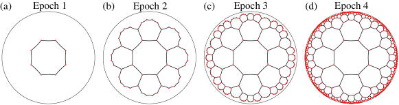
We are now in a position to present the process of constructing a hyperbolic lattice with inversion circles. First, we plot the central polygon with vertices and connect two neighboring ones through geodesic lines, which is the lattice at epoch 1 [see Fig. S2(a)]. These vertices are determined by where , is an arbitrary value, and is the distance from the center to a vertex determined by
| (S3) |
Second, we show how to generate a new polygon adjacent to an edge (e.g., ) of the first one. The vertices of this polygon are the inverses of with respect to the circle [see Fig. S1(b)]. Similarly, one can obtain the vertices adjacent to other edges, ending up with a lattice at epoch 2 [see Fig. S2(b)]. In Fig. S2(c) and (d), we also plot the hyperbolic lattices at epoch 3 and 4, respectively.
II S-2. Model with hyperbolic translational symmetry and the momentum space Hamiltonian
In this section, we will provide Fig. S3 where the modified angle is defined and show how to construct the momentum space Hamiltonian via twisted boundary conditions.
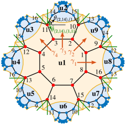
Fig. S3 displays the hyperbolic {8,3} lattice with nine unit cells . In the hopping matrix in the Hamiltonian in Eq. (4) in the main text, is the angle of the vector from the site to the site . Note that here and can be either a composite index or a single index uniquely labeling each site. For example, denotes the site 14 in the unit cell (see Fig. S3). In Eq. (4) in the main text, the hopping from the site 11 in the unit cell to the site 14 in the unit cell is determined by the angle labeled in the figure. However, this model breaks the translational symmetry. To restore the translational symmetry without breaking the symmetry, we follow Ref. Urwyler2022arxivS to modify the intercell hopping by replacing by a modified one . For example, for the hopping mentioned above, we use the modified angle , the polar angle of the direction of the generator (green line in Fig. S3). The other angles for the intercell hopping are also modified similarly (see the green lines in Fig. S3). After that, we apply the translational operations (generated by four generators ) to generate the entire Hamiltonian, which preserves both translational symmetry and symmetry.
We now provide the momentum space Bloch Hamiltonian based on the hyperbolic band theory Rayan2021sciaS ; Rayan2022PNASS ; Mao2022arxivS . The onsite and hopping term inside the first unit cell (the light orange region in Fig. S3) is
| (S4) |
The Bloch Hamiltonian is given by
| (S5) |
where
| (S6) | |||||
| (S7) | |||||
| (S8) | |||||
| (S9) |
where denotes the modified angle from the th site in the unit cell to the th site in the unit cell .
III S-3. Proof of the relation on the quadrupole moment
In this section, we will prove that , where is the average quadrupole moment defined in Eq. (2) in the main text. The system in the main text respects the symmetry, and with this symmetry, the Hamiltonian in momentum space satisfies
| (S10) |
where is a unitary matrix. Fixing parameter momenta and spanning square lattice momenta , we obtain the set of occupied eigenstates with being the th occupied eigenstate of (one of occupied states). One can obtain the column vector using the eigenstate of , that is, , where , denotes the position of the th unit cell and is an eigenstate of . For clarity, we write down the definition of the quadruple moment as
| (S11) |
where we have explicitly indicated that is a function of and .
Thanks to the symmetry, is an eigenstate of . It follows that applying (for an square lattice) to leads to , that is,
| (S12) |
where in the Hamiltonian , is replaced by and is replaced by . realizes the exchange of column vectors so as to arrange the occupied eigenstates in a certain order (in fact, the order is not important). As a result, we have
| (S13) | ||||
Clearly, commutes with the , i.e., . We thus arrive at
| (S14) | ||||
Averaging the quadrupole moment over parameter momenta , we have the following relations:
| (S15) | ||||
Similarly, one can also prove that and by choosing different pairs of parameter momenta.
IV S-4. The band and topological properties of the semimetal phase in the 4D momentum-space
In this section, we will provide more detailed discussion on the band and topological properties of the higher-order topological hyperbolic semimetal phase in the 4D momentum space. In Fig. S4(a), we plot the gap of as a function of in the 4D Brillouin zone for different system sizes. Clearly, the gap of closes when , leading to a gapless phase.
To illustrate the gapless structure in the semimetal phase, we plot the gapless region for in Fig. S4(b) with color denoting . We find eight degenerate nodes. We also display the distribution of the quadrupole moment in the plane in Fig. S4(c). We see that a part in the Brillouin zone exhibits of and the other part has zero , resulting in a fractional value of the average quadrupole moment. The degenerate nodes projected on the plane cannot completely separate topologically nontrivial and trivial regimes. This is due to the fact that a quadrupole topological insulator can undergo phase transitions through edge energy gap closing without involving any bulk energy gap closing Xu2020PPRS .
V S-5. The energy spectrum and local DOS for the model with translational symmetry
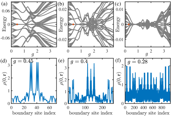
In the section, we will show the energy spectrum and local DOS for the model with translational symmetry calculated in a geometry with open boundaries. The energy spectrum in Fig. S5(a) clearly illustrates the existence of zero-energy states, which are localized in the vicinity of a corner position as reflected by the local DOS at zero energy in Fig. S5(d). We also see the existence of a gapless phase. However, for larger systems at epoch 5 and 6, we find that the energy spectrum changes dramatically for different system sizes. The consequence is that for a large system, we cannot observe a local DOS with a clear main peak on the boundary [see Fig. S5(f)]. In this case, we can hardly claim that the system is a topological phase in the thermodynamic limit.
VI S-6. Corner charge
For gapped topological phases with corner modes, boundary obstructions lead to the corner-localized fractional charges Queiroz2021PRBS ; Xu2020PPRS . In our case, such corner charges should appear over a 1/8 sector [see Fig. S6(a)]. Therefore, we use the net charge over a sector at half filling to characterize the topological feature of the system in real space, which is defined as
| (S16) |
where is the number of sites in this sector and is the th component of the th occupied eigenstate at site r. The first term arises from the background positive charge over (each site contributes a charge in units of ). To determine the part contributed by electrons, we introduce a small -term , so that the eightfold degeneracy of the zero-energy states is lifted, leading to four corner states with positive energy and the other four with negative energy. As a result, only four corner states are occupied at hall filling.
In Fig. S6(b), we plot with respect to . In the deep gapped () and reentrant gapped () regimes, approaches the quantized value of , reflecting that these two regimes are topologically nontrivial. Note that when is small, there is a small gap for the corner modes due to finite-size effects, leading to the inaccurate evaluation of the corner charge. We in fact also plot the corner charge for a larger system at epoch 5, illustrating that it is closer to in the gapped regime (see the inset in Fig. 2 in the main text). In the gapped trivial phase (), the corner charge declines to zero. Also note that in the gapless region, the corner charge is not a well defined quantity.
VII S-7. Finite-size analysis
In this section, we will first show that the higher-order topological phase continues to exist in a much larger system even though the mini-gap becomes very small and then discuss how the reentrant gapped phase and the branching arise.
VII.1 A. Energy spectra, energy gap, local DOS for larger systems
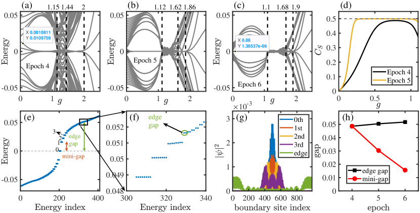
In this subsection, we will show that the higher-order topological phase may exist in the thermodynamic limit through finite-size analysis. In Fig. S7, we plot the energy spectrum for a hyperbolic {8,3} lattice at epoch 4, 5 and 6 corresponding to 768, 2888 and 10800 sites, respectively. The figure shows that the transition point from the gapped phase to the gapless one changes very slightly with the system size, suggesting its presence in the thermodynamic limit, which is very different from the hyperbolic model with translational symmetry as shown in Fig. S5. In this figure, we also see an apparent decline of the energy gap [defined as the mini-gap shown in Fig. S7(e)] as the system size increases [also see the red circles in Fig. S7(h)]. Despite the decrease of the gap, we are surprised to see that the eight-fold degeneracy of zero-energy modes becomes better. For example, at , there exists a small energy splitting of for the zero-energy states for a system at epoch 4 [Fig. S7(a)]; however, the splitting drops to about for a much larger system at epoch 6 [Fig. S7(c)]. Such a significant decline strongly suggests the existence of eight-fold degeneracy at zero energy and thus the topological phase in the thermodynamic limit. To further characterize the topology, we calculate the corner charge for different system sizes and find that it is closer to the quantized value of for a larger system compared with a smaller one [see Fig. S7(d)].
Our numerical results also show that the mini-gap states are also eight-fold degenerate [see Fig. S7(e)] and are mainly localized near a corner [see Fig. S7(g)]. In fact, we find many eight-fold degenerate states with small finite energies. Interestingly, as we increase the energy, the degeneracy suddenly drops to the double one corresponding to the states mainly localized at the center of edges [see the density profile (green line in Fig. S7(g)) of the state encircled by the green circle in Fig. S7(f)]. There, the energy spectrum becomes more continuous. We therefore call the gap determined by this energy the edge energy gap [see Fig. S7(e)-(f)]. While the mini-gap decreases with the system size, the edge energy gap remains almost unchanged for different system sizes [see Fig. S7(h)].
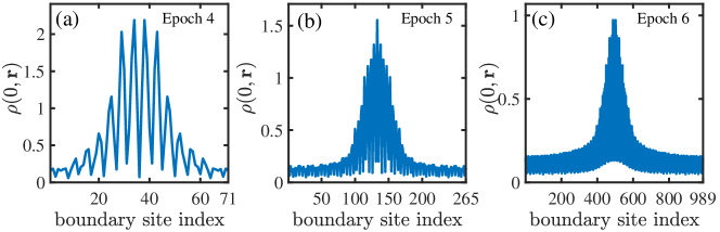
To further confirm the existence of the topological phase in the thermodynamic limit, we plot the distribution of the zero-energy local DOS on the boundary of a hyperbolic lattice at three distinct epochs. All these figures show the existence of peaks of the local DOS near the corner positions. All these results strongly suggest that the topological phase can exist in the thermodynamic limit.
VII.2 B. How do the reentrant gapped phase and the branching arise?
In the main text, we show the existence of a reentrant gapped phase. In the section, we will show that it arises from finite-size effects, which open the gap of edge states while leave the gap of corner modes unchanged.
To elaborate on the effect, we calculate the average proportion of particles on the boundary for the corner modes () and edge modes () by
| (S17) |
where is the th component of the th eigenstate at site r of the Hamiltonian in Eq. (4) in the main text under open boundary conditions, and denotes a set consisting of boundary sites of the hyperbolic lattice. is a set consisting of four eigenstates with lowest positive energy, which correspond to the corner modes in the regime with finite edge energy gap. is a set containing ten eigenstates from the fifth positive energy level to the fourteenth positive level; these modes mainly correspond to the edge modes in the regime with finite edge energy gap. denotes the number of elements in .
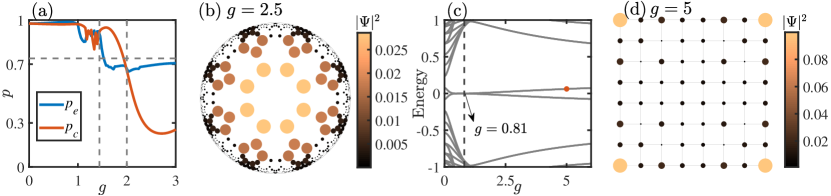
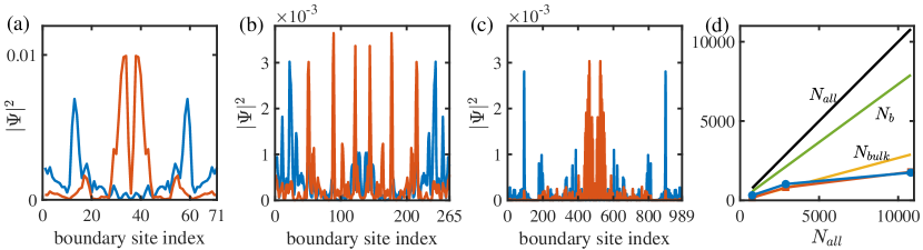
Figure S9(a) shows that as enters into the reentrant gapped regime, suddenly drops to a value smaller than , the proportion of boundary sites [ is the number of boundary sites and is the number of all sites]. It indicates that the edge states may experience some overlap due to finite-size effects so that their distribution in the bulk increases. Indeed, when we increase the system size, such overlap decreases so that the transition point from the gapless phase to the reentrant gapped one also increases, leading to a smaller reentrant regime [see Fig. S7(b) and (c)]. We thus expect that in the thermodynamic limit, the phase may disappear. The other factor accounting for the presence of the phase is that the corner modes are less sensitive to finite-size effects than the edge states, as reflected by Fig. S9(a).
However, when is further increased to , experiences a significant decline, leading to a finite gap for the corner modes. The decline is also revealed by a significant portion of the wave function permeating into the bulk [see Fig. S9(b)]. In fact, such a branching also occurs on square lattices [see the energy spectrum of the Hamiltonian in Eq. (4) in the main text on square lattice in Fig. S9(c)]. There, we also see the permeating of the wave function into the bulk.
In the square lattice case, besides the branching phase, we only see the gapped higher-order topological phase. We thus conclude that the specific geometry of hyperbolic lattices not only allows for the existence of higher-order topological phases with the symmetry without crystalline counterpart, but also the appearance of several phase transitions with respect to .
VIII S-8. Local DOS and IPR in the gapless regime
In this section, we provide the density profile of the states very close to zero energy at in the gapless phase in Fig. S10(a)-(c), showing the coexistence of states with large occupation close to a corner or the center of an edge. Interestingly, for the latter states, they have well localized property instead of an extended property. To identify the localized property, we plot the number of boundary sites and the number of bulk sites as a function of the number of all sites , as well as the inverse of the mean inverse participation ratio (IPR) in Fig. S10(d). Different from the crystalline system, in a hyperbolic lattice, does not change with respect to the epoch number due to the fact that ( is independent of ) and Gorshkov2020PRAS ; Saa2021arxivS . In the {8,3} case, , and thus the boundary sites take a large proportion. Figure S10(d) shows that the inverse of the IPR for the states near zero energy is much smaller than , implying that these states are far from uniformly distributed over the boundary sites. Such a localized property may arise from the rapid change of the angle between two sites on the boundary, which plays the role of disorder.
IX S-9. The energy spectrum for the hyperbolic {12,3}, {16,3} and {20,3} lattices
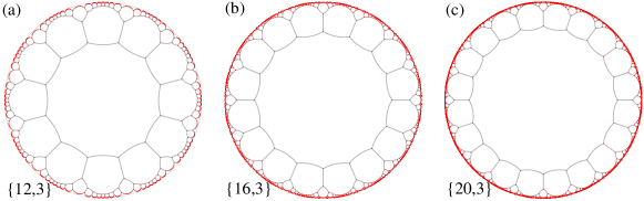
In this section, we present the energy spectra of the hyperbolic {12,3}, {16,3} and {20,3} lattices with respect to the system parameter . In Fig. S11, we display their lattice structures at epoch 2. Note that the initial setting about of the central polygon is for the hyperbolic {12,3} lattice, and for the hyperbolic {16,3} and {20,3} lattices.
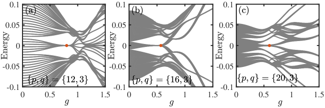
Figure S12 displays the energy spectra of the tight-binding Hamiltonian in Eq. (4) in the main text as a function of based on these lattice structures. Similar to the {8,3} case, there exists a topological region with zero-energy modes (see Fig. 4 in the main text for the local DOS at zero energy for the parameter marked out as red solid circles). In the {12,3} case, we similarly see the presence of a gapless phase. However, the {16,3} and {20,3} cases do not exhibit the presence of the gapless phase.
X S-10. Stability against disorder
In this section, we discuss the effect of weak disorder on topological phases by introducing the on-site disorder mass term for the hyperbolic {8,3} lattice in the Hamiltonian in Eq. (4) in the main text,
| (S18) |
where is a random variable that is uniformly distributed in respecting symmetry and is the strength of disorder. This term respects the chiral symmetry and symmetry, i.e., .
To illustrate that the higher-order topological hyperbolic phases are stable against weak disorder, we calculate the local DOS at zero energy averaged over samples in the presence of weak disorder with . Figure S13 shows that the existence of disorder does not destroy the corner modes, indicating the stability of these topological phases against weak disorder.
References
- (1) R. Hartshorne, Geometry: Euclid and Beyond (Springer New York, 2000).
- (2) D. M. Urwyler, P. M. Lenggenhager, I. Boettcher, R. Thomale, T. Neupert, T. Bzdušek, arXiv:2203.07292 (2022).
- (3) J, Maciejko and S. Rayan, Sci. Adv. 7, eabe9170 (2021).
- (4) J. Maciejko, S. Rayan, Proc. Natl. Acad. Sci. 119, e2116869119 (2022).
- (5) N. Cheng, F. Serafin, J. McInerney, Z. Rocklin, K. Sun, and X. Mao, arXiv:2203.15208 (2022).
- (6) Y.-B. Yang, K. Li, L.-M. Duan, and Y. Xu, Phys. Rev. Research 2, 033029 (2020).
- (7) E. Khalaf, W. A. Benalcazar, T. L. Hughes, and R. Queiroz, Phys. Rev. Research 3, 013239 (2021).
- (8) I. Boettcher, P. Bienias, R. Belyansky, A. J. Kollár, and A. V. Gorshkov, Phys. Rev. A 102, 032208 (2020).
- (9) A. Saa, E. Miranda, and F. Rouxinol, arXiv:2108.08854 (2021).