Higher order time discretization method for a class of semilinear stochastic partial differential equations with multiplicative noise

Yukun Li Department of Mathematics, University of Central Florida, Orlando, FL, 32816, U.S.A. ([email protected]). This author was partially supported by the NSF grant DMS-2110728. Liet Vo Department of Mathematics, Statistics and Computer Science, The University of Illinois at Chicago, Chicago, IL 60607, U.S.A. ([email protected]). Guanqian Wang Department of Mathematics, University of Central Florida, Orlando, FL, 32816, U.S.A. ([email protected]). This author was partially supported by the NSF grant DMS-2110728.

Abstract

In this paper, we consider a new approach for semi-discretization in time and spatial discretization of a class of semi-linear stochastic partial differential equations (SPDEs) with multiplicative noise. The drift term of the SPDEs is only assumed to satisfy a one-sided Lipschitz condition and the diffusion term is assumed to be globally Lipschitz continuous. Our new strategy for time discretization is based on the Milstein method from stochastic differential equations. We use the energy method for its error analysis and show a strong convergence order of nearly $1$ for the approximate solution. The proof is based on new Hölder continuity estimates of the SPDE solution and the nonlinear term. For the general polynomial-type drift term, there are difficulties in deriving even the stability of the numerical solutions. We propose an interpolation-based finite element method for spatial discretization to overcome the difficulties. Then we obtain $H^{1}$ stability, higher moment $H^{1}$ stability, $L^{2}$ stability, and higher moment $L^{2}$ stability results using numerical and stochastic techniques. The nearly optimal convergence orders in time and space are hence obtained by coupling all previous results. Numerical experiments are presented to implement the proposed numerical scheme and to validate the theoretical results.

keywords:

Stochastic partial differential equations, multiplicative noise, Wiener process, Itô stochastic integral, Milstein scheme, finite element method, error estimates.

AMS:

65N12, 65N15, 65N30

1 Introduction

We consider the following initial-boundary value problem for general semi-linear stochastic partial differential equations (SPDEs) with function-type multiplicative noise:

(1.1)	$\displaystyle du$	$\displaystyle=\bigl{[}\Delta u+F(u)\bigr{]}\,dt+G(u)\,dW(t)$	$\displaystyle\qquad\mbox{a.s. in}\,(0,T)\times D,$
(1.2)	$\displaystyle u$	$\displaystyle=0$	$\displaystyle\qquad\mbox{a.s. on }(0,T)\times\partial D,$
(1.3)	$\displaystyle u(0)$	$\displaystyle=u_{0}$	$\displaystyle\qquad\mbox{a.s. in}\,D,$

where $D=(0,L)^{d}\subset\mathbb{R}^{d}\,(d=1,2)$ . $F,G$ are two given functions that will be specified later. $\{W(t);t\geq 0\}$ denotes an ${{\mathbb{R}}}$ -valued Wiener process.

The corresponding stochastic ordinary differential equations of (1.1) (without the Laplacian term) are studied in [17, 23] for the case when both $F$ and $G$ are Lipschitz continuous, and in [14] for the case when $G$ satisfies the one-sided Lipschitz condition as stated in (2.7). The strong and weak divergence is considered in [15] for some $F$ which are not Lipschitz continuous. Besides, the corresponding stochastic partial differential equations of (1.1) when $F$ is Lipschitz and non-Lipschitz continuous and when $G$ is additive and multiplicative are studied in [8, 9, 10, 21, 22] based on the variational approach and in [4, 12, 13, 16, 18, 19, 20] based on the semigroup approach. Here the half-order convergence is established in [22] when the drift term is $F(u)=u-u^{3}$ using the Euler-type scheme. The half-order convergence is established in [10] for the drift term in (2.6) and diffusion term in assumptions (A1)–(A3) for a fully discrete scheme.

The primary goal of this paper is to design and analyze a first-order numerical scheme for the time discretization of the problem (1.1)–(1.3). Specifically, we design a new time discretization method first and then propose an interpolation finite element method, which is based on the new time scheme to discretize the space. Our idea for the time discretization method is inspired by the Milstein method [24] from stochastic differential equations and the semi-discrete in time strategy of the stochastic Stokes equations in [28]. In addition, the diffusion function $G$ is assumed to satisfy the global Lipschitz condition while the drift-nonlinear function $F$ is only one-sided Lipschitz. Furthermore, to establish the rates of convergence of the proposed scheme, we use the energy method followed by two steps: the first step is to prove the first-order error order in time by utilizing several established Hölder continuity estimates. The second step is to prove the optimal error order in space. To achieve this, the $H^{1}$ stability of the numerical solution is needed. The $H^{1}$ -seminorm stability of the numerical solution is proved first and based on which the $L^{2}$ stability of the numerical solution is established.

The remainder of this paper is organized as follows. In Section 2, several Hölder continuity results about the strong solution are proved. These results will be used in establishing the semi-discrete in-time error estimates. In Section 3, we present the new approach for the time discretization and its a priori stability as well as the error estimates of the semi-discrete solution are proved. The convergence order is proved to be nearly $1$ for the proposed scheme in $L^{2}$ -norm and the energy norm. In Section 4, we consider an interpolation finite element method for spatial discretization. The finite element method is designed where the interpolation operator is utilized to overcome the difficulty resulting from nonlinearity. Through this approach, the second moment and higher moment $H^{1}$ stability results are proved first, based on which the second moment and higher moment $L^{2}$ stability results are proved. Finally, the error estimates with optimal convergence order in space are established based on those stability results. In Section 5, several numerical tests including different initial conditions, drift terms, and diffusion terms are used to validate the theoretical results.

2 Preliminaries

Let $\mathcal{T}_{h}$ be the triangulation of $\mathcal{D}$ satisfying the following assumption [30]:

(2.1)

\frac{1}{d(d-1)}\sum_{K\supset E}|\kappa_{E}^{K}|\cot\theta_{E}^{K}\geq 0,

where $E$ denotes the edge of simplex $K$ . Note this assumption is just the Delaunay triangulation when $d=2$ . In 3D, the notations in the assumption (2.1) are as follows: $a_{i}\ (1\leq i\leq d+1)$ denote the vertices of $K$ , $E=E_{ij}$ the edge connecting two vertices $a_{i}$ and $a_{j}$ , $F_{i}$ the $(d-1)$ -dimensional simplex opposite to the vertex $a_{i}$ , $\theta_{ij}^{K}$ or $\theta_{E}^{K}$ the angle between the faces $F_{i}$ and $F_{j}$ , and $\kappa_{E}^{K}=F_{i}\cap F_{j}$ .

Let ${\mathcal{H}}$ , ${\mathcal{K}}$ be two Hilbert spaces. Then, $\mathcal{L}({\mathcal{H}},{\mathcal{K}})$ is the space of linear maps from ${\mathcal{H}}$ to ${\mathcal{K}}$ . For $m\in\mathbb{N}$ , inductively define

(2.2)

\displaystyle\mathcal{L}_{m}({\mathcal{H}},{\mathcal{K}}):=\mathcal{L}({\mathcal{H}},\mathcal{L}_{m-1}({\mathcal{H}},{\mathcal{K}})),

as the space of all multi-linear maps from ${\mathcal{H}}\times\cdots\times{\mathcal{H}}$ ( $m$ times) to ${\mathcal{K}}$ for $m\geq 2$ .

For some function $G:{\mathcal{H}}\rightarrow{\mathcal{K}}$ , we define the Gateaux derivative of $G$ with respect to $u\in{\mathcal{H}}$ , $DG(u)\in\mathcal{L}({\mathcal{H}},{\mathcal{K}})$ , whose action is seen as

\displaystyle v\mapsto DG(u)(v)\qquad\forall v\in{\mathcal{H}}.

In general, we denote $D^{k}G(u)\in\mathcal{L}_{m}({\mathcal{H}},{\mathcal{K}})$ , as the $k$ -Gateaux derivative of $G$ with respect to $u\in{\mathcal{H}}$ .

Below, we state the assumptions on the functionals $G,F:{\mathcal{H}}\rightarrow{\mathcal{K}}$ .

(A1)

$G$ is globally Lipschitz continuous and has linear growth. Namely, there exists a constant $C>0$ such that for all ${v},{w}\in{\mathcal{H}}$


(2.3a)	$\displaystyle\\|G({v})-G({w})\\|_{{\mathcal{K}}}$	$\displaystyle\leq C\\|{v}-{w}\\|_{{\mathcal{H}}}\,,$
(2.3b)	$\displaystyle\\|G({v})\\|_{{\mathcal{K}}}$	$\displaystyle\leq C\bigl{(}\\|{v}\\|_{{\mathcal{H}}}+1\bigr{)}\,.$

(A2)

There exists a constant $C>0$ such that

(2.4)

\displaystyle\|DG\|_{L^{\infty}({\mathcal{H}};\mathcal{L}({\mathcal{H}},{\mathcal{K}}))}+\|D^{2}G\|_{L^{\infty}({\mathcal{H}};\mathcal{L}_{2}({\mathcal{H}},{\mathcal{K}}))}\leq C.

(A3)

There exists a constant $C>0$ such that for all $u,v\in\mathcal{H}$

(2.5) $\displaystyle\|(DG(u)-DG(v)){G}(v)\|_{\mathcal{K}}\leq C\|u-v\|_{\mathcal{H}}.$

In this paper, suppose that $G:H^{1}_{0}(D)\rightarrow H^{1}_{0}(D)$ , and

(2.6)

\displaystyle F(u)=c_{0}u-c_{1}u^{3}-c_{2}u^{5}-c_{3}u^{7}-\cdots,

where $c_{i}\geq 0,i=0,1,2,\cdots$ . For simplicity, we choose $F(u)=u-u^{q}$ for all odd numbers $q\geq 3$ . Then $F$ satisfies the following one-sided Lipschitz condition [25]

(2.7)

\displaystyle\langle a-b,F(a)-F(b)\rangle\leq\mu|a-b|^{2}\qquad\forall a,b\in\mathbb{R}^{d},

where $\mu$ is a positive constant.

Under the above assumptions for the drift term and the diffusion term, it can be proved in [11] that there exists a unique strong variational solution u such that

(2.8)		$\displaystyle\bigl{(}u(t),\phi\bigr{)}$	$\displaystyle=\bigl{(}u(0),\phi\bigr{)}-\int_{0}^{t}\bigl{(}\nabla u(s),\nabla\phi\bigr{)}\,ds$
		$\displaystyle+\int_{0}^{t}\bigl{(}F(u(s)),\phi\bigr{)}\,ds+\int_{0}^{t}\bigl{(}G(u(s)),\phi\bigr{)}\,dW(s)\quad\forall\phi\in H_{0}^{1}(D)$

holds $\mathbb{P}$ -almost surely. Moreover, when the initial condition $u_{0}$ is sufficiently smooth, the following stability estimate for the strong solution $u$ holds

(2.9)

\displaystyle\sup_{t\in[0,T]}\mathbb{E}\bigl{[}\|u(t)\|^{2}_{H^{2}}\bigr{]}+\sup_{t\in[0,T]}\mathbb{E}\bigl{[}\|u(t)\|^{4q-2}_{L^{4q-2}}\bigr{]}\leq C,

where $q$ is the exponent in the drift term of $F(u)=u-u^{q}$ .

Next, we introduce the Hölder continuity estimates for the variational solution $u$ .

Lemma 1.

Suppose that the solution $u$ of (2.8) satisfies (2.9). For $\epsilon>0$ , let $\theta_{1}=\frac{1}{2}-\epsilon>0$ , $\theta_{2}=1-\epsilon>0$ . There exists a constant $C\equiv C(D,T,q,u_{0})>0$ , such that for all $s,t\in[0,T]$ ,

(i)

$\displaystyle{\mathbb{E}}\bigl{[}\|{u}(t)-{u}(s)\|^{2}_{H^{1}}\bigr{]}\leq C|t-s|^{2\theta_{1}}.$
(ii)

$\displaystyle{\mathbb{E}}\Bigl{[}\Bigl{\|}{u}(t)-{u}(s)-\int_{s}^{t}G(u(\xi))\,dW(\xi)\Bigr{\|}^{q}_{H^{1}}\Bigr{]}\leq C|t-s|^{q\theta_{2}},$ where $q=2,4.$
(iii)

$\displaystyle{\mathbb{E}}\bigl{[}\|{u}(t)-{u}(s)\|^{q}_{L^{q}}\bigr{]}\leq C|t-s|^{q\theta_{1}},$ where $q\geq 2$ are integers.
(iv)

$\displaystyle{\mathbb{E}}\Bigl{[}\Bigl{\|}F({u}(t))-F({u}(s))-\int_{s}^{t}DF(u(s))G(u(\xi))\,dW(\xi)\Bigr{\|}^{2}_{L^{2}}\Bigr{]}\leq C|t-s|^{2\theta_{2}}.$

Proof.

The proof of $(i)$ can be found in [10, Lemma 2.1], while the establishment of $(iii)$ is based on the semigroup theory, which can be found in many references such as [27, 26, 29]. In addition, the proof of $(ii)$ is followed [26, Lemma 10.27] and [28, Lemma 2.3] with minor modifications for $q=4$ . We just need to prove $(iv)$ . To prove $(iv)$ , we use the Taylor expansion for $F$ with respect to $u(s)\in L^{2}(D)$ as follows.

(2.10)

\displaystyle F(u(t))=F(u(s))+DF(u(s))\bigl{(}u(t)-u(s)\bigr{)}+R_{2},

where $\displaystyle R_{2}=\int_{0}^{1}(1-\eta)\bigl{(}D^{2}F(u(s)+\eta(u(t)-u(s)))\bigr{)}(u(t)-u(s))^{2}\,d\eta$ .

Therefore, we have

	$\displaystyle F(u(t))-F(u(s))-\int_{s}^{t}DF(u(s))G(u(\xi))\,dW(\xi)$
	$\displaystyle=DF(u(s))\bigg{[}u(t)-u(s)-\int_{s}^{t}G(u(\xi))\,dW(\xi)\bigg{]}+R_{2}.$

Since we have $DF(u)=1-qu^{q-1}$ , then we obtain

(2.11)		$\displaystyle\Bigl{\\|}DF(u(s))\Bigl{[}u(t)-u(s)-\int_{s}^{t}G(u(\xi))\,dW(\xi)\Bigr{]}\Bigr{\\|}^{2}_{L^{2}}$
	$\displaystyle=\int_{D}\Bigl{\|}(1-qu(s)^{q-1})\Bigl{[}u(t)-u(s)-\int_{s}^{t}G(u(\xi))\,dW(\xi)\Bigr{]}\Bigr{\|}^{2}\,dx$
	$\displaystyle\leq\int_{D}2(1+q^{2}\|u(s)\|^{2(q-1)})\Bigl{\|}\Bigl{[}u(t)-u(s)-\int_{s}^{t}G(u(\xi))\,dW(\xi)\Bigr{]}\Bigr{\|}^{2}\,dx$
	$\displaystyle\leq 2\Bigl{(}\int_{D}(1+q^{2}\|u(s)\|^{2(q-1)})^{2}\,dx\Bigr{)}^{\frac{1}{2}}\Bigl{\\|}u(t)-u(s)-\int_{s}^{t}G(u(\xi))\,dW(\xi)\Bigr{\\|}^{2}_{L^{4}}$
	$\displaystyle\leq 2\Bigl{(}\int_{D}2(1+q^{4}\|u(s)\|^{4(q-1)})\,dx\Bigr{)}^{\frac{1}{2}}\Bigl{\\|}u(t)-u(s)-\int_{s}^{t}G(u(\xi))\,dW(\xi)\Bigr{\\|}^{2}_{L^{4}}.$

Taking the expectation $\mathbb{E}[\cdot]$ to (2.11) and then using the Cauchy-Schwarz inequality, we obtain

(2.12)		$\displaystyle\mathbb{E}\Bigl{[}\Bigl{\\|}DF(u(s))\Bigl{[}u(t)-u(s)-\int_{s}^{t}G(u(\xi))\,dW(\xi)\Bigr{]}\Bigr{\\|}^{2}_{L^{2}}\Bigr{]}$
	$\displaystyle\leq\mathbb{E}\Bigl{[}2\Bigl{(}\int_{D}2(1+q^{4}\|u(s)\|^{4(q-1)})\,dx\Bigr{)}^{\frac{1}{2}}\Bigl{\\|}u(t)-u(s)-\int_{s}^{t}G(u(\xi))\,dW(\xi)\Bigr{\\|}^{2}_{L^{4}}\Bigr{]}$
	$\displaystyle\leq C_{q}\Bigl{(}\mathbb{E}\Bigl{[}\\|u(s)\\|^{4(q-1)}_{L^{4(q-1)}}\Bigr{]}\Bigr{)}^{\frac{1}{2}}\Bigl{(}\mathbb{E}\Bigl{[}\Bigl{\\|}u(t)-u(s)-\int_{s}^{t}G(u(\xi))\,dW(\xi)\Bigr{\\|}^{4}_{L^{4}}\Bigr{]}\Bigr{)}^{\frac{1}{2}}.$

Using the interpolation inequality that $\mathbb{E}[\|u\|^{4}_{L^{4}}]\leq C\mathbb{E}[\|u\|^{2}_{L^{2}}\|\nabla u\|^{2}_{L^{2}}]\leq C\mathbb{E}[\|u\|^{4}_{H^{1}}]$ and Lemma 1 $(iii)$ yield to

(2.13)		$\displaystyle\mathbb{E}\Bigl{[}\Bigl{\\|}u(t)-u(s)-\int_{s}^{t}G(u(\xi))\,dW(\xi)\Bigr{\\|}^{4}_{L^{4}}\Bigr{]}$
	$\displaystyle\leq C\mathbb{E}\Bigl{[}\Bigl{\\|}u(t)-u(s)-\int_{s}^{t}G(u(\xi))\,dW(\xi)\Bigr{\\|}^{4}_{H^{1}}\Bigr{]}\leq C\|t-s\|^{4\theta_{2}}.$

By using (2.9), we arrive at

(2.14)

\displaystyle\mathbb{E}\Bigl{[}\Bigl{\|}DF(u(s))\Bigl{[}u(t)-u(s)-\int_{s}^{t}G(u(\xi))\,dW(\xi)\Bigr{]}\Bigr{\|}^{2}_{L^{2}}\Bigr{]}\leq C|t-s|^{2\theta_{2}},

where $C=C_{q}\Bigl{(}\sup_{s\in[0,T]}\mathbb{E}\Bigl{[}\|u(s)\|^{4(q-1)}_{L^{4(q-1)}}\Bigr{]}\Bigr{)}^{\frac{1}{2}}$ .

It is remaining to estimate $R_{2}$ . To do that, we notice that $D^{2}F(u)=-q(q-1)u^{q-2}$ . In the end, we have

(2.15)			$\displaystyle\\|R_{2}\\|^{2}_{L^{2}}$
	$\displaystyle\leq$	$\displaystyle\int_{D}\Bigl{\|}\int_{0}^{1}(1-\eta)q(1-q)(u(s)+\eta(u(t)-u(s)))^{q-2}(u(t)-u(s))^{2}\,d\eta\Bigr{\|}^{2}\,dx$
	$\displaystyle\leq$	$\displaystyle\int_{D}\Bigl{(}q(q-1)2^{q-2}\bigl{(}\|u(s)\|^{q-2}+\|u(t)-u(s)\|^{q-2}\bigr{)}\Bigr{)}^{2}\|u(t)-u(s)\|^{4}\,dx$
	$\displaystyle\leq$	$\displaystyle\int_{D}q^{2}(q-1)^{2}2^{2q-3}\bigl{(}\|u(s)\|^{2(q-2)}+\|u(t)-u(s)\|^{2(q-2)}\bigr{)}\|u(t)-u(s)\|^{4}\,dx$
	$\displaystyle=$	$\displaystyle C_{q}\int_{D}\|u(s)\|^{2(q-2)}\|u(t)-u(s)\|^{4}\,dx+C_{q}\int_{D}\|u(t)-u(s)\|^{2q}\,dx$
	$\displaystyle\leq$	$\displaystyle C_{q}\\|u(s)\\|^{2(q-2)}_{L^{4(q-2)}}\\|u(t)-u(s)\\|^{4}_{L^{8}}+C_{q}\\|u(t)-u(s)\\|^{2q}_{L^{2q}}.$

Taking the expectation $\mathbb{E}[\cdot]$ to (2.15), using Lemma 1 $(iii)$ and then (2.9) , we obtain

(2.16)	$\displaystyle\mathbb{E}[\\|R_{2}\\|^{2}_{L^{2}}]$	$\displaystyle\leq C_{q}\mathbb{E}\bigl{[}\\|u(s)\\|^{2(q-2)}_{L^{4(q-2)}}\\|u(t)-u(s)\\|^{4}_{L^{8}}\bigr{]}+C_{q}\mathbb{E}\bigl{[}\\|u(t)-u(s)\\|^{2q}_{L^{2q}}\bigr{]}$
	$\displaystyle\leq C_{q}\Bigl{(}\mathbb{E}\bigl{[}\\|u(s)\\|^{4(q-2)}_{L^{4(q-2)}}\bigr{]}\Bigr{)}^{\frac{1}{2}}\Bigl{(}\mathbb{E}\bigl{[}\\|u(t)-u(s)\\|^{8}_{L^{8}}\bigr{]}\Bigr{)}^{\frac{1}{2}}$
	$\displaystyle\qquad\qquad+\mathbb{E}\bigl{[}\\|u(t)-u(s)\\|^{2q}_{L^{2q}}\bigr{]}$
	$\displaystyle\leq C(\|t-s\|^{4\theta_{1}}+\|t-s\|^{2q\theta_{1}})\leq C\|t-s\|^{4\theta_{1}},$

where $C=C_{q}\Bigl{(}\sup_{s\in[0,T]}\mathbb{E}\bigl{[}\|u(s)\|^{4(q-2)}_{L^{4(q-2)}}\bigr{]}\Bigr{)}^{\frac{1}{2}}$ .

The proof is complete by combining (2.14) and (2.16). ∎

3 Semi-discretization in time

In this section, we follow the strategy of the Milstein scheme in SDEs to propose a new time discretization method of (1.1). This approach generates a convergence order of nearly $1$ for the approximate solution.

3.1 Formulation of the proposed method

Let $t_{0}<t_{1}<\cdots<t_{N}$ be a uniform mesh of the interval $[0,T]$ with the time step size $\tau=\frac{T}{N}$ . Note that $t_{0}=0$ and $t_{N}=T$ .

Algorithm 1

Let $u^{0}=u_{0}$ be a given $H^{1}_{0}$ -valued random variable. Find $u^{n+1}\in H^{1}_{0}(D)$ recursively such that $\mathbb{P}$ -a.s.

(3.1)		$\displaystyle\bigl{(}u^{n+1}-u^{n},\phi\bigr{)}+\tau\bigl{(}\nabla u^{n+1},\nabla\phi\bigr{)}$	$\displaystyle=\tau\bigl{(}F(u^{n+1}),\phi\bigr{)}+\bigl{(}G(u^{n})\Delta W_{n}$
		$\displaystyle\qquad+\frac{1}{2}DG(u^{n})\,G(u^{n})\bigl{[}(\Delta W_{n})^{2}-\tau\bigr{]},\phi\bigr{)},$

for all $\phi\in H^{1}_{0}(D)$ and $\Delta W_{n}=W(t_{n+1})-W(t_{n})\sim\mathcal{N}(0,\tau)$ .

Remark 3.1.

The scheme (3.1) will produce a convergence of order nearly $1$ . The difference between (3.1) and the standard Euler-Maruyama method is the discretization of the noise term. While the Euler-type schemes, which establish a convergence order of $\frac{1}{2}$ , contain only the term $G(u^{n})\Delta W_{n}$ , the scheme (3.1) adds the extra term $\frac{1}{2}DG(u^{n})\,G(u^{n})\bigl{[}(\Delta W_{n})^{2}-\tau]$ , which is the key point to obtain a higher convergence order.

Next, we define $\displaystyle\mathcal{G}:\mathbb{R}^{+}\times H_{0}^{1}(D)\rightarrow L^{2}(D)$ by

(3.2)

\displaystyle\mathcal{G}(s;u):={G}(u)+DG(u)G(u)\,\int_{t_{n}}^{s}\,dW(r),\qquad t_{n}\leq s\leq t_{n+1}.

Then we have

	$\displaystyle\int_{t_{n}}^{t_{n+1}}\mathcal{G}(s;u^{n})\,dW(s)$	$\displaystyle=G(u^{n})\Delta W_{n}+DG(u^{n})G(u^{n})\int_{t_{n}}^{t_{n+1}}\int_{t_{n}}^{s}dW(r)\,dW(s)$
		$\displaystyle=G(u^{n})\Delta W_{n}+\frac{1}{2}DG(u^{n})G(u^{n})\bigl{[}(\Delta W_{n})^{2}-\tau\bigr{]}.$

Therefore, we rewrite (3.1) as follow:

(3.3)		$\displaystyle\bigl{(}u^{n+1}-u^{n},\phi\bigr{)}+\tau\bigl{(}\nabla u^{n+1},\nabla\phi\bigr{)}=$	$\displaystyle\tau\bigl{(}F(u^{n+1}),\phi\bigr{)}$
		$\displaystyle+\int_{t_{n}}^{t_{n+1}}\bigl{(}\mathcal{G}(s;u^{n}),\phi\bigr{)}\,dW(s).$

Next, we state the following technical lemma that is used to prove the error estimate results of this paper.

Lemma 2.

Suppose that $G$ satisfies the assumptions ${\bf(A1),(A2),(A3)}$ . Let $u_{0}\in L^{2}(\Omega;H^{1}_{0}(D)\cap H^{2}(D))$ , there exist constants $C>0$ such that the function $\mathcal{G}$ defined in (3.2) satisfies

(i)

$\displaystyle\|\mathcal{G}(s;u)-\mathcal{G}(s;v)\|_{L^{2}}\leq C\|u-v\|_{L^{2}},\qquad\forall s>0,u,v\in L^{2}(D)$ ,
(ii)

$\displaystyle\mathbb{E}\bigl{[}\bigl{\|}G(u(s))-\mathcal{G}(s;u(t_{n}))\bigr{\|}^{2}_{L^{2}}\bigr{]}\leq C|s-t_{n}|^{2(1-\epsilon)}$ , for $t_{n}\leq s<t_{n+1}$ and $\epsilon>0$ .

Proof.

The Lipschitz continuity of $\mathcal{G}$ in $(i)$ is directly obtained from the assumptions of $G$ while the proof of $(ii)$ can be found in [26, Lemma 10.36] with similar arguments.

∎

Next, we will provide the stability estimates of Algorithm 1 in the following lemma. These stability estimates will be used for the proof of the error estimates of the finite element approximation later.

Lemma 3.

Let $\{u^{n}\}$ be the solution of Algorithm 1. Then , there exists a constant $C\equiv C(D,T,u_{0},p)$ such that

(i)

$\displaystyle\sup_{1\leq n\leq N}\mathbb{E}\bigl{[}\|\nabla u^{n}\|^{2^{r}}_{L^{2}}\bigr{]}+\mathbb{E}\Bigl{[}\tau\sum_{n=1}^{N}\|\nabla u^{n}\|^{2^{r}-2}_{L^{2}}\|\Delta u^{n}\|^{2}_{L^{2}}\Bigr{]}\leq C$ , for any integers $r\geq 1$ .
(ii)

$\displaystyle\sup_{1\leq n\leq N}\mathbb{E}\bigl{[}\|\nabla u^{n}\|^{p}_{L^{2}}\bigr{]}\leq C$ , for any integers $p\geq 2$ .

Proof.

We just provide the proof of (i) when $r=1$ . When $r\geq 2$ , the proof is similar to [6, Lemma 3.1] with minor modifications. So, we skip it to save space.

To begin, we rewrite (3.1) in the strong form as follow:

(3.4)		$\displaystyle u^{n+1}-u^{n}-\tau\Delta u^{n+1}$	$\displaystyle=\tau F(u^{n+1})+G(u^{n})\Delta W_{n}$
		$\displaystyle\qquad+\frac{1}{2}DG(u^{n})G(u^{n})[(\Delta W_{n})^{2}-\tau].$

Testing the equation (3.4) by $-\Delta u^{n+1}$ and then using integration by parts we obtain

(3.5)		$\displaystyle\bigl{(}\nabla(u^{n+1}-u^{n}),\nabla u^{n+1}\bigr{)}+\tau\\|\Delta u^{n+1}\\|^{2}_{L^{2}}$
	$\displaystyle\qquad=-\tau\bigl{(}F(u^{n+1}),\Delta u^{n+1}\bigr{)}-\bigl{(}G(u^{n}),\Delta u^{n+1}\bigr{)}\Delta W_{n}$
	$\displaystyle\qquad\quad-\frac{1}{2}\bigl{(}DG(u^{n})G(u^{n}),\Delta u^{n+1}\bigr{)}\bigl{[}(\Delta W_{n})^{2}-\tau\bigr{]}$
	$\displaystyle\qquad:={\tt I+II+III}.$

By using the integration by parts, we obtain

(3.6)	$\displaystyle{\tt I}$	$\displaystyle=-\tau\bigl{(}u^{n+1},\Delta u^{n+1}\bigr{)}+\tau\bigl{(}(u^{n+1})^{q},\Delta u^{n+1}\bigr{)}$
	$\displaystyle=\tau\\|\nabla u^{n+1}\\|^{2}_{L^{2}}-\tau q\bigl{(}(u^{n+1})^{q-1}\nabla u^{n+1},\nabla u^{n+1}\bigr{)}$
	$\displaystyle=\tau\\|\nabla u^{n+1}\\|^{2}_{L^{2}}-\tau q\int_{D}(u^{n+1})^{q-1}\|\nabla u^{n+1}\|^{2}\,dx\leq\tau\\|\nabla u^{n+1}\\|^{2}_{L^{2}},$

where the last inequality of (3.6) is obtained by using the fact that, for all odd $q\geq 3$ , $\int_{D}(u^{n+1})^{q-1}|\nabla u^{n+1}|^{2}\,dx\geq 0$ .

To bound II, we take the expectation and then use the fact that $\mathbb{E}[\Delta W_{n}]=0$ . Namely,

(3.7)	$\displaystyle\mathbb{E}[{\tt II}]$	$\displaystyle=-\mathbb{E}\bigl{[}\bigl{(}G(u^{n}),\Delta(u^{n+1}-u^{n})\bigr{)}\Delta W_{n}\bigr{]}-\mathbb{E}\bigl{[}\bigl{(}G(u^{n}),\Delta u^{n}\bigr{)}\Delta W_{n}\bigr{]}$
	$\displaystyle=\mathbb{E}\bigl{[}\bigl{(}\nabla G(u^{n}),\nabla(u^{n+1}-u^{n})\bigr{)}\Delta W_{n}\bigr{]}$
	$\displaystyle\leq C\mathbb{E}[\\|\nabla u^{n}\\|^{2}_{L^{2}}\|\Delta W_{n}\|^{2}]+\frac{1}{4}\mathbb{E}\bigl{[}\\|\nabla(u^{n+1}-u^{n})\\|^{2}_{L^{2}}\bigr{]}$
	$\displaystyle=C\tau\mathbb{E}[\\|\nabla u^{n}\\|^{2}_{L^{2}}\|]+\frac{1}{4}\mathbb{E}\bigl{[}\\|\nabla(u^{n+1}-u^{n})\\|^{2}_{L^{2}}\bigr{]}.$

In addition, by using the Cauchy-Schwarz and the assumptions ${\bf(A1),(A2)}$ , we have

(3.8)	$\displaystyle\mathbb{E}[{\tt III}]$	$\displaystyle\leq\frac{C}{\tau}\mathbb{E}\bigl{[}\\|DG(u^{n})G(u^{n})\\|^{2}_{L^{2}}\|(\Delta W_{n})^{2}-\tau\|^{2}\bigr{]}+\frac{\tau}{4}\mathbb{E}\bigl{[}\\|\Delta u^{n+1}\\|^{2}_{L^{2}}\bigr{]}$
	$\displaystyle\leq\frac{C}{\tau}\mathbb{E}\bigl{[}\\|G(u^{n})\\|^{2}_{L^{2}}\|(\Delta W_{n})^{2}-\tau\|^{2}\bigr{]}+\frac{\tau}{4}\mathbb{E}\bigl{[}\\|\Delta u^{n+1}\\|^{2}_{L^{2}}\bigr{]}$
	$\displaystyle\leq C\tau\mathbb{E}\bigl{[}\\|\nabla u^{n}\\|^{2}_{L^{2}}\bigr{]}+\frac{\tau}{4}\mathbb{E}\bigl{[}\\|\Delta u^{n+1}\\|^{2}_{L^{2}}\bigr{]},$

where the last inequality of (3.8) is obtained by using the fact that $\mathbb{E}[|(\Delta W_{n})^{2}-\tau|^{2}]\leq C\tau^{2}$ .

Substituting all the estimates from ${\tt I,II,III}$ into (3.4) and absorbing the like-terms from the right side to the left side, we obtain

(3.9)		$\displaystyle\frac{1}{2}\mathbb{E}\bigl{[}\\|\nabla u^{n+1}\\|^{2}_{L^{2}}$	$\displaystyle-\\|\nabla u^{n}\\|^{2}_{L^{2}}\bigr{]}+\frac{1}{4}\mathbb{E}\bigl{[}\\|\nabla(u^{n+1}-u^{n})\\|^{2}_{L^{2}}\bigr{]}+\frac{\tau}{2}\mathbb{E}\bigl{[}\\|\Delta u^{n+1}\\|^{2}_{L^{2}}\bigr{]}$
		$\displaystyle\leq C\tau\mathbb{E}\bigl{[}\\|u^{n+1}-u^{n}\\|^{2}_{L^{2}}\bigr{]}+C\tau\mathbb{E}\bigl{[}\\|\nabla u^{n}\\|^{2}_{L^{2}}\bigr{]}.$

Next, applying the summation $\sum_{n=0}^{\ell}$ , for any $0\leq\ell<N$ , we obtain

(3.10)		$\displaystyle\mathbb{E}\bigl{[}\\|\nabla u^{\ell+1}\\|^{2}_{L^{2}}\bigr{]}+\sum_{n=0}^{\ell}\mathbb{E}\bigl{[}\\|\nabla(u^{n+1}-u^{n})\\|^{2}_{L^{2}}\bigr{]}+\tau\sum_{n=0}^{\ell}\mathbb{E}\bigl{[}\\|\Delta u^{n+1}\\|^{2}_{L^{2}}\bigr{]}$
	$\displaystyle\leq C\tau\sum_{n=0}^{\ell}\mathbb{E}\bigl{[}\\|\nabla u^{n}\\|^{2}_{L^{2}}\bigr{]}+\mathbb{E}\bigl{[}\\|\nabla u_{0}\\|^{2}_{L^{2}}\bigr{]}+C\tau\sum_{n=0}^{\ell}\mathbb{E}\bigl{[}\\|u^{n+1}-u^{n}\\|^{2}_{L^{2}}\bigr{]}.$

The proof is completed by using Gronwall’s inequality.

Finally, the proof of (ii) is followed by using the result from (i) and Hölder inequality.

∎

3.2 Error estimates for Algorithm 1

In this part, we state the first main result of this paper which establishes an $O(\tau^{1-\epsilon})$ convergence order for the proposed method.

Theorem 4.

Let $u$ be the variational solution to (1.1) and $\{u^{n}\}$ be generated by Algorithm 1. Assume that $G$ satisifies ${\bf(A1),(A2),(A3)}$ and $u_{0}\in L^{2}(\Omega;H^{1}_{0}(D)\cap H^{2}(D))$ . Suppose that $0<\epsilon<1$ , then there exists a constant $C=C(D,T,u_{0})>0$ such that

(3.11)

\displaystyle\sup_{1\leq n\leq N}\mathbb{E}\Bigl{[}\|u(t_{n})-u^{n}\|^{2}_{L^{2}}\Bigr{]}+\mathbb{E}\bigg{[}\tau\sum_{n=1}^{N}\|\nabla(u(t_{n})-u^{n})\|^{2}_{L^{2}}\bigg{]}\leq C\,\tau^{2(1-\epsilon)}.

Proof.

Denote $e^{n}:=u(t_{n})-u^{n}$ . Subtracting (3.3) from (2.8), we obtain the following error equation

(3.12)	$\displaystyle\bigl{(}e^{n+1}-e^{n},\phi\bigr{)}+\tau\bigl{(}\nabla e^{n+1},\nabla\phi\bigr{)}$	$\displaystyle=\int_{t_{n}}^{t_{n+1}}\bigl{(}\nabla(u(t_{n+1})-u(s)),\nabla\phi\bigr{)}\,ds$
	$\displaystyle\qquad-\int_{t_{n}}^{t_{n+1}}\bigl{(}F(u(t_{n+1}))-F(u(s)),\phi\bigr{)}\,ds$
	$\displaystyle\qquad+\int_{t_{n}}^{t_{n+1}}\bigl{(}F(u(t_{n+1}))-F(u^{n+1}),\phi\bigr{)}\,ds$
	$\displaystyle\qquad+\int_{t_{n}}^{t_{n+1}}\bigl{(}G(u(s))-\mathcal{G}(s;u^{n}),\phi\bigr{)}\,dW(s).$

Now, choosing $\phi=e^{n+1}$ and using the identity $2a(a-b)=a^{2}-b^{2}+(a-b)^{2}$ , we have

(3.13)		$\displaystyle\frac{1}{2}\bigl{[}\\|e^{n+1}\\|^{2}_{L^{2}}-\\|e^{n}\\|^{2}_{L^{2}}\bigr{]}+\frac{1}{2}\\|e^{n+1}-e^{n}\\|^{2}_{L^{2}}+\tau\\|\nabla e^{n+1}\\|^{2}_{L^{2}}$
	$\displaystyle=\int_{t_{n}}^{t_{n+1}}\bigl{(}\nabla(u(t_{n+1})-u(s)),\nabla e^{n+1}\bigr{)}\,ds$
	$\displaystyle\qquad-\int_{t_{n}}^{t_{n+1}}\bigl{(}F(u(t_{n+1}))-F(u(s)),e^{n+1}\bigr{)}\,ds$
	$\displaystyle\qquad+\int_{t_{n}}^{t_{n+1}}\bigl{(}F(u(t_{n+1}))-F(u^{n+1}),e^{n+1}\bigr{)}\,ds$
	$\displaystyle\qquad+\int_{t_{n}}^{t_{n+1}}\bigl{(}G(u(s))-\mathcal{G}(s;u^{n}),e^{n+1}\bigr{)}\,dW(s)$
	$\displaystyle:={\tt I+II+III+IV}.$

Next, we bound the right side of (3.13) as follows.

In order to estimate I, we add and subtract $\displaystyle\int_{s}^{t_{n+1}}\nabla G(u(\xi))\,dW(\xi)$ for any $t_{n}\leq s<t_{n+1}$ , as follow.

(3.14)	$\displaystyle{\tt I}$	$\displaystyle=\int_{t_{n}}^{t_{n+1}}\Bigl{(}\nabla\Bigl{(}u(t_{n+1})-u(s)-\int_{s}^{t_{n+1}}G(u(\xi))\,dW(\xi)\Bigr{)},\nabla e^{n+1}\Bigr{)}\,ds$
	$\displaystyle\qquad+\int_{t_{n}}^{t_{n+1}}\Bigl{(}\int_{s}^{t_{n+1}}\nabla G(u(\xi))\,dW(\xi),\nabla e^{n+1}\Bigr{)}\,ds$
	$\displaystyle:={\tt I_{1}+I_{2}}.$

By using Lemma 1 $(ii)$ , we obtain

(3.15)	$\displaystyle\mathbb{E}[{\tt I_{1}}]$	$\displaystyle\leq\int_{t_{n}}^{t_{n+1}}\mathbb{E}\Bigl{[}\Bigl{\\|}u(t_{n+1})-u(s)-\int_{s}^{t_{n+1}}G(u(\xi))\,dW(\xi)\Bigr{\\|}^{2}_{H^{1}}\Bigr{]}\,ds$
	$\displaystyle\qquad+\frac{\tau}{4}\mathbb{E}\bigl{[}\\|\nabla e^{n+1}\\|^{2}_{L^{2}}\bigr{]}$
	$\displaystyle\leq C\tau^{1+2(1-\epsilon)}+\frac{\tau}{4}\mathbb{E}\bigl{[}\\|\nabla e^{n+1}\\|^{2}_{L^{2}}\bigr{]}.$

Next, by the integration by parts we have

(3.16)	$\displaystyle{\tt I_{2}}$	$\displaystyle=\int_{t_{n}}^{t_{n+1}}\Bigl{(}\int_{s}^{t_{n+1}}\nabla G(u(\xi))\,dW(\xi),\nabla(e^{n+1}-e^{n})\Bigr{)}\,ds$
	$\displaystyle\qquad+\int_{t_{n}}^{t_{n+1}}\Bigl{(}\int_{s}^{t_{n+1}}\nabla G(u(\xi))\,dW(\xi),\nabla e^{n}\Bigr{)}\,ds$
	$\displaystyle=-\int_{t_{n}}^{t_{n+1}}\Bigl{(}\int_{s}^{t_{n+1}}\Delta G(u(\xi))\,dW(\xi),e^{n+1}-e^{n}\Bigr{)}\,ds$
	$\displaystyle\qquad+\int_{t_{n}}^{t_{n+1}}\Bigl{(}\int_{s}^{t_{n+1}}\nabla G(u(\xi))\,dW(\xi),\nabla e^{n}\Bigr{)}\,ds$
	$\displaystyle:={\tt I_{2a}+I_{2b}}.$

We note that $\mathbb{E}[{\tt I_{2b}}]=0$ due to the martingale property of the Itô integral. So, it is left to estimate ${\tt I_{2a}}$ . By using the Hölder inequality, we obtain

(3.17)	$\displaystyle{\tt I_{2a}}$	$\displaystyle=-\int_{t_{n}}^{t_{n+1}}\bigg{(}\int_{s}^{t_{n+1}}\Delta G(u(\xi))\,dW(\xi),e^{n+1}-e^{n}\bigg{)}\,ds$
	$\displaystyle\leq 2\bigg{\\|}\int_{t_{n}}^{t_{n+1}}\int_{s}^{t_{n+1}}\Delta G(u(\xi))\,dW(\xi)\,ds\bigg{\\|}^{2}_{L^{2}}+\frac{1}{8}\\|e^{n+1}-e^{n}\\|^{2}_{L^{2}}$
	$\displaystyle=2\int_{D}\bigg{\|}\int_{t_{n}}^{t_{n+1}}\int_{s}^{t_{n+1}}\Delta G(u(\xi))\,dW(\xi)\,ds\bigg{\|}^{2}\,d{\bf x}+\frac{1}{8}\\|e^{n+1}-e^{n}\\|^{2}_{L^{2}}$
	$\displaystyle\leq 2\int_{D}\bigg{(}\int_{t_{n}}^{t_{n+1}}\bigg{\|}\int_{s}^{t_{n+1}}\Delta G(u(\xi))\,dW(\xi)\bigg{\|}\,ds\bigg{)}^{2}\,d{x}+\frac{1}{8}\\|e^{n+1}-e^{n}\\|^{2}_{L^{2}}$
	$\displaystyle\leq 2\tau\int_{D}\int_{t_{n}}^{t_{n+1}}\bigg{\|}\int_{s}^{t_{n+1}}\Delta G(u(\xi))\,dW(\xi)\bigg{\|}^{2}\,ds\,d{x}+\frac{1}{8}\\|e^{n+1}-e^{n}\\|^{2}_{L^{2}}$
	$\displaystyle=2\tau\int_{t_{n}}^{t_{n+1}}\bigg{\\|}\int_{s}^{t_{n+1}}\Delta G(u(\xi))\,dW(\xi)\bigg{\\|}^{2}_{L^{2}}\,ds+\frac{1}{8}\\|e^{n+1}-e^{n}\\|^{2}_{L^{2}}.$

By using the Itô isometry we have

(3.18)		$\displaystyle\mathbb{E}[{\tt I_{2}}]=\mathbb{E}[{\tt I_{2a}}]$	$\displaystyle\leq C\tau^{3}\sup_{\xi\in[0,T]}\mathbb{E}[\\|u(\xi)\\|^{2}_{H^{2}}]+\frac{1}{8}\mathbb{E}[\\|e^{n+1}-e^{n}\\|^{2}_{L^{2}}]$
		$\displaystyle\leq C\tau^{3}+\frac{1}{8}\mathbb{E}[\\|e^{n+1}-e^{n}\\|^{2}_{L^{2}}].$

Similarly, we can estimate II as follows.

(3.19)	$\displaystyle{\tt II}$	$\displaystyle=-\int_{t_{n}}^{t_{n+1}}\Bigl{(}F(u(t_{n+1}))-F(u(s))-\int_{s}^{t_{n+1}}DF(u(s))G(u(\xi))\,dW(\xi),$
	$\displaystyle\qquad e^{n+1}\Bigr{)}\,ds-\int_{t_{n}}^{t_{n+1}}\Bigl{(}\int_{s}^{t_{n+1}}DF(u(s))G(u(\xi))\,dW(\xi),e^{n+1}\Bigr{)}\,ds$
	$\displaystyle:={\tt II_{1}+II_{2}}.$

By using Lemma 1 $(iv)$ and Poincaré’s inequality, we obtain

(3.20)

\displaystyle\mathbb{E}[{\tt II_{1}}]

\displaystyle\leq C\tau^{1+2(1-\epsilon)}+\frac{\tau}{4}\mathbb{E}\bigl{[}\|\nabla e^{n+1}\|^{2}_{L^{2}}\bigr{]}.

To estimate ${\tt II_{2}}$ , we use the same techniques from estimating ${\tt I_{2}}$ and also use (2.9), we obtain

	$\displaystyle\mathbb{E}[{\tt II_{2}}]$	$\displaystyle=-\mathbb{E}\Bigl{[}\int_{t_{n}}^{t_{n+1}}\Bigl{(}\int_{s}^{t_{n+1}}DF(u(s))G(u(\xi))\,dW(\xi),e^{n+1}-e^{n}\Bigr{)}\,ds\Bigr{]}$
		$\displaystyle\leq C\mathbb{E}\Bigl{[}\Bigl{\\|}\int_{t_{n}}^{t_{n+1}}\int_{s}^{t_{n+1}}DF(u(s))G(u(\xi))\,dW(\xi)\,ds\Bigr{\\|}^{2}_{L^{2}}\Bigr{]}+\frac{1}{8}\mathbb{E}\bigl{[}\\|e^{n+1}-e^{n}\\|^{2}_{L^{2}}\bigr{]}$
		$\displaystyle\leq C\mathbb{E}\Bigl{[}\int_{D}\Bigl{(}\int_{t_{n}}^{t_{n+1}}\Bigl{\|}\int_{s}^{t_{n+1}}DF(u(s))G(u(\xi))\,dW(\xi)\Bigr{\|}\,ds\Bigr{)}^{2}\,dx\Bigr{]}$
		$\displaystyle\qquad+\frac{1}{8}\mathbb{E}\bigl{[}\\|e^{n+1}-e^{n}\\|^{2}_{L^{2}}\bigr{]}$
		$\displaystyle\leq C\tau\mathbb{E}\Bigl{[}\int_{D}\int_{t_{n}}^{t_{n+1}}\Bigl{\|}\int_{s}^{t_{n+1}}DF(u(s))G(u(\xi))\,dW(\xi)\Big{\|}^{2}\,ds\,dx\Bigr{]}$
		$\displaystyle\qquad+\frac{1}{8}\mathbb{E}\bigl{[}\\|e^{n+1}-e^{n}\\|^{2}_{L^{2}}\bigr{]}$
		$\displaystyle=C\tau\mathbb{E}\Bigl{[}\int_{t_{n}}^{t_{n+1}}\Bigl{\\|}\int_{s}^{t_{n+1}}DF(u(s))G(u(\xi))\,dW(\xi)\Bigr{\\|}^{2}_{L^{2}}\,ds\Bigr{]}+\frac{1}{8}\mathbb{E}\bigl{[}\\|e^{n+1}-e^{n}\\|^{2}_{L^{2}}\bigr{]}$
		$\displaystyle=C\tau\mathbb{E}\Bigl{[}\int_{t_{n}}^{t_{n+1}}\int_{s}^{t_{n+1}}\\|DF(u(s))G(u(\xi))\\|^{2}_{L^{2}}\,d\xi\,ds\Bigr{]}+\frac{1}{8}\mathbb{E}\bigl{[}\\|e^{n+1}-e^{n}\\|^{2}_{L^{2}}\bigr{]}$
		$\displaystyle\leq C\tau^{3}\Bigl{(}\sup_{s\in[0,T]}\mathbb{E}\bigl{[}\\|u(s)\\|^{4(q-1)}_{L^{4(q-1)}}\bigr{]}\Bigr{)}^{1/2}\Bigl{(}\sup_{\xi\in[0,T]}\mathbb{E}\bigl{[}\\|u(\xi)\\|^{4}_{H^{1}}\bigr{]}\Bigr{)}^{1/2}$
		$\displaystyle\qquad+\frac{1}{8}\mathbb{E}\bigl{[}\\|e^{n+1}-e^{n}\\|^{2}_{L^{2}}\bigr{]}$
		$\displaystyle\leq C\tau^{3}+\frac{1}{8}\mathbb{E}\bigl{[}\\|e^{n+1}-e^{n}\\|^{2}_{L^{2}}\bigr{]}.$

To estimate ${\tt III}$ , we use the one-sided Lipschitz condition (2.7) as follows.

(3.21)		$\displaystyle\mathbb{E}[{\tt III}]$	$\displaystyle\leq C\tau\mathbb{E}\bigl{[}\\|e^{n+1}\\|^{2}_{L^{2}}\bigr{]}$
		$\displaystyle\leq C\tau\mathbb{E}\bigl{[}\\|e^{n+1}-e^{n}\\|^{2}_{L^{2}}\bigr{]}+C\tau\mathbb{E}\bigl{[}\\|e^{n}\\|^{2}_{L^{2}}\bigr{]}.$

To estimate IV, using Lemma 2, the Itô isometry and the martingale property of Itô integrals we have

(3.22)	$\displaystyle\mathbb{E}[{\tt IV}]$	$\displaystyle=\mathbb{E}\Bigl{[}\int_{t_{n}}^{t_{n+1}}\bigl{(}G(u(s))-\mathcal{G}(s;u^{n}),e^{n+1}-e^{n}\bigr{)}\,dW(s)\Bigr{]}$
	$\displaystyle\qquad+\mathbb{E}\Bigl{[}\int_{t_{n}}^{t_{n+1}}\bigl{(}G(u(s))-\mathcal{G}(s;u^{n}),e^{n}\bigr{)}\,dW(s)\Bigr{]}$
	$\displaystyle=\mathbb{E}\Bigl{[}\int_{t_{n}}^{t_{n+1}}\bigl{(}G(u(s))-\mathcal{G}(s;u^{n}),e^{n+1}-e^{n}\bigr{)}\,dW(s)\Bigr{]}+0$
	$\displaystyle=\mathbb{E}\Bigl{[}\int_{t_{n}}^{t_{n+1}}\bigl{(}G(u(s))-\mathcal{G}(s;u(t_{n})),e^{n+1}-e^{n}\bigr{)}\,dW(s)\Bigr{]}$
	$\displaystyle\qquad+\mathbb{E}\Bigl{[}\int_{t_{n}}^{t_{n+1}}\bigl{(}\mathcal{G}(s;u(t_{n}))-\mathcal{G}(s;u^{n}),e^{n+1}-e^{n}\bigr{)}\,dW(s)\Bigr{]}$
	$\displaystyle\leq C\mathbb{E}\Bigl{[}\Bigl{\\|}\int_{t_{n}}^{t_{n+1}}\bigl{(}G(u(s))-\mathcal{G}(s;u(t_{n}))\bigr{)}\,dW(s)\Bigr{\\|}^{2}_{L^{2}}\Bigr{]}$
	$\displaystyle\qquad+C\mathbb{E}\Bigl{[}\Bigl{\\|}\int_{t_{n}}^{t_{n+1}}\bigl{(}\mathcal{G}(s;u(t_{n}))-\mathcal{G}(s;u^{n})\bigr{)}\,dW(s)\Bigr{\\|}^{2}_{L^{2}}\Bigr{]}$
	$\displaystyle\qquad+\frac{1}{8}\mathbb{E}\bigl{[}\\|e^{n+1}-e^{n}\\|^{2}_{L^{2}}\bigr{]}$
	$\displaystyle=C\mathbb{E}\Bigl{[}\int_{t_{n}}^{t_{n+1}}\\|G(u(s))-\mathcal{G}(s;u(t_{n}))\\|^{2}_{L^{2}}\,ds\Bigr{]}$
	$\displaystyle\qquad+C\mathbb{E}\Bigl{[}\int_{t_{n}}^{t_{n+1}}\\|\mathcal{G}(s;u(t_{n}))-\mathcal{G}(s;u^{n})\\|^{2}_{L^{2}}\,ds\Bigr{]}$
	$\displaystyle\qquad+\frac{1}{8}\mathbb{E}\bigl{[}\\|e^{n+1}-e^{n}\\|^{2}_{L^{2}}\bigr{]}$
	$\displaystyle\leq C\tau^{1+2(1-\epsilon)}+C\tau\mathbb{E}\bigl{[}\\|e^{n}\\|^{2}_{L^{2}}\bigr{]}+\frac{1}{8}\mathbb{E}\bigl{[}\\|e^{n+1}-e^{n}\\|^{2}_{L^{2}}\bigr{]}.$

Now, we substitute all the estimates from I, II, III, IV into (3.13) and use the left side to absorb the like-terms from the right side of the resulting inequality. In summary, we obtain

(3.23)			$\displaystyle\frac{1}{2}\mathbb{E}\bigl{[}\\|e^{n+1}\\|^{2}_{L^{2}}-\\|e^{n}\\|^{2}_{L^{2}}\bigr{]}+\Bigl{(}\frac{1}{8}-C\tau\Bigr{)}\mathbb{E}\bigl{[}\\|e^{n+1}-e^{n}\\|^{2}_{L^{2}}\bigr{]}+\frac{\tau}{2}\mathbb{E}\bigl{[}\\|\nabla e^{n+1}\\|^{2}_{L^{2}}\bigr{]}$
		$\displaystyle\leq C\tau^{1+2(1-\epsilon)}+C\tau\mathbb{E}\bigl{[}\\|e^{n}\\|^{2}_{L^{2}}\bigr{]}+C\tau^{3}.$

We choose $\tau\leq\tau_{0}$ ( for $\tau_{0}$ small enough) such that $\frac{1}{8}-C\tau\geq 0$ , so the middle term on the left side of (3.23) is nonnegtive.

Next, applying the summation $\sum_{n=0}^{m}$ for $0\leq m<N$ , we obtain

(3.24)

\displaystyle\mathbb{E}\bigl{[}\|e^{m+1}\|^{2}_{L^{2}}\bigr{]}+\tau\sum_{n=0}^{m}\mathbb{E}\bigl{[}\|\nabla e^{n+1}\|^{2}_{L^{2}}\bigr{]}\leq C\tau^{2(1-\epsilon)}+C\tau\sum_{n=0}^{m}\mathbb{E}\bigl{[}\|e^{n}\|^{2}_{L^{2}}\bigr{]}.

By using the discrete Gronwall’s inequality and taking supremum over all $0\leq m<M$ , we arrive at

(3.25)

\displaystyle\sup_{1\leq n\leq N}\mathbb{E}\bigl{[}\|e^{n}\|^{2}_{L^{2}}\bigr{]}+\tau\sum_{n=1}^{N}\mathbb{E}\bigl{[}\|\nabla e^{n}\|^{2}_{L^{2}}\bigr{]}\leq Ce^{CT}\tau^{2(1-\epsilon)}.

The proof is complete.

∎

4 Fully discrete finite element discretization

In this section, we consider the $\mathcal{P}_{1}$ -Lagrangian finite element space

(4.1)

\displaystyle V_{h}=\bigl{\{}v_{h}\in H_{0}^{1}(\mathcal{D}):v_{h}|_{K}\in\mathcal{P}_{1}(K)\quad\forall K\in\mathcal{T}_{h}\bigr{\}},

where $\mathcal{P}_{1}$ denotes the space of all linear polynomials. Then the finite element approximation of Algorithm 1 is presented in Algorithm 2 as below.

Algorithm 2

We seek an $\mathcal{F}_{t_{n}}$ adapted $V_{h}$ -valued process $\{u_{h}^{n}\}_{n=1}^{N}$ such that it holds $\mathbb{P}$ -almost surely that

(4.2)			$\displaystyle(u^{n+1}_{h}-u^{n}_{h},v_{h})+\tau(\nabla u^{n+1}_{h},\nabla v_{h})=\tau(I_{h}F^{n+1},v_{h})$
		$\displaystyle\quad+(G(u^{n}_{h}),v_{h})\,\Delta W_{n}+\frac{1}{2}DG(u_{h}^{n})\,G(u_{h}^{n})\bigl{[}(\Delta W_{n})^{2}-\tau\bigr{]},v_{h}\bigr{)}\qquad\forall\,v_{h}\in V_{h},$

where $F^{n+1}:=u^{n+1}_{h}-(u^{n+1}_{h})^{q}$ , ${\Delta}W_{n}=W(t_{n+1})-W(t_{n})\sim\mathcal{N}(0,\tau)$ , and $I_{h}$ is the standard nodal value interpolation operator $I_{h}:C(\bar{\mathcal{D}})\longrightarrow V_{h}$ , i.e.,

(4.3)

I_{h}v:=\sum_{i=1}^{N_{h}}v(a_{i})\varphi_{i},

where $N_{h}$ denotes the number of vertices of the triangulation $\mathcal{T}_{h}$ , and ${\varphi_{i}}$ denotes the nodal basis function of $V_{h}$ corresponding to the vertex $a_{i}$ . The initial condition is chosen by $u_{h}^{0}=P_{h}u_{0}$ where $P_{h}:L^{2}(\mathcal{D})\longrightarrow V_{h}$ is the $L^{2}$ -projection operator defined by

\displaystyle\bigl{(}P_{h}w,v_{h}\bigr{)}=(w,v_{h})\qquad v_{h}\in V_{h}.

For each $w\in H^{s}(\mathcal{D})$ for $s>\frac{3}{2}$ , the following error estimates about the $L^{2}$ -projection can be found in [3, 7]:

(4.4)			$\displaystyle\\|w-P_{h}w\\|_{L^{2}}+h\\|\nabla(w-P_{h}w)\\|_{L^{2}}\leq Ch^{\min\{2,s\}}\\|w\\|_{H^{s}},$
(4.5)			$\displaystyle\\|w-P_{h}w\\|_{L^{\infty}}\leq Ch^{2-\frac{d}{2}}\\|w\\|_{H^{2}}.$

Finally, given $v_{h}\in{V}_{h}$ , the discrete Laplace operator $\Delta_{h}:{V}_{h}\longrightarrow{V}_{h}$ is defined by

(4.6)

(\Delta_{h}v_{h},w_{h})=-(\nabla v_{h},\nabla w_{h})\qquad\forall\,w_{h}\in V_{h}.

4.1 Stability estimates for the $p$ -th moment of the $H^{1}$ -seminorm of $u_{h}^{n}$

First, we shall prove the second moment discrete $H^{1}$ -seminorm stability result, which is necessary to establish the corresponding higher moment stability result.

Theorem 5.

Under the mesh constraint (2.1), we have

(4.7)		$\displaystyle\sup_{0\leq n\leq N}\mathbb{E}\left[\\|\nabla u^{n}_{h}\\|_{L^{2}}^{2}\right]$	$\displaystyle+\frac{1}{4}\sum_{n=0}^{N-1}\mathbb{E}\left[\\|\nabla(u^{n+1}_{h}-u^{n}_{h})\\|_{L^{2}}^{2}\right]$
		$\displaystyle\quad+\tau\sum_{n=0}^{N-1}\mathbb{E}\left[\\|\Delta_{h}u_{h}^{n}\\|_{L^{2}}^{2}\right]\leq C.$

Proof.

Testing (4.2) with $-\Delta_{h}u_{h}^{n+1}$ . Then

(4.8)		$\displaystyle(u^{n+1}_{h}-u^{n}_{h},-\Delta_{h}u_{h}^{n+1})+\tau(\nabla u^{n+1}_{h},-\nabla\Delta_{h}u_{h}^{n+1})$
	$\displaystyle\quad=\tau(I_{h}F^{n+1},-\Delta_{h}u_{h}^{n+1})+(G(u^{n}_{h}),-\Delta_{h}u_{h}^{n+1})\,\Delta W_{n+1}$
	$\displaystyle\qquad\qquad+\bigl{(}\frac{1}{2}DG(u_{h}^{n})\,G(u_{h}^{n})((\Delta W_{n})^{2}-\tau),-\Delta_{h}u_{h}^{n+1}\bigr{)}.$

Using the definition of the discrete Laplace operator and the simple identity $2a(a-b)=a^{2}-b^{2}+(a-b)^{2}$ , we get

(4.9)	$\displaystyle(u^{n+1}_{h}-u^{n}_{h},-\Delta_{h}u_{h}^{n+1})$	$\displaystyle=\frac{1}{2}\\|\nabla u^{n+1}_{h}\\|_{L^{2}}^{2}-\frac{1}{2}\\|\nabla u^{n}_{h}\\|_{L^{2}}^{2}$
	$\displaystyle\qquad+\frac{1}{2}\\|\nabla(u^{n+1}_{h}-u^{n}_{h})\\|_{L^{2}}^{2},$
(4.10)	$\displaystyle\tau(\nabla u^{n+1}_{h},-\nabla\Delta_{h}u_{h}^{n+1})$	$\displaystyle=\tau\\|\Delta_{h}u_{h}^{n+1}\\|_{L^{2}}^{2}.$

The expectation of the second term on the right-hand side of (4.8) can be bounded by

(4.11)		$\displaystyle\mathbb{E}[(G(u^{n}_{h}),-\Delta_{h}u_{h}^{n+1})\,\Delta W_{n}]$	$\displaystyle=\mathbb{E}[(\nabla(P_{h}G(u^{n}_{h})),\nabla(u_{h}^{n+1}-u^{n}_{h}))\,{\Delta}W_{n}]$
		$\displaystyle\leq C\tau\mathbb{E}[\\|\nabla u^{n}_{h}\\|_{L^{2}}^{2}]+\frac{1}{4}\mathbb{E}[\\|\nabla(u_{h}^{n+1}-u^{n}_{h})\\|_{L^{2}}^{2}].$

The expectation of the third term on the right-hand side of (4.8) can be bounded by

(4.12)			$\displaystyle\frac{1}{2}\mathbb{E}[(DG(u_{h}^{n})\,G(u_{h}^{n})((\Delta W_{n})^{2}-\tau),-\Delta_{h}u_{h}^{n+1})]$
	$\displaystyle=$	$\displaystyle\frac{1}{2}\mathbb{E}[(\nabla(P_{h}(DG(u_{h}^{n})\,G(u_{h}^{n}))),\nabla(u_{h}^{n+1}-u^{n}_{h}))\,((\Delta W_{n})^{2}-\tau)]$
	$\displaystyle\leq$	$\displaystyle C\tau^{2}\mathbb{E}[\\|\nabla u^{n}_{h}\\|_{L^{2}}^{2}]+\frac{1}{4}\mathbb{E}[\\|\nabla(u_{h}^{n+1}-u^{n}_{h})\\|_{L^{2}}^{2}],$

where the last inequality is obtained by using the assumption (A2). Notice that the stability in the $H^{1}$ -seminorm of the $L^{2}$ -projection (see [2]) is used in the inequalities of (4.11) and (4.12).

For the first term on the right-hand side of (4.8) since it cannot be treated as a bad term, which aligns with the continuous case. Denote $u_{i}=u_{h}^{n+1}(a_{i})$ , and then

(4.13)	$\displaystyle\tau(I_{h}F^{n+1},-\Delta_{h}u_{h}^{n+1})$	$\displaystyle=\tau\\|\nabla u^{n+1}_{h}\\|_{L^{2}}^{2}-\tau(\nabla\sum_{i=1}^{N_{h}}u_{i}^{q}\varphi_{i},\nabla\sum_{j=1}^{N_{h}}u_{j}\varphi_{j})$
	$\displaystyle=\tau\\|\nabla u^{n+1}_{h}\\|_{L^{2}}^{2}-\tau\sum_{i,j=1}^{N_{h}}(u_{i}^{q}\nabla\varphi_{i},u_{j}\nabla\varphi_{j})$
	$\displaystyle=\tau\\|\nabla u^{n+1}_{h}\\|_{L^{2}}^{2}-\tau\sum_{i,j=1}^{N_{h}}b_{ij}(\nabla\varphi_{i},\nabla\varphi_{j}),$

where $b_{ij}=u_{i}^{q}u_{j}$ .

Using Young’s inequality when $i\neq j$ , we have

(4.14)

\displaystyle|b_{ij}|\leq\frac{q}{q+1}u_{i}^{q+1}+\frac{1}{q+1}u_{j}^{q+1}.

Besides, since the stiffness matrix is diagonally dominant, we have

(4.15)	$\displaystyle-\tau\sum_{i,j=1}^{N_{h}}b_{ij}(\nabla\varphi_{i},\nabla\varphi_{j})$	$\displaystyle\leq-\tau\sum_{k=1}^{N_{h}}b_{kk}[(\nabla\varphi_{k},\nabla\varphi_{k})-\frac{q}{q+1}\sum_{i=1,\atop i\neq k}^{N_{h}}\|(\nabla\varphi_{i},\nabla\varphi_{k})\|$
	$\displaystyle\quad-\frac{1}{q+1}\sum_{j=1,\atop j\neq k}^{N_{h}}\|(\nabla\varphi_{k},\nabla\varphi_{j})\|]$
	$\displaystyle\leq-\tau\sum_{k=1}^{N_{h}}b_{kk}[(\nabla\varphi_{k},\nabla\varphi_{k})-\sum_{i=1,\atop i\neq k}^{N_{h}}(\nabla\varphi_{i},\nabla\varphi_{k})]$
	$\displaystyle\leq 0.$

Then we have

(4.16)

\displaystyle\tau(I_{h}F^{n+1},-\Delta_{h}u_{h}^{n+1})\leq\tau\|\nabla u^{n+1}_{h}\|_{L^{2}}^{2}.

Combining (4.8)–(4.11) and (4.16), and taking the summation, we have

(4.17)			$\displaystyle\frac{1}{2}\mathbb{E}\left[\\|\nabla u^{\ell}_{h}\\|_{L^{2}}^{2}\right]+\frac{1}{4}\sum_{n=0}^{\ell-1}\mathbb{E}\left[\\|\nabla(u^{n+1}_{h}-u^{n}_{h})\\|_{L^{2}}^{2}\right]+\tau\sum_{n=0}^{\ell-1}\mathbb{E}\left[\\|\Delta_{h}u_{h}^{n+1}\\|_{L^{2}}^{2}\right]$
		$\displaystyle\quad\leq C\tau\sum_{n=0}^{\ell-1}\mathbb{E}[\\|\nabla u^{n}_{h}\\|_{L^{2}}^{2}].$

Using Gronwall’s inequality, we obtain (4.7). ∎

Before we establish the error estimates, we need to prove the stability of the higher moments for the $H^{1}$ -seminorm of the numerical solution.

Theorem 6.

Suppose the mesh assumption (2.1) holds. Then for any $p\geq 2$ ,

\displaystyle\sup_{0\leq n\leq M}\mathbb{E}\left[\|\nabla u^{n}_{h}\|_{L^{2}}^{p}\right]\leq C.

Proof.

The proof is divided into three steps. In Step 1, we establish the bound for $\mathbb{E}\|\nabla u^{\ell}_{h}\|_{L^{2}}^{4}$ . In Step 2, we give the bound for $\mathbb{E}\|\nabla u^{\ell}_{h}\|_{L^{2}}^{p}$ , where $p=2^{r}$ and $r$ is an arbitrary positive integer. In Step 3, we obtain the bound for $\mathbb{E}\|\nabla u^{\ell}_{h}\|_{L^{2}}^{p}$ , where $p$ is an arbitrary real number and $p\geq 2$ .

Step 1. Based on (4.8)–(4.16), we have

(4.18)		$\displaystyle\frac{1}{2}\\|\nabla u^{n+1}_{h}\\|_{L^{2}}^{2}-\frac{1}{2}\\|\nabla u^{n}_{h}\\|_{L^{2}}^{2}+\frac{1}{2}\\|\nabla(u^{n+1}_{h}-u^{n}_{h})\\|_{L^{2}}^{2}+\tau\\|\Delta_{h}u_{h}^{n+1}\\|_{L^{2}}^{2}$
	$\displaystyle-(G(u^{n}_{h}),-\Delta_{h}u_{h}^{n+1})\,\Delta W_{n}-\frac{1}{2}\bigl{(}DG(u_{h}^{n})\,G(u_{h}^{n})((\Delta W_{n})^{2}-\tau),-\Delta_{h}u_{h}^{n+1}\bigr{)}$
	$\displaystyle\leq\tau\\|\nabla u^{n+1}_{h}\\|_{L^{2}}^{2}.$

Note the following identity

(4.19)		$\displaystyle\\|\nabla u^{n+1}_{h}\\|_{L^{2}}^{2}+\frac{1}{2}\\|\nabla u^{n}_{h}\\|_{L^{2}}^{2}$	$\displaystyle=\frac{3}{4}(\\|\nabla u^{n+1}_{h}\\|_{L^{2}}^{2}+\\|\nabla u^{n}_{h}\\|_{L^{2}}^{2})$
		$\displaystyle\quad+\frac{1}{4}(\\|\nabla u^{n+1}_{h}\\|_{L^{2}}^{2}-\\|\nabla u^{n}_{h}\\|_{L^{2}}^{2}).$

Multiplying (4.18) by $\|\nabla u^{n+1}_{h}\|_{L^{2}}^{2}+\frac{1}{2}\|\nabla u^{n}_{h}\|_{L^{2}}^{2}$ , we obtain

(4.20)		$\displaystyle\frac{3}{8}(\\|\nabla u^{n+1}_{h}\\|_{L^{2}}^{4}-\\|\nabla u^{n}_{h}\\|_{L^{2}}^{4})+\frac{1}{8}(\\|\nabla u^{n+1}_{h}\\|_{L^{2}}^{2}-\\|\nabla u^{n}_{h}\\|_{L^{2}}^{2})^{2}$
	$\displaystyle\quad+(\frac{1}{2}\\|\nabla(u^{n+1}_{h}-u^{n}_{h})\\|_{L^{2}}^{2}+\tau\\|\Delta_{h}u_{h}^{n+1}\\|_{L^{2}}^{2})(\\|\nabla u^{n+1}_{h}\\|_{L^{2}}^{2}+\frac{1}{2}\\|\nabla u^{n}_{h}\\|_{L^{2}}^{2})$
	$\displaystyle\leq\tau\\|\nabla u^{n+1}_{h}\\|_{L^{2}}^{2}(\\|\nabla u^{n+1}_{h}\\|_{L^{2}}^{2}+\frac{1}{2}\\|\nabla u^{n}_{h}\\|_{L^{2}}^{2})$
	$\displaystyle\quad+(G(u^{n}_{h}),-\Delta_{h}u_{h}^{n+1})\,{\Delta}W_{n}(\\|\nabla u^{n+1}_{h}\\|_{L^{2}}^{2}+\frac{1}{2}\\|\nabla u^{n}_{h}\\|_{L^{2}}^{2})$
	$\displaystyle\quad+\frac{1}{2}\bigl{(}DG(u_{h}^{n})\,G(u_{h}^{n})((\Delta W_{n})^{2}-\tau),-\Delta_{h}u_{h}^{n+1}\bigr{)}(\\|\nabla u^{n+1}_{h}\\|_{L^{2}}^{2}+\frac{1}{2}\\|\nabla u^{n}_{h}\\|_{L^{2}}^{2}).$

The first term on the right-hand side of (4.20) can be written as

(4.21)		$\displaystyle\tau\\|\nabla u^{n+1}_{h}\\|_{L^{2}}^{2}(\\|\nabla u^{n+1}_{h}\\|_{L^{2}}^{2}+\frac{1}{2}\\|\nabla u^{n}_{h}\\|_{L^{2}}^{2})$
	$\displaystyle\quad=\tau\\|\nabla u^{n+1}_{h}\\|_{L^{2}}^{2}(\frac{3}{2}\\|\nabla u^{n+1}_{h}\\|_{L^{2}}^{2}-\frac{1}{2}(\\|\nabla u^{n+1}_{h}\\|_{L^{2}}^{2}-\\|\nabla u^{n}_{h}\\|_{L^{2}}^{2}))$
	$\displaystyle\quad\leq C\tau\\|\nabla u^{n+1}_{h}\\|_{L^{2}}^{4}+\theta_{1}(\\|\nabla u^{n+1}_{h}\\|_{L^{2}}^{2}-\\|\nabla u^{n}_{h}\\|_{L^{2}}^{2})^{2},$

where $\theta_{1}>0$ will be determined later.

The second term on the right-hand side of (4.20) can be written as

(4.22)		$\displaystyle(G(u^{n}_{h}),-\Delta_{h}u_{h}^{n+1})\,{\Delta}W_{n}(\\|\nabla u^{n+1}_{h}\\|_{L^{2}}^{2}+\frac{1}{2}\\|\nabla u^{n}_{h}\\|_{L^{2}}^{2})$
	$\displaystyle\quad=(\nabla P_{h}G(u^{n}_{h}),\nabla u_{h}^{n+1})\,{\Delta}W_{n}(\\|\nabla u^{n+1}_{h}\\|_{L^{2}}^{2}+\frac{1}{2}\\|\nabla u^{n}_{h}\\|_{L^{2}}^{2})$
	$\displaystyle\quad=((\nabla P_{h}G(u^{n}_{h}),\nabla u_{h}^{n+1}-\nabla u_{h}^{n}){\Delta}W_{n}$
	$\displaystyle\qquad+(\nabla P_{h}G(u^{n}_{h}),\nabla u_{h}^{n}){\Delta}W_{n})(\\|\nabla u^{n+1}_{h}\\|_{L^{2}}^{2}+\frac{1}{2}\\|\nabla u^{n}_{h}\\|_{L^{2}}^{2})$
	$\displaystyle\quad\leq(\frac{1}{4}\\|\nabla u_{h}^{n+1}-\nabla u_{h}^{n}\\|_{L^{2}}^{2}+C\\|\nabla u_{h}^{n}\\|_{L^{2}}^{2}({\Delta}W_{n})^{2}$
	$\displaystyle\qquad+(\nabla P_{h}G(u^{n}_{h}),\nabla u_{h}^{n}){\Delta}W_{n})(\\|\nabla u^{n+1}_{h}\\|_{L^{2}}^{2}+\frac{1}{2}\\|\nabla u^{n}_{h}\\|_{L^{2}}^{2}).$

For the right-hand side of (4.22), using the Cauchy-Schwarz inequality, we get

(4.23)		$\displaystyle C\\|\nabla u_{h}^{n}\\|_{L^{2}}^{2}({\Delta}W_{n})^{2}(\\|\nabla u^{n+1}_{h}\\|_{L^{2}}^{2}+\frac{1}{2}\\|\nabla u^{n}_{h}\\|_{L^{2}}^{2})$
	$\displaystyle\quad=C\\|\nabla u_{h}^{n}\\|_{L^{2}}^{2}({\Delta}W_{n})^{2}(\\|\nabla u^{n+1}_{h}\\|_{L^{2}}^{2}-\\|\nabla u^{n}_{h}\\|_{L^{2}}^{2}+\frac{3}{2}\\|\nabla u^{n}_{h}\\|_{L^{2}}^{2})$
	$\displaystyle\quad\leq\theta_{2}(\\|\nabla u^{n+1}_{h}\\|_{L^{2}}^{2}-\\|\nabla u^{n}_{h}\\|_{L^{2}}^{2})^{2}+C\\|\nabla u_{h}^{n}\\|_{L^{2}}^{4}({\Delta}W_{n})^{4}$
	$\displaystyle\qquad+C\\|\nabla u_{h}^{n}\\|_{L^{2}}^{4}({\Delta}W_{n})^{2},$

where $\theta_{2}>0$ will be determined later.

Similarly, using the Cauchy-Schwarz inequality, we have

(4.24)		$\displaystyle(\nabla P_{h}G(u^{n}_{h}),\nabla u_{h}^{n}){\Delta}W_{n}(\\|\nabla u^{n+1}_{h}\\|_{L^{2}}^{2}+\frac{1}{2}\\|\nabla u^{n}_{h}\\|_{L^{2}}^{2})$
	$\displaystyle\quad=(\nabla P_{h}G(u^{n}_{h}),\nabla u_{h}^{n}){\Delta}W_{n}(\\|\nabla u^{n+1}_{h}\\|_{L^{2}}^{2}-\\|\nabla u^{n}_{h}\\|_{L^{2}}^{2}+\frac{3}{2}\\|\nabla u^{n}_{h}\\|_{L^{2}}^{2})$
	$\displaystyle\quad\leq\theta_{3}(\\|\nabla u^{n+1}_{h}\\|_{L^{2}}^{2}-\\|\nabla u^{n}_{h}\\|_{L^{2}}^{2})^{2}+C\\|\nabla u_{h}^{n}\\|_{L^{2}}^{4}({\Delta}W_{n})^{2}$
	$\displaystyle\qquad+\frac{3}{2}(\nabla P_{h}G(u^{n}_{h}),\nabla u_{h}^{n}){\Delta}W_{n}\\|\nabla u^{n}_{h}\\|_{L^{2}}^{2},$

where $\theta_{3}>0$ will be determined later.

The third term on the right-hand side of (4.20) can be written as

(4.25)		$\displaystyle\quad\frac{1}{2}\bigl{(}DG(u_{h}^{n})\,G(u_{h}^{n})((\Delta W_{n})^{2}-\tau),-\Delta_{h}u_{h}^{n+1}\bigr{)}(\\|\nabla u^{n+1}_{h}\\|_{L^{2}}^{2}+\frac{1}{2}\\|\nabla u^{n}_{h}\\|_{L^{2}}^{2})$
	$\displaystyle=\frac{1}{2}\bigl{(}\nabla P_{h}(DG(u_{h}^{n})\,G(u_{h}^{n}))((\Delta W_{n})^{2}-\tau),\nabla(u_{h}^{n+1}-u_{h}^{n})\bigr{)}$
	$\displaystyle\quad(\\|\nabla u^{n+1}_{h}\\|_{L^{2}}^{2}+\frac{1}{2}\\|\nabla u^{n}_{h}\\|_{L^{2}}^{2})+\frac{1}{2}\bigl{(}\nabla P_{h}(DG(u_{h}^{n})\,G(u_{h}^{n}))((\Delta W_{n})^{2}-\tau),\nabla u_{h}^{n}\bigr{)}$
	$\displaystyle\quad(\\|\nabla u^{n+1}_{h}\\|_{L^{2}}^{2}+\frac{1}{2}\\|\nabla u^{n}_{h}\\|_{L^{2}}^{2})$
	$\displaystyle\leq(\frac{1}{4}\\|\nabla u_{h}^{n+1}-\nabla u_{h}^{n}\\|_{L^{2}}^{2}+C\\|\nabla u_{h}^{n}\\|_{L^{2}}^{2}((\Delta W_{n})^{2}-\tau)^{2}$
	$\displaystyle\quad+\frac{1}{2}\bigl{(}\nabla P_{h}(DG(u_{h}^{n})\,G(u_{h}^{n}))((\Delta W_{n})^{2}-\tau),\nabla u_{h}^{n}\bigr{)}(\\|\nabla u^{n+1}_{h}\\|_{L^{2}}^{2}+\frac{1}{2}\\|\nabla u^{n}_{h}\\|_{L^{2}}^{2}).$

For the right-hand side of (4.25), using the Cauchy-Schwarz inequality, we get

(4.26)		$\displaystyle C\\|\nabla u_{h}^{n}\\|_{L^{2}}^{2}((\Delta W_{n})^{2}-\tau)^{2}(\\|\nabla u^{n+1}_{h}\\|_{L^{2}}^{2}+\frac{1}{2}\\|\nabla u^{n}_{h}\\|_{L^{2}}^{2})$
	$\displaystyle\quad=C\\|\nabla u_{h}^{n}\\|_{L^{2}}^{2}((\Delta W_{n})^{2}-\tau)^{2}(\\|\nabla u^{n+1}_{h}\\|_{L^{2}}^{2}-\\|\nabla u^{n}_{h}\\|_{L^{2}}^{2}+\frac{3}{2}\\|\nabla u^{n}_{h}\\|_{L^{2}}^{2})$
	$\displaystyle\quad\leq\theta_{4}(\\|\nabla u^{n+1}_{h}\\|_{L^{2}}^{2}-\\|\nabla u^{n}_{h}\\|_{L^{2}}^{2})^{2}+C\\|\nabla u_{h}^{n}\\|_{L^{2}}^{4}((\Delta W_{n})^{2}-\tau)^{4}$
	$\displaystyle\qquad+C\\|\nabla u_{h}^{n}\\|_{L^{2}}^{4}((\Delta W_{n})^{2}-\tau)^{2},$

where $\theta_{4}>0$ will be determined later. Similarly, using the Cauchy-Schwarz inequality, we have

(4.27)		$\displaystyle(\nabla P_{h}(DG(u_{h}^{n})\,G(u_{h}^{n})),\nabla u_{h}^{n})((\Delta W_{n})^{2}-\tau)(\\|\nabla u^{n+1}_{h}\\|_{L^{2}}^{2}+\frac{1}{2}\\|\nabla u^{n}_{h}\\|_{L^{2}}^{2})$
	$\displaystyle\quad=(\nabla P_{h}(DG(u_{h}^{n})\,G(u_{h}^{n})),\nabla u_{h}^{n})((\Delta W_{n})^{2}-\tau)(\\|\nabla u^{n+1}_{h}\\|_{L^{2}}^{2}$
	$\displaystyle\qquad-\\|\nabla u^{n}_{h}\\|_{L^{2}}^{2}+\frac{3}{2}\\|\nabla u^{n}_{h}\\|_{L^{2}}^{2})$
	$\displaystyle\quad\leq\theta_{5}(\\|\nabla u^{n+1}_{h}\\|_{L^{2}}^{2}-\\|\nabla u^{n}_{h}\\|_{L^{2}}^{2})^{2}+C\\|\nabla u_{h}^{n}\\|_{L^{2}}^{4}((\Delta W_{n})^{2}-\tau)^{2}$
	$\displaystyle\qquad+\frac{3}{2}(\nabla P_{h}(DG(u^{n})\,G(u^{n})),\nabla u_{h}^{n})((\Delta W_{n})^{2}-\tau)\\|\nabla u^{n}_{h}\\|_{L^{2}}^{2},$

where $\theta_{5}>0$ will be determined later.

Choosing $\theta_{1}\sim\theta_{5}$ such that $\theta_{1}+\cdots+\theta_{3}\leq\frac{1}{16}$ , and then taking the summation over $n$ from $0$ to $\ell-1$ and taking the expectation on both sides of (4.20), we obtain

(4.28)		$\displaystyle\frac{3}{8}\mathbb{E}\left[\\|\nabla u^{\ell}_{h}\\|_{L^{2}}^{4}\right]+\frac{1}{16}\sum_{n=0}^{\ell-1}\mathbb{E}\left[(\\|\nabla u^{n+1}_{h}\\|_{L^{2}}^{2}-\\|\nabla u^{n}_{h}\\|_{L^{2}}^{2})^{2}\right]$
	$\displaystyle+\sum_{n=0}^{\ell-1}\mathbb{E}\left[(\frac{1}{4}\\|\nabla(u^{n+1}_{h}-u^{n}_{h})\\|_{L^{2}}^{2}+\tau\\|\Delta_{h}u_{h}^{n+1}\\|_{L^{2}}^{2})(\\|\nabla u^{n+1}_{h}\\|_{L^{2}}^{2}+\frac{1}{2}\\|\nabla u^{n}_{h}\\|_{L^{2}}^{2})\right]$
	$\displaystyle\leq C\tau\sum_{n=0}^{\ell-1}\mathbb{E}\left[\\|\nabla u^{n+1}_{h}\\|_{L^{2}}^{4}\right]+\frac{3}{8}\mathbb{E}\left[\\|\nabla u^{0}_{h}\\|_{L^{2}}^{4}\right]+C\tau^{2}\sum_{n=0}^{\ell-1}\mathbb{E}\left[\\|\nabla u_{h}^{n}\\|_{L^{2}}^{4}\right]$
	$\displaystyle+C\tau\sum_{n=0}^{\ell-1}\mathbb{E}\left[\\|\nabla u_{h}^{n}\\|_{L^{2}}^{4}\right].$

When restricting $\tau\leq C$ , we have

(4.29)		$\displaystyle\frac{1}{4}\mathbb{E}\left[\\|\nabla u^{\ell}_{h}\\|_{L^{2}}^{4}\right]+\frac{1}{16}\sum_{n=0}^{\ell-1}\mathbb{E}\left[(\\|\nabla u^{n+1}_{h}\\|_{L^{2}}^{2}-\\|\nabla u^{n}_{h}\\|_{L^{2}}^{2})^{2}\right]$
	$\displaystyle+\sum_{n=0}^{\ell-1}\mathbb{E}\left[(\frac{1}{4}\\|\nabla(u^{n+1}_{h}-u^{n}_{h})\\|_{L^{2}}^{2}+\tau\\|\Delta_{h}u_{h}^{n+1}\\|_{L^{2}}^{2})(\\|\nabla u^{n+1}_{h}\\|_{L^{2}}^{2}+\frac{1}{2}\\|\nabla u^{n}_{h}\\|_{L^{2}}^{2})\right]$
	$\displaystyle\leq C\tau\sum_{n=0}^{\ell-1}\mathbb{E}\left[\\|\nabla u^{n}_{h}\\|_{L^{2}}^{4}\right]+\frac{3}{8}\mathbb{E}\left[\\|\nabla u^{0}_{h}\\|_{L^{2}}^{4}\right].$

Using Gronwall’s inequality, we obtain

(4.30)		$\displaystyle\frac{1}{4}\mathbb{E}\left[\\|\nabla u^{\ell}_{h}\\|_{L^{2}}^{4}\right]+\frac{1}{16}\sum_{n=0}^{\ell-1}\mathbb{E}\left[(\\|\nabla u^{n+1}_{h}\\|_{L^{2}}^{2}-\\|\nabla u^{n}_{h}\\|_{L^{2}}^{2})^{2}\right]$
	$\displaystyle\qquad+\sum_{n=0}^{\ell-1}\mathbb{E}\bigl{[}(\frac{1}{4}\\|\nabla(u^{n+1}_{h}-u^{n}_{h})\\|_{L^{2}}^{2}+\tau\\|\Delta_{h}u_{h}^{n+1}\\|_{L^{2}}^{2})(\\|\nabla u^{n+1}_{h}\\|_{L^{2}}^{2}$
	$\displaystyle\qquad+\frac{1}{2}\\|\nabla u^{n}_{h}\\|_{L^{2}}^{2})\bigr{]}\leq C.$

Step 2. Similar to Step 1, using (4.20)–(4.24), we have

(4.31)		$\displaystyle\frac{3}{8}(\\|\nabla u^{n+1}_{h}\\|_{L^{2}}^{4}-\\|\nabla u^{n}_{h}\\|_{L^{2}}^{4})+\frac{1}{16}(\\|\nabla u^{n+1}_{h}\\|_{L^{2}}^{2}-\\|\nabla u^{n}_{h}\\|_{L^{2}}^{2})^{2}$
	$\displaystyle\quad+(\frac{1}{4}\\|\nabla(u^{n+1}_{h}-u^{n}_{h})\\|_{L^{2}}^{2}+\tau\\|\Delta_{h}u_{h}^{n+1}\\|_{L^{2}}^{2})(\\|\nabla u^{n+1}_{h}\\|_{L^{2}}^{2}+\frac{1}{2}\\|\nabla u^{n}_{h}\\|_{L^{2}}^{2})$
	$\displaystyle\leq C\tau\\|\nabla u^{n+1}_{h}\\|_{L^{2}}^{4}+C\\|\nabla u_{h}^{n}\\|_{L^{2}}^{4}({\Delta}W_{n})^{4}+C\\|\nabla u_{h}^{n}\\|_{L^{2}}^{4}({\Delta}W_{n})^{2}$
	$\displaystyle\quad+C\\|\nabla u_{h}^{n}\\|_{L^{2}}^{4}{\Delta}W_{n}.$

Proceed similarly as in Step 1. Multiplying (4.31) with $\|\nabla u^{n+1}_{h}\|_{L^{2}}^{4}+\frac{1}{2}\|\nabla u^{n}_{h}\|_{L^{2}}^{4}$ , we can obtain the 8-th moment of the $H^{1}$ -seminorm stability result of the numerical solution. Then repeat this process, the $2^{r}$ -th moment of the $H^{1}$ -seminorm stability result of the numerical solution can be obtained.

Step 3. Suppose $2^{r-1}\leq p\leq 2^{r}$ . By Young’s inequality, we have

(4.32)

\displaystyle\mathbb{E}\left[\|\nabla u^{\ell}_{h}\|_{L^{2}}^{p}\right]

\displaystyle\leq\mathbb{E}\left[\|\nabla u^{\ell}_{h}\|_{L^{2}}^{2^{r}}\right]+C<\infty,

where the second inequality follows from the results of Step 2. The proof is completed. ∎

4.2 Stability estimates for the $p$ -th moment of the $L^{2}$ -norm of $u_{h}^{n}$

Since the mass matrix may not be the diagonally dominated matrix, we cannot use the above idea to prove the $L^{2}$ stability. Instead, we prove the stability results by utilizing the above established results. The following results hold when $q\geq 3$ is the odd integer in 2D case, and when $q=3$ or $q=5$ in 3D case.

Theorem 7.

Under the mesh assumption (2.1), there holds

	$\displaystyle\sup_{0\leq n\leq N}\mathbb{E}\left[\\|u^{n}_{h}\\|_{L^{2}}^{2}\right]+\sum_{n=0}^{N-1}\mathbb{E}\left[\\|(u^{n+1}_{h}-u^{n}_{h})\\|_{L^{2}}^{2}\right]$	$\displaystyle+\tau\sum_{n=0}^{N-1}\mathbb{E}\left[\\|\nabla u_{h}^{n+1}\\|_{L^{2}}^{2}\right]$
		$\displaystyle+\frac{\tau}{2}\sum_{n=0}^{N-1}\mathbb{E}\left[\\|u_{h}^{n+1}\\|_{L^{q+1}}^{q+1}\right]\leq C.$

Proof.

Testing (4.2) with $u_{h}^{n+1}$ yields

(4.33)			$\displaystyle(u^{n+1}_{h}-u^{n}_{h},u_{h}^{n+1})+\tau(\nabla u^{n+1}_{h},\nabla u_{h}^{n+1})=\tau(I_{h}F^{n+1},u_{h}^{n+1})$
		$\displaystyle\quad+(G(u^{n}_{h}),u_{h}^{n+1})\,\Delta W_{n}+\frac{1}{2}DG(u_{h}^{n})\,G(u_{h}^{n})\bigl{[}(\Delta W_{n})^{2}-\tau\bigr{]},u_{h}^{n+1}\bigr{)}.$

We can easily prove the following inequalities:

	$\displaystyle(u^{n+1}_{h}-u^{n}_{h},u_{h}^{n+1})$	$\displaystyle=\frac{1}{2}\\|u^{n+1}_{h}\\|_{L^{2}}^{2}-\frac{1}{2}\\|u^{n}_{h}\\|_{L^{2}}^{2}+\frac{1}{2}\\|u^{n+1}_{h}-u^{n}_{h}\\|_{L^{2}}^{2},$
	$\displaystyle\mathbb{E}[(G(u^{n}_{h}),u_{h}^{n+1})\,\Delta W_{n}]$	$\displaystyle=\mathbb{E}[(G(u^{n}_{h}),(u_{h}^{n+1}-u^{n}_{h}))\,\Delta W_{n}]$
		$\displaystyle\leq C\tau+C\tau\mathbb{E}[\\|u^{n}_{h}\\|_{L^{2}}^{2}]+\frac{1}{4}\mathbb{E}[\\|u_{h}^{n+1}-u^{n}_{h}\\|_{L^{2}}^{2}],$
	$\displaystyle\mathbb{E}[DG(u_{h}^{n})\,G(u_{h}^{n})((\Delta W_{n})^{2}-\tau),u_{h}^{n+1}\bigr{)}]$	$\displaystyle=\mathbb{E}[DG(u_{h}^{n})\,G(u_{h}^{n})((\Delta W_{n})^{2}-\tau),u_{h}^{n+1}-u_{h}^{n}\bigr{)}]$
		$\displaystyle\leq C\tau^{2}+C\tau^{2}\mathbb{E}[\\|u^{n}_{h}\\|_{L^{2}}^{2}]+\frac{1}{4}\mathbb{E}[\\|u_{h}^{n+1}-u^{n}_{h}\\|_{L^{2}}^{2}],$

where (A2) is used in the inequality above.

We have the following standard interpolation result and the inverse inequality (see [7]):

(4.34)		$\displaystyle\\|v-I_{h}v\\|_{L^{\frac{q+1}{q}}(K)}$	$\displaystyle\leq Ch_{K}\\|\nabla v\\|_{L^{\frac{q+1}{q}}(K)},$
(4.35)		$\displaystyle\\|v\\|_{L^{q+1}(K)}^{q+1}$	$\displaystyle\leq\frac{C}{h_{K}^{d\cdot\frac{q-1}{2}}}\\|v\\|_{L^{2}(K)}^{q+1}.$

Using (4.34)–(4.35), and Young’s inequality, we have

(4.36)		$\displaystyle\tau(I_{h}F^{n+1},u_{h}^{n+1})=\tau(F^{n+1},u_{h}^{n+1})-\tau(F^{n+1}-I_{h}F^{n+1},u_{h}^{n+1})$
	$\displaystyle\quad\leq\tau\\|u_{h}^{n+1}\\|_{L^{2}}^{2}-\tau\\|u_{h}^{n+1}\\|_{L^{q+1}}^{q+1}$
	$\displaystyle\qquad+C\tau\\|F^{n+1}-I_{h}F^{n+1}\\|_{L^{\frac{q+1}{q}}}^{\frac{q+1}{q}}+\frac{\tau}{4}\\|u_{h}^{n+1}\\|_{L^{q+1}}^{q+1}$
	$\displaystyle\quad\leq\tau\\|u_{h}^{n+1}\\|_{L^{2}}^{2}-\tau\\|u_{h}^{n+1}\\|_{L^{q+1}}^{q+1}$
	$\displaystyle\qquad+C\tau\sum_{K\in\mathcal{T}_{h}}h_{K}^{\frac{q+1}{q}}\bigl{(}(u_{h}^{n+1})^{\frac{q^{2}-1}{q}},(\nabla u_{h}^{n+1})^{\frac{q+1}{q}}\bigr{)}_{K}+\frac{\tau}{4}\\|u_{h}^{n+1}\\|_{L^{q+1}}^{q+1}$
	$\displaystyle\quad\leq\tau\\|u_{h}^{n+1}\\|_{L^{2}}^{2}-\frac{\tau}{2}\\|u_{h}^{n+1}\\|_{L^{q+1}}^{q+1}+C\tau\sum_{K\in\mathcal{T}_{h}}h_{K}^{q+1}\\|\nabla u_{h}^{n+1}\\|_{L^{q+1}(K)}^{q+1}$
	$\displaystyle\quad\leq\tau\\|u_{h}^{n+1}\\|_{L^{2}}^{2}-\frac{\tau}{2}\\|u_{h}^{n+1}\\|_{L^{q+1}}^{q+1}+C\tau\sum_{K\in\mathcal{T}_{h}}h_{K}^{q+1-d\frac{q-1}{2}}\\|\nabla u_{h}^{n+1}\\|_{L^{2}(K)}^{q+1}.$

Note when $d=2$ , $q+1-d\frac{q-1}{2}\geq 0$ if $q\geq 0$ , and when $d=3$ , $q+1-d\frac{q-1}{2}\geq 0$ if $q\leq 5$ . Using the above inequalities, Theorem 6, taking summation over $n$ from $0$ to $\ell-1$ , and taking expectation on both sides of (4.33), we obtain

(4.37)		$\displaystyle\frac{1}{4}\mathbb{E}\left[\\|u^{\ell}_{h}\\|_{L^{2}}^{2}\right]+\frac{1}{4}\sum_{n=0}^{\ell-1}\mathbb{E}\left[\\|(u^{n+1}_{h}-u^{n}_{h})\\|_{L^{2}}^{2}\right]+\tau\sum_{n=0}^{\ell-1}\mathbb{E}\left[\\|\nabla u_{h}^{n+1}\\|_{L^{2}}^{2}\right]$
	$\displaystyle\qquad+\frac{\tau}{2}\sum_{n=0}^{\ell-1}\mathbb{E}\left[\\|u_{h}^{n+1}\\|_{L^{q+1}}^{q+1}\right]$
	$\displaystyle\leq\tau\sum_{n=0}^{\ell-1}\mathbb{E}\left[\\|u^{n}_{h}\\|_{L^{2}}^{2}\right]+C\tau\sum_{n=0}^{\ell-1}\mathbb{E}\left[\\|\nabla u_{h}^{n+1}\\|_{L^{2}}^{q+1}\right]+C$
	$\displaystyle\leq\tau\sum_{n=0}^{\ell-1}\mathbb{E}\left[\\|u^{n}_{h}\\|_{L^{2}}^{2}\right]+C,$

where Theorem 6 is used in the last inequality.

The conclusion is a direct result by using Gronwall’s inequality. ∎

To obtain the error estimates results, we need to establish a higher moment discrete $L^{2}$ stability result for the numerical solution $u_{h}$ .

Theorem 8.

Suppose the mesh assumption (2.1) holds. Then there holds for any $p\geq 2$ ,

\displaystyle\sup_{0\leq\ell\leq N}\mathbb{E}\left[\|u^{\ell}_{h}\|_{L^{2}}^{p}\right]\leq C.

Proof.

The proof is divided into three steps. In Step 1, we give the bound for $\mathbb{E}\|u^{\ell}_{h}\|_{L^{2}}^{4}$ . In Step 2, we give the bound for $\mathbb{E}\|u^{\ell}_{h}\|_{L^{2}}^{p}$ , where $p=2^{r}$ and $r$ is an arbitrary positive integer. In Step 3, we give the bound for $\mathbb{E}\|u^{\ell}_{h}\|_{L^{2}}^{p}$ , where $p$ is an arbitrary real number and $p\geq 2$ .

Step 1. Based on (4.33)–(4.36), we have

(4.38)	$\displaystyle\frac{1}{2}\\|u^{n+1}_{h}\\|_{L^{2}}^{2}$	$\displaystyle-\frac{1}{2}\\|u^{n}_{h}\\|_{L^{2}}^{2}+\frac{1}{2}\\|u^{n+1}_{h}-u^{n}_{h}\\|_{L^{2}}^{2}+\tau\\|\nabla u_{h}^{n+1}\\|_{L^{2}}^{2}+\frac{\tau}{2}\\|u_{h}^{n+1}\\|_{L^{q+1}}^{q+1}$
	$\displaystyle\leq\tau\\|u_{h}^{n+1}\\|_{L^{2}}^{2}+C\tau\\|\nabla u_{h}^{n+1}\\|_{L^{2}}^{q+1}+(G(u^{n}_{h}),u_{h}^{n+1})\,\Delta W_{n}$
	$\displaystyle\qquad+\frac{1}{2}\bigl{(}DG(u_{h}^{n})\,G(u_{h}^{n})((\Delta W_{n})^{2}-\tau),u_{h}^{n+1}\bigr{)}.$

Note the following identity

(4.39)

\displaystyle\|u^{n+1}_{h}\|_{L^{2}}^{2}+\frac{1}{2}\|u^{n}_{h}\|_{L^{2}}^{2}=

\displaystyle\frac{3}{4}(\|u^{n+1}_{h}\|_{L^{2}}^{2}+\|u^{n}_{h}\|_{L^{2}}^{2})+\frac{1}{4}(\|u^{n+1}_{h}\|_{L^{2}}^{2}-\|u^{n}_{h}\|_{L^{2}}^{2}).

Multiplying (4.38) by $\|u^{n+1}_{h}\|_{L^{2}}^{2}+\frac{1}{2}\|u^{n}_{h}\|_{L^{2}}^{2}$ , we obtain

(4.40)		$\displaystyle\frac{3}{8}(\\|u^{n+1}_{h}\\|_{L^{2}}^{4}-\\|u^{n}_{h}\\|_{L^{2}}^{4})+\frac{1}{8}(\\|u^{n+1}_{h}\\|_{L^{2}}^{2}-\\|u^{n}_{h}\\|_{L^{2}}^{2})^{2}+(\frac{1}{2}\\|(u^{n+1}_{h}-u^{n}_{h})\\|_{L^{2}}^{2}$
	$\displaystyle\quad+\tau\\|\nabla u_{h}^{n+1}\\|_{L^{2}}^{2}+\frac{\tau}{2}\\|u_{h}^{n+1}\\|_{L^{q+1}}^{q+1})(\\|u^{n+1}_{h}\\|_{L^{2}}^{2}+\frac{1}{2}\\|u^{n}_{h}\\|_{L^{2}}^{2})$
	$\displaystyle\leq(\tau\\|u_{h}^{n+1}\\|_{L^{2}}^{2}+C\tau\\|\nabla u_{h}^{n+1}\\|_{L^{2}}^{q+1})(\\|u^{n+1}_{h}\\|_{L^{2}}^{2}+\frac{1}{2}\\|u^{n}_{h}\\|_{L^{2}}^{2})$
	$\displaystyle\quad+(G(u^{n}_{h}),u_{h}^{n+1})\,\Delta W_{n}(\\|u^{n+1}_{h}\\|_{L^{2}}^{2}+\frac{1}{2}\\|u^{n}_{h}\\|_{L^{2}}^{2})$
	$\displaystyle\quad+\frac{1}{2}\bigl{(}DG(u_{h}^{n})\,G(u_{h}^{n})((\Delta W_{n})^{2}-k),u_{h}^{n+1}\bigr{)}(\\|u^{n+1}_{h}\\|_{L^{2}}^{2}+\frac{1}{2}\\|u^{n}_{h}\\|_{L^{2}}^{2}).$

The first term on the right-hand side of (4.40) can be written as

(4.41)		$\displaystyle(\tau\\|u_{h}^{n+1}\\|_{L^{2}}^{2}+C\tau\\|\nabla u_{h}^{n+1}\\|_{L^{2}}^{q+1})(\\|u^{n+1}_{h}\\|_{L^{2}}^{2}+\frac{1}{2}\\|u^{n}_{h}\\|_{L^{2}}^{2})$
	$\displaystyle\leq\tau\\|u^{n+1}_{h}\\|_{L^{2}}^{2}(\frac{3}{2}\\|u^{n+1}_{h}\\|_{L^{2}}^{2}-\frac{1}{2}(\\|u^{n+1}_{h}\\|_{L^{2}}^{2}-\\|u^{n}_{h}\\|_{L^{2}}^{2}))$
	$\displaystyle\quad+C\tau\\|\nabla u_{h}^{n+1}\\|_{L^{2}}^{2(q+1)}+\tau\\|u^{n+1}_{h}\\|_{L^{2}}^{4}+\tau(\\|u^{n+1}_{h}\\|_{L^{2}}^{2}-\\|u^{n}_{h}\\|_{L^{2}}^{2})^{2}$
	$\displaystyle\leq C\tau\\|u^{n+1}_{h}\\|_{L^{2}}^{4}+C\tau\\|\nabla u_{h}^{n+1}\\|_{L^{2}}^{2(q+1)}+\theta_{1}(\\|u^{n+1}_{h}\\|_{L^{2}}^{2}-\\|u^{n}_{h}\\|_{L^{2}}^{2})^{2},$

where $\theta_{1}>0$ will be determined later.

The second term on the right-hand side of (4.40) can be written as

(4.42)		$\displaystyle(G(u^{n}_{h}),u_{h}^{n+1})\,{\Delta}W_{n}(\\|u^{n+1}_{h}\\|_{L^{2}}^{2}+\frac{1}{2}\\|u^{n}_{h}\\|_{L^{2}}^{2})$
	$\displaystyle=(G(u^{n}_{h}),u_{h}^{n+1}-u_{h}^{n}+u_{h}^{n})\,{\Delta}W_{n}(\\|u^{n+1}_{h}\\|_{L^{2}}^{2}+\frac{1}{2}\\|u^{n}_{h}\\|_{L^{2}}^{2})$
	$\displaystyle\leq(\frac{1}{4}\\|u_{h}^{n+1}-u_{h}^{n}\\|_{L^{2}}^{2}+C(1+\\|u_{h}^{n}\\|_{L^{2}}^{2})({\Delta}W_{n})^{2}$
	$\displaystyle\quad+(G(u_{h}^{n}),u_{h}^{n}){\Delta}W_{n})(\\|u^{n+1}_{h}\\|_{L^{2}}^{2}+\frac{1}{2}\\|u^{n}_{h}\\|_{L^{2}}^{2}).$

For the second term on the right-hand side of (4.42), using the Cauchy-Schwarz inequality, we get

(4.43)		$\displaystyle C(1+\\|u_{h}^{n}\\|_{L^{2}}^{2})({\Delta}W_{n})^{2}(\\|u^{n+1}_{h}\\|_{L^{2}}^{2}+\frac{1}{2}\\|u^{n}_{h}\\|_{L^{2}}^{2})$
	$\displaystyle=C(1+\\|u_{h}^{n}\\|_{L^{2}}^{2})({\Delta}W_{n})^{2}(\\|u^{n+1}_{h}\\|_{L^{2}}^{2}-\\|u^{n}_{h}\\|_{L^{2}}^{2}+\frac{3}{2}\\|u^{n}_{h}\\|_{L^{2}}^{2})$
	$\displaystyle\leq\theta_{2}\big{(}\\|u^{n+1}_{h}\\|_{L^{2}}^{2}-\\|u^{n}_{h}\\|_{L^{2}}^{2})^{2}+(C+C\\|u_{h}^{n}\\|_{L^{2}}^{4})({\Delta}W_{n})^{4}$
	$\displaystyle\quad+C\\|u_{h}^{n}\\|_{L^{2}}^{4}({\Delta}W_{n}\big{)}^{2}+C\\|u_{h}^{n}\\|_{L^{2}}^{2}({\Delta}W_{n})^{2},$

where $\theta_{2}>0$ will be determined later. Using (2.3b), the third term on the right-hand side of (4.42) can be bounded by

(4.44)		$\displaystyle(G(u_{h}^{n}),u_{h}^{n}){\Delta}W_{n}(\\|u^{n+1}_{h}\\|_{L^{2}}^{2}+\frac{1}{2}\\|u^{n}_{h}\\|_{L^{2}}^{2})$
	$\displaystyle\quad=(G(u_{h}^{n}),u_{h}^{n}){\Delta}W_{n}(\\|u^{n+1}_{h}\\|_{L^{2}}^{2}-\\|u^{n}_{h}\\|_{L^{2}}^{2}+\frac{3}{2}\\|u^{n}_{h}\\|_{L^{2}}^{2})$
	$\displaystyle\quad\leq\theta_{3}(\\|u^{n+1}_{h}\\|_{L^{2}}^{2}-\\|u^{n}_{h}\\|_{L^{2}}^{2})^{2}+(C+C\\|u_{h}^{n}\\|_{L^{2}}^{4})({\Delta}W_{n})^{2}$
	$\displaystyle\qquad+\frac{3}{2}(G(u_{h}^{n}),u_{h}^{n})\\|u_{h}^{n}\\|_{L^{2}}^{2}{\Delta}W_{n},$

where $\theta_{3}>0$ will be determined later.

The third term on the right-hand side of (4.40) can be written as

(4.45)		$\displaystyle\frac{1}{2}\bigl{(}DG(u_{h}^{n})\,G(u_{h}^{n})((\Delta W_{n})^{2}-\tau),u_{h}^{n+1}\bigr{)}(\\|u^{n+1}_{h}\\|_{L^{2}}^{2}+\frac{1}{2}\\|u^{n}_{h}\\|_{L^{2}}^{2})$
	$\displaystyle=\frac{1}{2}\bigl{(}DG(u_{h}^{n})\,G(u_{h}^{n})((\Delta W_{n})^{2}-\tau),u_{h}^{n+1}-u_{h}^{n}+u_{h}^{n}\bigr{)}(\\|u^{n+1}_{h}\\|_{L^{2}}^{2}+\frac{1}{2}\\|u^{n}_{h}\\|_{L^{2}}^{2})$
	$\displaystyle\leq(\frac{1}{4}\\|u_{h}^{n+1}-u_{h}^{n}\\|_{L^{2}}^{2}+C(1+\\|u_{h}^{n}\\|_{L^{2}}^{2})((\Delta W_{n})^{2}-\tau)^{2}$
	$\displaystyle\quad+\frac{1}{2}\bigl{(}DG(u_{h}^{n})\,G(u_{h}^{n})((\Delta W_{n})^{2}-\tau),u_{h}^{n}\bigr{)}(\\|u^{n+1}_{h}\\|_{L^{2}}^{2}+\frac{1}{2}\\|u^{n}_{h}\\|_{L^{2}}^{2}).$

For the second term on the right-hand side of (4.45), using the Cauchy-Schwarz inequality, we get

(4.46)		$\displaystyle C(1+\\|u_{h}^{n}\\|_{L^{2}}^{2})((\Delta W_{n})^{2}-\tau)^{2}(\\|u^{n+1}_{h}\\|_{L^{2}}^{2}+\frac{1}{2}\\|u^{n}_{h}\\|_{L^{2}}^{2})$
	$\displaystyle=C(1+\\|u_{h}^{n}\\|_{L^{2}}^{2})((\Delta W_{n})^{2}-\tau)^{2}(\\|u^{n+1}_{h}\\|_{L^{2}}^{2}-\\|u^{n}_{h}\\|_{L^{2}}^{2}+\frac{3}{2}\\|u^{n}_{h}\\|_{L^{2}}^{2})$
	$\displaystyle\leq\theta_{2}\big{(}\\|u^{n+1}_{h}\\|_{L^{2}}^{2}-\\|u^{n}_{h}\\|_{L^{2}}^{2})^{2}+(C+C\\|u_{h}^{n}\\|_{L^{2}}^{4})((\Delta W_{n})^{2}-\tau)^{2}$
	$\displaystyle\quad+C\\|u_{h}^{n}\\|_{L^{2}}^{4}((\Delta W_{n})^{2}-\tau)^{2}+C\\|u_{h}^{n}\\|_{L^{2}}^{2}((\Delta W_{n})^{2}-\tau)^{2},$

where $\theta_{4}>0$ will be determined later. Using (2.3b), the third term on the right-hand side of (4.45) can be bounded by

(4.47)		$\displaystyle\frac{1}{2}\bigl{(}DG(u_{h}^{n})\,G(u_{h}^{n})((\Delta W_{n})^{2}-\tau),u_{h}^{n})(\\|u^{n+1}_{h}\\|_{L^{2}}^{2}+\frac{1}{2}\\|u^{n}_{h}\\|_{L^{2}}^{2})$
	$\displaystyle\quad=\frac{1}{2}\bigl{(}DG(u_{h}^{n})\,G(u_{h}^{n})((\Delta W_{n})^{2}-\tau),u_{h}^{n})(\\|u^{n+1}_{h}\\|_{L^{2}}^{2}-\\|u^{n}_{h}\\|_{L^{2}}^{2}+\frac{3}{2}\\|u^{n}_{h}\\|_{L^{2}}^{2})$
	$\displaystyle\quad\leq\theta_{5}(\\|u^{n+1}_{h}\\|_{L^{2}}^{2}-\\|u^{n}_{h}\\|_{L^{2}}^{2})^{2}+(C+C\\|u_{h}^{n}\\|_{L^{2}}^{4})(\Delta W_{n})^{2}-\tau)^{2}$
	$\displaystyle\qquad+\frac{1}{2}\bigl{(}DG(u_{h}^{n})\,G(u_{h}^{n})((\Delta W_{n})^{2}-\tau),u_{h}^{n})\frac{3}{2}\\|u^{n}_{h}\\|_{L^{2}}^{2},$

where $\theta_{5}>0$ will be determined later.

(4.48)		$\displaystyle\frac{3}{8}\mathbb{E}\left[\\|u^{\ell}_{h}\\|_{L^{2}}^{4}\right]+\frac{1}{16}\sum_{n=0}^{\ell-1}\mathbb{E}\left[(\\|u^{n+1}_{h}\\|_{L^{2}}^{2}-\\|u^{n}_{h}\\|_{L^{2}}^{2})^{2}\right]+\sum_{n=0}^{\ell-1}\mathbb{E}\bigl{[}(\frac{1}{4}\\|(u^{n+1}_{h}-u^{n}_{h})\\|_{L^{2}}^{2}$
	$\displaystyle\quad+\tau\\|\nabla u_{h}^{n+1}\\|_{L^{2}}^{2}+\frac{\tau}{2}\\|u_{h}^{n+1}\\|_{L^{q+1}}^{q+1})(\\|u^{n+1}_{h}\\|_{L^{2}}^{2}+\frac{1}{2}\\|u^{n}_{h}\\|_{L^{2}}^{2})\bigr{]}$
	$\displaystyle\leq C\tau\sum_{n=0}^{\ell-1}\mathbb{E}\left[\\|u^{n+1}_{h}\\|_{L^{2}}^{4}\right]+C\tau\sum_{n=0}^{\ell-1}\mathbb{E}\left[\\|\nabla u^{n+1}_{h}\\|_{L^{2}}^{2(q+1)}\right]+\frac{3}{8}\mathbb{E}\left[\\|u^{0}_{h}\\|_{L^{2}}^{4}\right]$
	$\displaystyle\quad+C\tau\sum_{n=0}^{\ell-1}\mathbb{E}\left[\\|u_{h}^{n}\\|_{L^{2}}^{4}\right]+C.$

When $\tau\leq C$ , we have

(4.49)		$\displaystyle\frac{1}{4}\mathbb{E}\left[\\|u^{\ell}_{h}\\|_{L^{2}}^{4}\right]+\frac{1}{16}\sum_{n=0}^{\ell-1}\mathbb{E}\left[(\\|u^{n+1}_{h}\\|_{L^{2}}^{2}-\\|u^{n}_{h}\\|_{L^{2}}^{2})^{2}\right]+\sum_{n=0}^{\ell-1}\mathbb{E}\bigl{[}(\frac{1}{4}\\|(u^{n+1}_{h}-u^{n}_{h})\\|_{L^{2}}^{2}$
	$\displaystyle\quad+\tau\\|\nabla u_{h}^{n+1}\\|_{L^{2}}^{2}+\frac{\tau}{2}\\|u_{h}^{n+1}\\|_{L^{4}}^{4})(\\|u^{n+1}_{h}\\|_{L^{2}}^{2}+\frac{1}{2}\\|u^{n}_{h}\\|_{L^{2}}^{2})\bigr{]}$
	$\displaystyle\leq C\tau\sum_{n=0}^{\ell-1}\mathbb{E}\left[\\|u^{n}_{h}\\|_{L^{2}}^{4}\right]+C\tau\sum_{n=0}^{\ell-1}\mathbb{E}\left[\\|\nabla u^{n+1}_{h}\\|_{L^{2}}^{2(q+1)}\right]+\frac{3}{8}\mathbb{E}\left[\\|u^{0}_{h}\\|_{L^{2}}^{4}\right]+C.$

Using Gronwall’s inequality, we obtain

(4.50)		$\displaystyle\frac{1}{4}\mathbb{E}\left[\\|u^{\ell}_{h}\\|_{L^{2}}^{4}\right]+\frac{1}{16}\sum_{n=0}^{\ell-1}\mathbb{E}\left[(\\|u^{n+1}_{h}\\|_{L^{2}}^{2}-\\|u^{n}_{h}\\|_{L^{2}}^{2})^{2}\right]$
	$\displaystyle\qquad+\sum_{n=0}^{\ell-1}\mathbb{E}\bigg{[}(\frac{1}{4}\\|(u^{n+1}_{h}-u^{n}_{h})\\|_{L^{2}}^{2}+\tau\\|\nabla u_{h}^{n+1}\\|_{L^{2}}^{2}$
	$\displaystyle\qquad+\frac{\tau}{2}\\|u_{h}^{n+1}\\|_{L^{4}}^{4})(\\|u^{n+1}_{h}\\|_{L^{2}}^{2}+\frac{1}{2}\\|u^{n}_{h}\\|_{L^{2}}^{2})\bigg{]}\leq C.$

Step 2. Similar to Step 1, using (4.40)–(4.44), we have

(4.51)		$\displaystyle\frac{3}{8}(\\|u^{n+1}_{h}\\|_{L^{2}}^{4}-\\|u^{n}_{h}\\|_{L^{2}}^{4})+\frac{1}{16}(\\|u^{n+1}_{h}\\|_{L^{2}}^{2}-\\|u^{n}_{h}\\|_{L^{2}}^{2})^{2}$
	$\displaystyle+(\frac{1}{4}\\|(u^{n+1}_{h}-u^{n}_{h})\\|_{L^{2}}^{2}+\tau\\|\nabla u_{h}^{n+1}\\|_{L^{2}}^{2}+\frac{\tau}{2}\\|u_{h}^{n+1}\\|_{L^{4}}^{4})(\\|u^{n+1}_{h}\\|_{L^{2}}^{2}+\frac{1}{2}\\|u^{n}_{h}\\|_{L^{2}}^{2})$
	$\displaystyle\leq C\tau\\|u^{n+1}_{h}\\|_{L^{2}}^{4}+C\tau\\|\nabla u_{h}^{n+1}\\|_{L^{2}}^{2(q+1)}+(C+C\\|u_{h}^{n}\\|_{L^{2}}^{4})({\Delta}W_{n})^{4}$
	$\displaystyle+(C+C\\|u_{h}^{n}\\|_{L^{2}}^{4})({\Delta}W_{n})^{2}+(G(u_{h}^{n}),u_{h}^{n})\\|u_{h}^{n}\\|_{L^{2}}^{2}{\Delta}W_{n}.$

Similar to Step 1, multiplying (4.51) by $\|u^{n+1}_{h}\|_{L^{2}}^{4}+\frac{1}{2}\|u^{n}_{h}\|_{L^{2}}^{4}$ , we can obtain the 8-th moment of the $L^{2}$ stability result of the discrete solution. Then repeating this process, the second moment of the $L^{2}$ stability result of the discrete solution can be obtained.

Step 3. Suppose $2^{r-1}\leq p\leq 2^{r}$ , and then by Young’s inequality, we have

(4.52)

\displaystyle\mathbb{E}\left[\|u^{\ell}_{h}\|_{L^{2}}^{p}\right]

\displaystyle\leq\mathbb{E}\left[\|u^{\ell}_{h}\|_{L^{2}}^{2^{r}}\right]+C\leq C,

where Step 2 is used in the second inequality. The proof is complete. ∎

4.3 Error estimates of the finite element approximation

In this subsection, we consider error estimates between the semi-discrete solution $u^{n}$ of Algorithm 1 and its finite element approximation $u^{n}_{h}$ from Algorithm 2. Let $e_{h}^{n}=u^{n}-u_{h}^{n}$ $(n=0,1,2,\ldots,N)$ . In the following theorem, the $L^{2}$ -projection is used in the proof of the error estimates and the strong convergence rate is given.

Theorem 9.

Let $\{u^{n}\}$ and $\{u_{h}^{n}\}_{n=1}^{N}$ denote respectively the solutions of Algorithm 1 and Algorithm 2. Then, under the condition (2.1), there holds

\displaystyle\sup_{0\leq n\leq N}\mathbb{E}\left[\|e_{h}^{n}\|^{2}_{L^{2}}\right]+\mathbb{E}\left[\tau\sum_{n=1}^{N}\|\nabla e_{h}^{n}\|^{2}_{L^{2}}\right]\leq Ch^{2}|\ln h|^{2(q-1)}.

Proof.

We write $e_{h}^{n}=\eta^{n}+\xi^{n}$ where

\displaystyle\eta^{n}:=u^{n}-P_{h}u^{n}\quad\text{and}\quad\xi^{n}:=P_{h}u^{n}-u_{h}^{n},\quad n=0,1,2,...,N.

Subtracting (4.2) from (3.1) and setting $v_{h}=\xi^{n+1}$ , the following error equation holds $\mathbb{P}$ -almost surely,

(4.53)		$\displaystyle(\xi^{n+1}-\xi^{n},\xi^{n+1})=-(\eta^{n+1}-\eta^{n},\xi^{n+1})-\tau(\nabla u^{n+1}-\nabla u^{n+1}_{h},\nabla\xi^{n+1})$
	$\displaystyle\qquad+\tau\bigl{(}F(u^{n+1})-I_{h}F^{n+1},\xi^{n+1}\bigr{)}+(G(u^{n})-G(u^{n}_{h}),\xi^{n+1})\,\Delta W_{n},$
	$\displaystyle\qquad+\frac{1}{2}\bigl{(}(DG(u^{n})\,G(u^{n})-DG(u_{h}^{n})\,G(u_{h}^{n}))((\Delta W_{n})^{2}-\tau),\xi^{n+1}\bigr{)}$
	$\displaystyle:=T_{1}+T_{2}+T_{3}+T_{4}+T_{5}.$

The expectation of the left-hand side of (4.53) can be bounded by

(4.54)

\displaystyle\mathbb{E}\bigl{[}(\xi^{n+1}-\xi^{n},\xi^{n+1})\bigr{]}

\displaystyle=\frac{1}{2}\mathbb{E}\bigl{[}\|\xi^{n+1}\|_{L^{2}}^{2}-\|\xi^{n}\|_{L^{2}}^{2}\bigr{]}+\frac{1}{2}\mathbb{E}\bigl{[}\|\xi^{n+1}-\xi^{n}\|^{2}_{L^{2}}\bigr{]}.

The first term on the right-hand side of (4.53) is 0 by the property of the $L^{2}$ -projection.

For the second term on the right-hand side of (4.53), we have

(4.55)	$\displaystyle\mathbb{E}\left[T_{2}\right]$	$\displaystyle=-\tau\mathbb{E}\left[(\nabla\eta^{n+1}+\nabla\xi^{n+1},\nabla\xi^{n+1}\right]$
	$\displaystyle\leq C\tau\mathbb{E}\left[\\|\nabla\eta^{n+1}\\|^{2}_{L^{2}}\right]-\frac{3}{4}\tau\mathbb{E}\left[\\|\nabla\xi^{n+1}\\|^{2}_{L^{2}}\right]$
	$\displaystyle\leq C\tau h^{2}\mathbb{E}[\\|u^{n+1}\\|^{2}_{H^{2}}]-\frac{3}{4}\mathbb{E}\left[\\|\nabla\xi^{n+1}\\|^{2}_{L^{2}}\right]\tau.$

In order to estimate the third term on the right-hand side of (4.53), we write

(4.56)	$\displaystyle\tau\bigl{(}F(u^{n+1})-I_{h}F^{n+1},\xi^{n+1}\bigr{)}$	$\displaystyle=\tau\bigl{(}F(u^{n+1})-F(P_{h}u^{n+1}),\xi^{n+1}\bigr{)}$
	$\displaystyle\quad+\tau\bigl{(}F(P_{h}u^{n+1})-F^{n+1},\xi^{n+1}\bigr{)}$
	$\displaystyle\quad+\tau\bigl{(}F^{n+1}-I_{h}F^{n+1},\xi^{n+1}\bigr{)}.$

The first term on the right-hand side of (4.56) can be bounded as follows. Using Cauchy-Schwarz’s inequality, the Ladyzhenskaya inequality $\|u\|_{L^{4}}\leq C\|u\|^{1/2}_{L^{2}}\|\nabla u\|^{1/2}_{L^{2}}$ , and (4.4) we obtain

(4.57)		$\displaystyle\tau\bigl{(}F(u^{n+1})-F(P_{h}u^{n+1}),\xi^{n+1}\bigr{)}$
	$\displaystyle=-\tau\Bigl{(}\eta^{n+1}\Bigl{[}\sum_{i=0}^{q-1}(u^{n+1})^{i}(P_{h}u^{n+1})^{q-1-i}-1\Bigr{]},\xi^{n+1}\Bigr{)}$
	$\displaystyle\leq\tau\\|\eta^{n+1}\\|_{L^{4}}\Bigl{\\|}\sum_{i=0}^{q-1}(u^{n+1})^{i}(P_{h}u^{n+1})^{q-1-i}-1\Bigr{\\|}_{L^{4}}\\|\xi^{n+1}\\|_{L^{2}}$
	$\displaystyle\leq C\tau\\|\eta^{n+1}\\|^{1/2}_{L^{2}}\\|\nabla\eta^{n+1}\\|^{1/2}_{L^{2}}\Bigl{\\|}\sum_{i=0}^{q-1}(u^{n+1})^{i}(P_{h}u^{n+1})^{q-1-i}-1\Bigr{\\|}_{L^{4}}\\|\xi^{n+1}\\|_{L^{2}}$
	$\displaystyle\leq C\tau h\\|\nabla u^{n+1}\\|^{1/2}_{L^{2}}\\|\Delta u^{n+1}\\|^{1/2}_{L^{2}}\Bigl{\\|}\sum_{i=0}^{q-1}(u^{n+1})^{i}(P_{h}u^{n+1})^{q-1-i}-1\Bigr{\\|}_{L^{4}}\\|\xi^{n+1}\\|_{L^{2}}$
	$\displaystyle\leq C\tau h^{2}\\|\nabla u^{n+1}\\|_{L^{2}}\\|\Delta u^{n+1}\\|_{L^{2}}\Bigl{\\|}\sum_{i=0}^{q-1}(u^{n+1})^{i}(P_{h}u^{n+1})^{q-1-i}-1\Bigr{\\|}^{2}_{L^{4}}$
	$\displaystyle\qquad\qquad\qquad+\tau\\|\xi^{n+1}\\|^{2}_{L^{2}}.$

Taking the summation $\sum_{n=0}^{\ell}$ to (4.57) for any $0\leq\ell\leq N-1$ we obtain

(4.58)		$\displaystyle\tau\sum_{n=0}^{\ell}\bigl{(}F(u^{n+1})-F(P_{h}u^{n+1}),\xi^{n+1}\bigr{)}$
	$\displaystyle\leq Ch^{2}\tau\sum_{n=0}^{\ell}\\|\nabla u^{n+1}\\|_{L^{2}}\\|\Delta u^{n+1}\\|_{L^{2}}\Bigl{\\|}\sum_{i=0}^{q-1}(u^{n+1})^{i}(P_{h}u^{n+1})^{q-1-i}-1\Bigr{\\|}^{2}_{L^{4}}$
	$\displaystyle\qquad\qquad\qquad+\tau\sum_{n=0}^{\ell}\\|\xi^{n+1}\\|^{2}_{L^{2}}$
	$\displaystyle\leq Ch^{2}\Bigl{(}\tau\sum_{n=0}^{\ell}\\|\nabla u^{n+1}\\|^{2}_{L^{2}}\\|\Delta u^{n+1}\\|^{2}_{L^{2}}\Bigr{)}^{1/2}$
	$\displaystyle\qquad\times\Bigl{(}\tau\sum_{n=0}^{\ell}\Bigl{\\|}\sum_{i=0}^{q-1}(u^{n+1})^{i}(P_{h}u^{n+1})^{q-1-i}-1\Bigr{\\|}_{L^{4}}^{4}\Bigr{)}^{1/2}+\tau\sum_{n=0}^{\ell}\\|\xi^{n+1}\\|^{2}_{L^{2}}.$

Next, applying the expectation to (4.58) and using Cauchy-Schwarz’s inequality, and then using Lemma 3 we have

(4.59)		$\displaystyle\mathbb{E}\Bigl{[}\tau\sum_{n=0}^{\ell}\bigl{(}F(u^{n+1})-F(P_{h}u^{n+1}),\xi^{n+1}\bigr{)}\Bigr{]}$
	$\displaystyle\leq Ch^{2}\mathbb{E}\Bigl{[}\Bigl{(}\tau\sum_{n=0}^{\ell}\\|\nabla u^{n+1}\\|^{2}_{L^{2}}\\|\Delta u^{n+1}\\|^{2}_{L^{2}}\Bigr{)}^{1/2}$
	$\displaystyle\qquad\times\Bigl{(}\tau\sum_{n=0}^{\ell}\Bigl{\\|}\sum_{i=0}^{q-1}(u^{n+1})^{i}(P_{h}u^{n+1})^{q-1-i}-1\Bigr{\\|}_{L^{4}}^{4}\Bigr{)}^{1/2}\Bigr{]}+\mathbb{E}\Bigl{[}\tau\sum_{n=0}^{\ell}\\|\xi^{n+1}\\|^{2}_{L^{2}}\Bigr{]}$
	$\displaystyle\leq Ch^{2}\Bigl{(}\mathbb{E}\Bigl{[}\tau\sum_{n=0}^{\ell}\\|\nabla u^{n+1}\\|^{2}_{L^{2}}\\|\Delta u^{n+1}\\|^{2}_{L^{2}}\Bigr{]}\Bigr{)}^{1/2}$
	$\displaystyle\qquad\times\Bigl{(}\mathbb{E}\Bigl{[}\tau\sum_{n=0}^{\ell}\Bigl{\\|}\sum_{i=0}^{q-1}(u^{n+1})^{i}(P_{h}u^{n+1})^{q-1-i}-1\Bigr{\\|}_{L^{4}}^{4}\Bigr{]}\Bigr{)}^{1/2}$
	$\displaystyle\qquad\qquad\qquad+\mathbb{E}\Bigl{[}\tau\sum_{n=0}^{\ell}\\|\xi^{n+1}\\|^{2}_{L^{2}}\Bigr{]}$
	$\displaystyle\leq Ch^{2}\Bigl{(}\mathbb{E}\Bigl{[}\tau\sum_{n=0}^{\ell}\Bigl{\\|}\sum_{i=0}^{q-1}(u^{n+1})^{i}(P_{h}u^{n+1})^{q-1-i}-1\Bigr{\\|}_{L^{4}}^{4}\Bigr{]}\Bigr{)}^{1/2}$
	$\displaystyle\qquad\qquad\qquad+\mathbb{E}\Bigl{[}\tau\sum_{n=0}^{\ell}\\|\xi^{n+1}\\|^{2}_{L^{2}}\Bigr{]}.$

Moreover, using the embedding inequality $\|u\|_{L^{r}}\leq C\|u\|_{H^{1}}$ for any integers $r\geq 2$ (see [5, Corollary 9.14]) we also have

	$\displaystyle\mathbb{E}\Bigl{[}\tau\sum_{n=0}^{\ell}\Bigl{\\|}\sum_{i=0}^{q-1}(u^{n+1})^{i}(P_{h}u^{n+1})^{q-1-i}-1\Bigr{\\|}_{L^{4}}^{4}\Bigr{]}$
	$\displaystyle\leq C\mathbb{E}\Bigl{[}\tau\sum_{n=0}^{\ell}\Bigl{(}\\|u^{n+1}\\|^{4(q-1)}_{L^{4(q-1)}}+\\|P_{h}u^{n+1}\\|^{4(q-1)}_{L^{4(q-1)}}+C\Bigr{)}\Bigr{]}$
	$\displaystyle\leq C\mathbb{E}\Bigl{[}\tau\sum_{n=0}^{\ell}\Bigl{(}\\|u^{n+1}\\|^{4(q-1)}_{H^{1}}+\\|P_{h}u^{n+1}\\|^{4(q-1)}_{H^{1}}+C\Bigr{)}\Bigr{]}\leq C,$

where the last inequality is obtained by using Lemma 3. In summary, we obtain the following estimate for the first term of $T_{3}$

(4.60)

\displaystyle\mathbb{E}\Bigl{[}\tau\sum_{n=0}^{\ell}\bigl{(}F(u^{n+1})-F(P_{h}u^{n+1}),\xi^{n+1}\bigr{)}\Bigr{]}\leq Ch^{2}+\mathbb{E}\Bigl{[}\tau\sum_{n=0}^{\ell}\|\xi^{n+1}\|^{2}_{L^{2}}\Bigr{]}.

By using the one-sided Lipchitz condition (2.7), the second term on the right-hand side of (4.56) can be bounded by

(4.61)

\displaystyle\mathbb{E}\left[\bigl{(}F(P_{h}u^{n+1})-F^{n+1},\xi^{n+1}\bigr{)}\right]\leq\mathbb{E}\left[\|\xi^{n+1}\|^{2}_{L^{2}}\right].

Using properties of the interpolation operator, the inverse inequality, and the fact that $u_{h}^{n+1}$ is a piecewise linear polynomial, the third term on the right-hand side of (4.56) can be handled by

(4.62)		$\displaystyle\mathbb{E}\left[\bigl{(}F^{n+1}-I_{h}F^{n+1},\xi^{n+1}\bigr{)}\right]$
	$\displaystyle\quad\leq\mathbb{E}\Bigl{[}Ch^{2}\sum_{K\in\mathcal{T}_{h}}\\|q(u_{h}^{n+1})^{q-1}\nabla u_{h}^{n+1}\\|^{2}_{L^{2}(K)}\Bigr{]}+\mathbb{E}\left[\\|\xi^{n+1}\\|^{2}_{L^{2}}\right]$
	$\displaystyle\quad\leq\mathbb{E}\Bigl{[}Ch^{2}\left(\\|u_{h}^{n+1}\\|_{L^{\infty}}^{2(q-1)}\\|\nabla u_{h}^{n+1}\\|^{2}_{L^{2}}\right)\Bigr{]}+\mathbb{E}\left[\\|\xi^{n+1}\\|^{2}_{L^{2}}\right]$
	$\displaystyle\quad\leq\mathbb{E}\Bigl{[}Ch^{2}\|\ln h\|^{2(q-1)}\Bigl{(}\sum_{K\in\mathcal{T}_{h}}(\\|\nabla u_{h}^{n+1}\\|^{2}_{L^{2}(K)}+\\|u_{h}^{n+1}\\|^{2}_{L^{2}(K)})\Bigr{)}^{q-1}$
	$\displaystyle\qquad\quad\\|\nabla u_{h}^{n+1}\\|^{2}_{L^{2}}\Bigr{]}+\mathbb{E}\left[\\|\xi^{n+1}\\|^{2}_{L^{2}}\right]$
	$\displaystyle\quad\leq\mathbb{E}\left[Ch^{2}\|\ln h\|^{2(q-1)}(\\|u_{h}^{n+1}\\|^{2(q-1)}_{L^{2}}+\\|\nabla u_{h}^{n+1}\\|^{2(q-1)}_{L^{2}})\\|\nabla u_{h}^{n+1}\\|^{2}_{L^{2}}\right]$
	$\displaystyle\qquad\quad+\mathbb{E}\left[\\|\xi^{n+1}\\|^{2}_{L^{2}}\right]$
	$\displaystyle\quad\leq\mathbb{E}\left[Ch^{2}\|\ln h\|^{2(q-1)}(\\|u_{h}^{n+1}\\|^{2q}_{L^{2}}+\\|\nabla u_{h}^{n+1}\\|^{2q}_{L^{2}})\right]+\mathbb{E}\left[\\|\xi^{n+1}\\|^{2}_{L^{2}}\right]$
	$\displaystyle\quad\leq Ch^{2}\|\ln h\|^{2(q-1)}+\mathbb{E}\left[\\|\xi^{n+1}\\|^{2}_{L^{2}}\right].$

Combining (4.60)–(4.62) yields

(4.63)

\displaystyle\mathbb{E}\left[\tau\sum_{n=0}^{\ell}T_{3}\right]\leq Ch^{2}|\ln h|^{2(q-1)}+C\mathbb{E}\left[\tau\sum_{n=0}^{\ell}\|\xi^{n+1}\|_{L^{2}}^{2}\right].

By the assumption ${\bf(A1)}$ for $G(\cdot)$ and then Lemma 3, we have

(4.64)	$\displaystyle\mathbb{E}[T_{4}]$	$\displaystyle\leq\frac{1}{2}\mathbb{E}\left[\\|\xi^{n+1}-\xi^{n}\\|^{2}_{L^{2}}\right]+\frac{1}{2}\tau\mathbb{E}\Bigl{[}\\|G(u^{n})-G(u^{n}_{h})\\|^{2}_{L^{2}}\,ds\Bigr{]}$
	$\displaystyle\leq\frac{1}{2}\mathbb{E}\left[\\|\xi^{n+1}-\xi^{n}\\|^{2}_{L^{2}}\right]+\frac{1}{2}\tau\mathbb{E}\Bigl{[}\\|u^{n}-u^{n}_{h}\\|^{2}_{L^{2}}\,ds\Bigr{]}$
	$\displaystyle\leq\frac{1}{2}\mathbb{E}\left[\\|\xi^{n+1}-\xi^{n}\\|^{2}_{L^{2}}\right]+C\mathbb{E}\left[\\|\eta^{n}+\xi^{n}\\|^{2}_{L^{2}}\right]\tau$
	$\displaystyle\leq\frac{1}{2}\mathbb{E}\left[\\|\xi^{n+1}-\xi^{n}\\|^{2}_{L^{2}}\right]+C\mathbb{E}\left[\\|\xi^{n}\\|^{2}_{L^{2}}\right]\tau+C\tau h^{2}\mathbb{E}\bigl{[}\\|\nabla u^{n}\\|^{2}_{L^{2}}\bigr{]}$
	$\displaystyle\leq\frac{1}{2}\mathbb{E}\left[\\|\xi^{n+1}-\xi^{n}\\|^{2}_{L^{2}}\right]+C\mathbb{E}\left[\\|\xi^{n}\\|^{2}_{L^{2}}\right]\tau+C\tau h^{2}.$

By using the assumption (A3) for $G$ and then Lemma 3, we have

(4.65)	$\displaystyle\mathbb{E}[T_{5}]$	$\displaystyle\leq\frac{1}{2}\mathbb{E}\left[\\|\xi^{n+1}-\xi^{n}\\|^{2}_{L^{2}}\right]+\frac{1}{2}\mathbb{E}\Bigl{[}\\|DG(u^{n})\,G(u^{n})-DG(u^{n})$
	$\displaystyle\quad\cdot G(u_{h}^{n})\\|^{2}_{L^{2}}\Bigr{]}\tau^{2}+\frac{1}{2}\mathbb{E}\Bigl{[}\\|DG(u^{n})\,G(u_{h}^{n})-DG(u_{h}^{n})\,G(u_{h}^{n})\\|^{2}_{L^{2}}\Bigr{]}\tau^{2}$
	$\displaystyle\leq\frac{1}{2}\mathbb{E}\left[\\|\xi^{n+1}-\xi^{n}\\|^{2}_{L^{2}}\right]+C\mathbb{E}\Bigl{[}\\|u^{n}-u^{n}_{h}\\|^{2}_{L^{2}}\,ds\Bigr{]}\tau^{2}$
	$\displaystyle\leq\frac{1}{2}\mathbb{E}\left[\\|\xi^{n+1}-\xi^{n}\\|^{2}_{L^{2}}\right]+C\mathbb{E}\left[\\|\eta^{n}+\xi^{n}\\|^{2}_{L^{2}}\right]\tau^{2}$
	$\displaystyle\leq\frac{1}{2}\mathbb{E}\left[\\|\xi^{n+1}-\xi^{n}\\|^{2}_{L^{2}}\right]+C\mathbb{E}\left[\\|\xi^{n}\\|^{2}_{L^{2}}\right]\tau^{2}+C\tau^{2}h^{2}\mathbb{E}\bigl{[}\\|\nabla u^{n}\\|^{2}_{L^{2}}\bigr{]}$
	$\displaystyle\leq\frac{1}{2}\mathbb{E}\left[\\|\xi^{n+1}-\xi^{n}\\|^{2}_{L^{2}}\right]+C\mathbb{E}\left[\\|\xi^{n}\\|^{2}_{L^{2}}\right]\tau^{2}+C\tau^{2}h^{2}$

Taking the expectation on (4.53) and combining estimates (4.54)–(4.65), summing over $n=0,1,2,...,\ell-1$ with $1\leq\ell\leq N$ , and using Lemma 3 we obtain

	$\displaystyle\frac{1}{4}$	$\displaystyle\mathbb{E}\left[\\|\xi^{\ell}\\|^{2}_{L^{2}}\right]+\frac{1}{4}\mathbb{E}\Bigl{[}\tau\sum_{n=1}^{\ell}\\|\nabla\xi^{n}\\|^{2}_{L^{2}}\Bigr{]}$
(4.66)			$\displaystyle\leq\frac{1}{2}\mathbb{E}\left[\\|\xi^{0}\\|^{2}_{L^{2}}\right]+C\mathbb{E}\Bigl{[}\tau\sum_{n=0}^{\ell-1}\\|\xi^{n}\\|^{2}_{L^{2}}\Bigr{]}$
		$\displaystyle\qquad+Ch^{2}\|\ln h\|^{2(q-1)}+Ch^{2}\mathbb{E}\Bigl{[}\tau\sum_{n=0}^{\ell-1}\\|u^{n+1}\\|^{2}_{H^{2}}\Bigr{]}$
		$\displaystyle\leq\frac{1}{2}\mathbb{E}\left[\\|\xi^{0}\\|^{2}_{L^{2}}\right]+C\mathbb{E}\Bigl{[}\tau\sum_{n=0}^{\ell-1}\\|\xi^{n}\\|^{2}_{L^{2}}\Bigr{]}+Ch^{2}\|\ln h\|^{2(q-1)}.$

Finally, the conclusion of the theorem follows from the discrete Gronwall’s inequality, the fact that $\xi^{0}=0$ , and the triangle inequality. ∎

4.4 Global error estimates

Finally, we are ready to state the global error estimates of our proposed method in the following theorem.

Theorem 10.

Let $u$ and $\{u_{h}^{n}\}_{n=1}^{N}$ denote respectively the solutions of (2.8) and Algorithm 2. Then, under the conditions of Theorem 4 and Theorem 9, there holds

	$\displaystyle\sup_{0\leq n\leq N}$	$\displaystyle\mathbb{E}\left[\\|u(t_{n})-u^{n}_{h}\\|^{2}_{L^{2}}\right]$
		$\displaystyle\qquad+\mathbb{E}\left[\tau\sum_{n=1}^{N}\\|\nabla(u(t_{n})-u^{n}_{h})\\|^{2}_{L^{2}}\right]\leq C\bigl{(}\tau^{2(1-\epsilon)}+h^{2}\|\ln h\|^{2(q-1)}\bigr{)}.$

5 Numerical Experiments

In this section, three numerical tests are presented. In Test 1, the evolution and stability of (1.1) in the case $F(u)=u-u^{3}$ are illustrated with different noise intensities. Test 2 provides the visualization of the stability using a different drift term and diffusion term. Test 3 presents the error orders with respect to time step size $\tau$ . The domain $\mathcal{D}$ for all the following tests is chosen to be $\mathcal{D}=[-1,1]\times[-1,1]$ .

Test 1. Consider the initial condition:

(5.1)

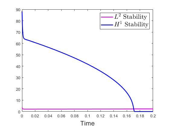
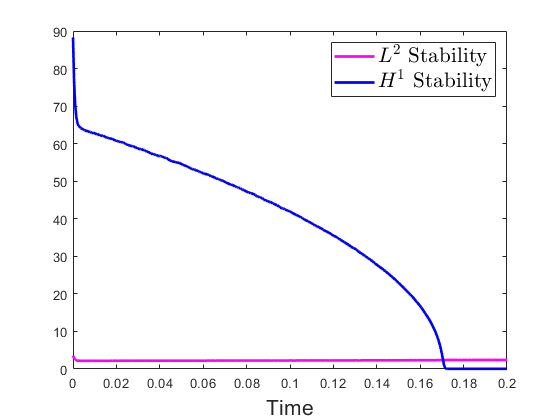
u_{0}(x,y)=\tanh(\frac{\sqrt{x^{2}+y^{2}}-0.6}{\sqrt{2}\epsilon}).

For this test, $F(u)=u-u^{3}$ is used as the nonlinear term, and $G(u)=\delta u$ is used as the diffusion term. In Figure 1, the zero-level sets of the evolution using two different levels of noise intensity are shown. One can observe that the average zero-level set is a shrinking circle for both levels of noise intensity. Figure 2 demonstrates the $\mathbb{E}L^{2}$ and $\mathbb{E}H^{1}$ stability for each time step. One can make the observation that they are both bounded. A one-sample $\mathbb{E}L^{2}$ and $\mathbb{E}H^{1}$ stability are provided in Figure 3. Those stability results are still bounded but they are not always decreasing over time.

Test 2. For this test, the initial condition is still in (5.1), and that $\epsilon=0.5$ . The drift term is changed to $F(u)=u-u^{11}$ , and the diffusion term is changed to $G(u)=\delta\sqrt{u^{2}+1}$ . In Figure 4, the $\mathbb{E}L^{2}$ and $\mathbb{E}H^{1}$ stability are given by the blue and pink solid lines, along with the maximum and minimum of those two stabilities given by upper and lower edges of the shaded red and blue regions. One can see that both the $\mathbb{E}L^{2}$ and $\mathbb{E}H^{1}$ stability are bounded.

Test 3. Consider the initial condition:

(5.2)

u_{0}(x,y)=\tanh(\frac{\sqrt{x^{2}+y^{2}}-0.8}{\sqrt{2}\epsilon}).

In this test, we use $\epsilon=0.3$ , $F(u)=u-u^{3}$ as the drift term, and $G(u)=\delta u$ as the diffusion term. The final time is $T=0.25$ . Table 1 demonstrates the error $\{\underset{0\leq n\leq N}{\sup}\mathbb{E}[||e^{n}||^{2}_{L^{2}(\mathcal{D})}]\}^{\frac{1}{2}}$ and the error $\{\mathbb{E}[\sum_{n=1}^{N}\tau||\nabla e^{n}||^{2}_{L^{2}(\mathcal{D})}]\}^{\frac{1}{2}}$ . The error $\{\underset{0\leq n\leq N}{\sup}\mathbb{E}[||e^{n}||^{2}_{L^{2}(\mathcal{D})}]\}^{\frac{1}{2}}$ is denoted by $L^{\infty}\mathbb{E}L^{2}$ , and the error $\{\mathbb{E}[\sum_{n=1}^{N}\tau||\nabla e^{n}||^{2}_{L^{2}(\mathcal{D})}]\}^{\frac{1}{2}}$ is denoted by $\mathbb{E}L^{2}H^{1}$ . By observingTable 1, one can see that the error orders for both $L^{\infty}\mathbb{E}L^{2}$ and $\mathbb{E}L^{2}H^{1}$ are 1.

	$L^{\infty}\mathbb{E}L^{2}$ error	order	$\mathbb{E}L^{2}H^{1}$ error	order
$\tau=0.025$	0.080163	-	0.054115	-
$\tau=0.0125$	0.038604	1.0542	0.027675	0.9675
$\tau=0.0625$	0.018036	1.0978	0.013978	0.9855
$\tau=0.03125$	0.008724	1.0479	0.007467	0.9045

Table 1: Test 3: Time step errors and rates of convergence of Test 3:

h=0.01,\epsilon=0.3,\delta=0.01,{T=0.25}

References

[1] P. L. Chow, Stochastic Partial Differential Equations, Chapman and Hall/CRC, 2007.
[2] R. Bank and H. Yserentant, On the $H^{1}$ -stability of the $L^{2}$ -projection onto finite element spaces, Numer. Math., 126 (2014), 361–381.
[3] S. Brenner and R. Scott, The Mathematical Theory of Finite Element Methods, Springer, 2008.
[4] C-E Bréhier and L. Goudenège, Analysis of some splitting schemes for the stochastic Allen-Cahn equation, Discrete Contin. Dyn. Syst. Ser. B, 24 (2019), 4169-4190.
[5] H. Brezis, Functional analysis, Sobolev spaces and partial differential equations, Springer, volume 2, 2011.
[6] Z. Brzeźniak, E. Carelli, and A. Prohl, Finite-element-based discretizations of the incompressible Navier–Stokes equations with multiplicative random forcing, IMA Journal of Numerical Analysis, 33.3 (2013): 771-824.
[7] P. Ciarlet, The finite element method for elliptic problems, Classics in Appl. Math., 40 (2002), 1–511.
[8] X. Feng, Y. Li and A. Prohl, Finite element approximations of the stochastic mean curvature flow of planar curves of graphs, Stoch. PDEs: Analysis and Computations, 2 (2014), 54–83.
[9] X. Feng, Y. Li and Y. Zhang, Finite element methods for the stochastic Allen-Cahn equation with gradient-type multiplicative noise, SIAM J. Numer. Anal., 55 (2017), 194–216.
[10] X. Feng, Y. Li and Y. Zhang. Strong convergence of a fully discrete finite element method for a class of semilinear stochastic partial differential equations with multiplicative noise, Journal of Computational Mathematics, 39(4):574-598, 2021.
[11] B. Gess. Strong solutions for stochastic partial differential equations of gradient type, Funct. Anal., 263, 2355–2383, 2012.
[12] I. Gyöngy and A. Millet, On discretization schemes for stochastic evolution equations, Potential analysis, 23 (2005), 99–134.
[13] I. Gyöngy, S. Sabanis and D. Šiška, Convergence of tamed Euler schemes for a class of stochastic evolution equations, Stochastics and Partial Differential Equations: Analysis and Computations, 4 (2016), 225–245.
[14] D. Higham, X. Mao and A. Stuart, Strong convergence of Euler-type methods for nonlinear stochastic differential equations, SIAM J. Numer. Anal., 40 (2002), 1041–1063.
[15] M. Hutzenthaler, A. Jentzen and P. Kloeden, Strong and weak divergence in finite time of Euler’s method for stochastic differential equations with non-globally Lipschitz continuous coefficients, Proceedings of the Royal Society A: Mathematical, Physical and Engineering Sciences, 467 (2010), 1563–1576.
[16] A. Jentzen and P. Pušnik, Strong convergence rates for an explicit numerical approximation method for stochastic evolution equations with non-globally Lipschitz continuous nonlinearities, IMA J. Numer. Anal., 40 (2020), 1–38.
[17] P. Kloeden and E. Platen, Numerical Methods for Stochastic Differential Equations, Springer, 1991.
[18] M. Kovács, S. Larsson and F. Lindgren, On the backward Euler approximation of the stochastic Allen-Cahn equation, J. Appl. Probab., 52 (2015), 323–338.
[19] M. Kovács, S. Larsson and F. Lindgren, On the discretisation in time of the stochastic Allen–Cahn equation, Mathematische Nachrichten, 291 (2018), 966–995.
[20] Z. Liu and Z. Qiao, Strong approximation of monotone stochastic partial differential equations driven by white noise, IMA J. Numer. Anal., 40 (2020), 1074–1093.
[21] A. Majee and A. Prohl, Strong rates of convergence for a space-time discretization of the stochastic Allen-Cahn equation with multiplicative noise, Comput. Methods Appl. Math., 18 (2018), 297–311.
[22] A. Majee and A. Prohl, Optimal Strong rates of convergence for a space-time discretization of the stochastic Allen-Cahn equation with multiplicative noise, Comput. Methods Appl. Math., 18 (2018), 297–311.
[23] X. Mao, Stochastic differential equations and applications, 2nd Edition, Elsevier, 2007.
[24] Mil’shtejn, Approximate integration of stochastic differential equations, Theory of Probability & Its Applications, 1975.
[25] D. Higham, X. Mao and A. Stuart. Strong convergence of Euler-type methods for nonlinear stochastic differential equations, SIAM J. Numer. Anal., 40 (2002), 1041–1063.
[26] G. J. Lord, C. E. Powel and T. Shardlow. An Introduction to Computational Stochastic PDEs, volume 50, Cambridge University Press, 2014.
[27] J. Printems, On the discretization in time of parabolic stochastic partial differential equations, M2AN Math. Model. Numer. Anal., 35 (2001), 1055–1078.
[28] L. Vo, Higher order time discretization method for the stochastic Stokes equations with multiplicative noise, arXiv 2211.02757, 2022.
[29] L. Vo, High moment and pathwise error estimates for fully discrete mixed finite element approximation of the stochastic Stokes equations with multiplicative noises, arXiv:2106.04534, 2021.
[30] J. Xu and L. Zikatanov, A monotone finite element scheme for convection-diffusion equations, Math. Comp., 68 (1999), 1429–1446.


(2.3a)	$\displaystyle\\|G({v})-G({w})\\|_{{\mathcal{K}}}$	$\displaystyle\leq C\\|{v}-{w}\\|_{{\mathcal{H}}}\,,$
(2.3b)	$\displaystyle\\|G({v})\\|_{{\mathcal{K}}}$	$\displaystyle\leq C\bigl{(}\\|{v}\\|_{{\mathcal{H}}}+1\bigr{)}\,.$

(2.11)		$\displaystyle\Bigl{\\|}DF(u(s))\Bigl{[}u(t)-u(s)-\int_{s}^{t}G(u(\xi))\,dW(\xi)\Bigr{]}\Bigr{\\|}^{2}_{L^{2}}$
	$\displaystyle=\int_{D}\Bigl{\|}(1-qu(s)^{q-1})\Bigl{[}u(t)-u(s)-\int_{s}^{t}G(u(\xi))\,dW(\xi)\Bigr{]}\Bigr{\|}^{2}\,dx$
	$\displaystyle\leq\int_{D}2(1+q^{2}\|u(s)\|^{2(q-1)})\Bigl{\|}\Bigl{[}u(t)-u(s)-\int_{s}^{t}G(u(\xi))\,dW(\xi)\Bigr{]}\Bigr{\|}^{2}\,dx$
	$\displaystyle\leq 2\Bigl{(}\int_{D}(1+q^{2}\|u(s)\|^{2(q-1)})^{2}\,dx\Bigr{)}^{\frac{1}{2}}\Bigl{\\|}u(t)-u(s)-\int_{s}^{t}G(u(\xi))\,dW(\xi)\Bigr{\\|}^{2}_{L^{4}}$
	$\displaystyle\leq 2\Bigl{(}\int_{D}2(1+q^{4}\|u(s)\|^{4(q-1)})\,dx\Bigr{)}^{\frac{1}{2}}\Bigl{\\|}u(t)-u(s)-\int_{s}^{t}G(u(\xi))\,dW(\xi)\Bigr{\\|}^{2}_{L^{4}}.$

(2.12)		$\displaystyle\mathbb{E}\Bigl{[}\Bigl{\\|}DF(u(s))\Bigl{[}u(t)-u(s)-\int_{s}^{t}G(u(\xi))\,dW(\xi)\Bigr{]}\Bigr{\\|}^{2}_{L^{2}}\Bigr{]}$
	$\displaystyle\leq\mathbb{E}\Bigl{[}2\Bigl{(}\int_{D}2(1+q^{4}\|u(s)\|^{4(q-1)})\,dx\Bigr{)}^{\frac{1}{2}}\Bigl{\\|}u(t)-u(s)-\int_{s}^{t}G(u(\xi))\,dW(\xi)\Bigr{\\|}^{2}_{L^{4}}\Bigr{]}$
	$\displaystyle\leq C_{q}\Bigl{(}\mathbb{E}\Bigl{[}\\|u(s)\\|^{4(q-1)}_{L^{4(q-1)}}\Bigr{]}\Bigr{)}^{\frac{1}{2}}\Bigl{(}\mathbb{E}\Bigl{[}\Bigl{\\|}u(t)-u(s)-\int_{s}^{t}G(u(\xi))\,dW(\xi)\Bigr{\\|}^{4}_{L^{4}}\Bigr{]}\Bigr{)}^{\frac{1}{2}}.$

(2.16)	$\displaystyle\mathbb{E}[\\|R_{2}\\|^{2}_{L^{2}}]$	$\displaystyle\leq C_{q}\mathbb{E}\bigl{[}\\|u(s)\\|^{2(q-2)}_{L^{4(q-2)}}\\|u(t)-u(s)\\|^{4}_{L^{8}}\bigr{]}+C_{q}\mathbb{E}\bigl{[}\\|u(t)-u(s)\\|^{2q}_{L^{2q}}\bigr{]}$
	$\displaystyle\leq C_{q}\Bigl{(}\mathbb{E}\bigl{[}\\|u(s)\\|^{4(q-2)}_{L^{4(q-2)}}\bigr{]}\Bigr{)}^{\frac{1}{2}}\Bigl{(}\mathbb{E}\bigl{[}\\|u(t)-u(s)\\|^{8}_{L^{8}}\bigr{]}\Bigr{)}^{\frac{1}{2}}$
	$\displaystyle\qquad\qquad+\mathbb{E}\bigl{[}\\|u(t)-u(s)\\|^{2q}_{L^{2q}}\bigr{]}$
	$\displaystyle\leq C(\|t-s\|^{4\theta_{1}}+\|t-s\|^{2q\theta_{1}})\leq C\|t-s\|^{4\theta_{1}},$

(3.8)	$\displaystyle\mathbb{E}[{\tt III}]$	$\displaystyle\leq\frac{C}{\tau}\mathbb{E}\bigl{[}\\|DG(u^{n})G(u^{n})\\|^{2}_{L^{2}}\|(\Delta W_{n})^{2}-\tau\|^{2}\bigr{]}+\frac{\tau}{4}\mathbb{E}\bigl{[}\\|\Delta u^{n+1}\\|^{2}_{L^{2}}\bigr{]}$
	$\displaystyle\leq\frac{C}{\tau}\mathbb{E}\bigl{[}\\|G(u^{n})\\|^{2}_{L^{2}}\|(\Delta W_{n})^{2}-\tau\|^{2}\bigr{]}+\frac{\tau}{4}\mathbb{E}\bigl{[}\\|\Delta u^{n+1}\\|^{2}_{L^{2}}\bigr{]}$
	$\displaystyle\leq C\tau\mathbb{E}\bigl{[}\\|\nabla u^{n}\\|^{2}_{L^{2}}\bigr{]}+\frac{\tau}{4}\mathbb{E}\bigl{[}\\|\Delta u^{n+1}\\|^{2}_{L^{2}}\bigr{]},$

Higher order time discretization method for a class of semilinear stochastic partial differential equations with multiplicative noise

Abstract

keywords:

AMS:

1 Introduction

2 Preliminaries

Lemma 1.

Proof.

3 Semi-discretization in time

3.1 Formulation of the proposed method

Remark 3.1.

Lemma 2.

Proof.

Lemma 3.

Proof.

3.2 Error estimates for Algorithm 1

Theorem 4.

Proof.

4 Fully discrete finite element discretization

4.1 Stability estimates for the pp-th moment of the H1H^{1}-seminorm of uhnu_{h}^{n}

Theorem 5.

Proof.

Theorem 6.

Proof.

4.2 Stability estimates for the pp-th moment of the L2L^{2}-norm of uhnu_{h}^{n}

Theorem 7.

Proof.

Theorem 8.

Proof.

4.3 Error estimates of the finite element approximation

Theorem 9.

Proof.

4.4 Global error estimates

Theorem 10.

5 Numerical Experiments

References

4.1 Stability estimates for the $p$ -th moment of the $H^{1}$ -seminorm of $u_{h}^{n}$

4.2 Stability estimates for the $p$ -th moment of the $L^{2}$ -norm of $u_{h}^{n}$