Higher-order exceptional point in a blue-detuned non-Hermitian cavity optomechanical system
Abstract
Higher-order exceptional points (EPs) in non-Hermitian systems have attracted great interest due to their advantages in sensitive enhancement and distinct topological features. However, realization of such EPs is still challenged because more fine-tuning parameters is generically required in quantum systems, compared to the second-order EP (EP2). Here, we propose a non-Hermitian three-mode optomechanical system in the blue-sideband regime for predicting the third-order EP (EP3). By deriving the pseudo-Hermitian condition for the proposed system, one cavity with loss and the other one with gain must be required. Then we show EP3 or EP2 can be observed when the mechanical resonator (MR) is neutral, loss or gain. For the neutral MR, we find both two degenerate or two non-degenerate EP3s can be predicted by tuning system parameters in the parameter space, while four non-degenerate EP2s can be observed when the system parameters deviate from EP3s, which is distinguished from the previous study in the red-detuned optomechanical system. For the gain (loss) MR, we find only two degenerate EP3s or EP2s can be predicted by tuning enhanced coupling strength. Our proposal provides a potential way to predict higher-order EPs or multiple EP2s and study multimode quantum squeezing around EPs using the blue-detuned non-Hermitian optomechanical systems.
I introduction
Cavity optomechanical (COM) systems, emerged as a promising platform in quantum information science, have been paid considerable attention both theoretically and experimentally Aspelmeyer . The simplest COM system is made up of a mechanical resonator (MR) nonlinearly coupled to a cavity via radiation pressure, which can be well controlled by strong driving fields. In such mystical systems, abundant effects including sensing Schreppler-2014 ; Wu-2017 ; Gil-Santos-2020 ; Fischer-2019 , ground-state cooling Chan-2011 ; Teufel-2011 , squeezed light generation Purdy-2014 ; Safavi-Naeini-2013 ; Aggarwal-2020 , nonreciprocal transport Xu-2019 ; Shen-2016 , optomechanically induced transparency Kronwald-2013 ; Weis-2010 ; Liuy-2013 , coupling enhancement Xiong-2021 ; Lu-2013 ; Xiong2-2021 , and nonlinear behaviors (e.g., bi- and tristability and chaos ) Lu-2015 ; Xiong3-2016 have been investigated.
In addition, COM systems have shown huge potential in studying exceptional points (EPs) of non-Hermitian systems Xiongwei-2021 ; Jing-2014 ; Xu-2016 ; LYL-2017 ; ZhangJQ-2021 ; XuH-2021 ; Xuxw-2015 , at which both eigenvalues and eigenvectors coalesce. This is due to the fact that practical COM systems can be characterized by effective non-Hermitian Hamiltonians when decoherence arising from surrounding environment is considered. Moreover, the driven COM systems can provide fine-tuning parameters for requirement of realizing EPs, assisted by strong driving fields. Owing to these, EPs have been intensively studied in COM systems, especially for the second-order EPs (EP2s) Jing-2014 ; Xu-2016 ; LYL-2017 ; ZhangJQ-2021 ; XuH-2021 ; Xuxw-2015 where two eigenvalues and the corresponding eigenvectors coalesce Minganti-2019 ; Zhang-2021 ; Ozdemir-2019 ; Mostafazadeh1-2002 ; Mostafazadeh2-2002 ; Konotop-2016 ; Bender-2013 ; Parto-2021 ; Bergholtz-2021 ; Wiersig-2020 ; Feng-2017 ; El-Ganainy-2018 . Besides, EP2s are also studied in other systems Doppler-2016 ; Zhang-2017 ; Harder-2017 ; Quijandria-2018 ; Zhang-2019-2 ; Naghiloo-2019 ; ZhangGQ . Around EP2s, lots of fascinating phenomena like unidirectional invisibility Peng-2014 ; Lin-2011 ; Chang-2014 , single-mode lasing Feng-2014 ; Hodaei-2014 , sensitivity enhancement Chen-2017 ; Hokmabadi-2019 , energy harvesting Fern-2021 , protecting the classification of exceptional nodal topologies Marcus-2021 , electromagnetically induced transparency Guo-2009 ; Wang-2019 ; Wang1-2020 ; Lu-2021 , and quantum squeezing Miranowicz-2019 ; Mukherjee-2019 ; Luo-2022 can be studied.
Instead of EP2s, non-Hermitian systems can also host higher-order EPs, where more than two eigenmodes coalesce into one Graefe-2008 ; Heiss-2008 ; Demange-2012 ; Heiss-2016 ; Jing-2017 ; Ge-2015 ; Lin-2016 ; Quiroz-2019 ; Bian-2020 . It has been shown that higher-order EPs can exhibit greater advantages than EP2s in spontaneous emission enhancement Lin-2016 , sensitive detection Hodaei-2017 ; Zeng-2021 ; Wang-2021 ; Zeng-2019 , topological characteristics Ding-2016 ; Delplace-2021 ; Mandal-2021 . With these superiorities, higher-order EPs are being intensively studied in various systems Roy-2021 ; Zhong-2020 ; Zhang-2020 ; Pan-2019 ; Zhang-2019 ; Kullig-2019 ; Kullig-2018 ; Schnabel-2017 ; Nada-2017 ; Wang-2020 but attract less attention in non-Hermitian COM systems. For this, how to construct higher-order EPs in non-Hermitian COM systems is strongly demanded.
We also note that EPs in non-Hermitian COM systems, including EP2s and EP3s, are mainly focused in the red-sideband regime Xiongwei-2021 ; Jing-2014 . In this regime, fast oscillating terms related to mode squeezing are neglected. This limits nonclassical quantum effects such as quantum squeezing investigation around EPs. For this, we here theoretically propose a paradigmatic COM system consisting of a MR coupled to two cavities via radiation pressure for predicting EP3s, where two cavities are respectively passive (loss) and active (gain), and driven by two blue-detuned classical fields. First, we derive an effective non-Hermitian Hamiltonian for the proposed COM system and analytically give the pseudo-Hermitian condition of the proposed COM system in the general case. Then, three scenarios are specifically considered in the pseudo-Hermitian condition: (i) the neutral MR; (ii) the passive MR; (iii) the active MR. In case (i), the proposed non-Hermitian COM system with symmetric coupling strength can host both two degenerate EP3s and two non-degenerate EP3s in the parameter space. When we tune the system parameters deviation from the critical paraters at EP3s, four non-degenerate EP2s can be predicted, which is different from the situation in the red-sideband non-Hermitian COM system. For the cases (ii) and (iii), the proposed non-Hermitian COM system is required to have asymmetric coupling strength for satisfying pseudo-Hermitian condition. We find only two degenerate EP3s or two degenerate EP2s can be predicted. By investigating the effects of system paramters on EP3s or EP2s, we find large coupling strength or large frequency detuning is benefit to observe EPs more clearly. Our proposal provides a promising path to study nonclassical quantum effects around EP2s and EP3s in non-Hermitian COM systems, and it is the first scheme to study higher-order EPs in the blue-detuned COM system, although two-mode quantum squeezing has been investigated in a system with pseudo-anti-parity-time symmetry Luo-2022 .
This paper is organized as follows. In Sec. II, the model is described and the system effective Hamiltonian is given. Then we derive the pesudo-Hermitian condition for the considered non-Hermitian COM system in Sec. III. In Sec. IV, critical parameters of the proposed COM system at EP3 are anatically derived. In Sec. V, phase diagram of the descriminant for the characteristic equation is studied to predict EP3 and EP2. In Sec. VI, EP3 and EP2 in three cases are specifically studied. Finally, a conclusion is given in Sec. VII.
II Model and Hamiltonian
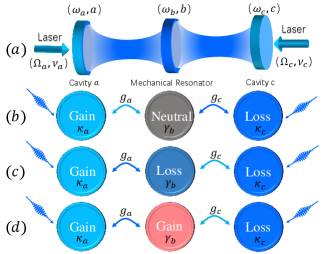
We consider an experimental three-mode optomechanical system Dong-2012 ; Hill-2012 ; Andrews-2014 consisting of two driven cavities (labeled as cavity and cavity ) coupled to a MR with frequency via radiation pressure (see Fig. 1). At the rotating frame respect to two laser fields, the Hamiltonian of the total system can be written as (setting ) Zhangk-2015
| (1) |
where , with being the frequency of the cavity and the frequency of the laser field acting on the cavity , is the frequency detuning of the cavity from the laser field acting on the cavity . and are the single-photon optomechanical coupling strengths of the MR coupled to the cavity and cavity , respectively. The operators and are the annihilation and creation operators of the cavity . The last term in Eq. (1) represents the coupling between two cavities and two laser fields with Rabi frequencies and . As we are interested in the blue-sideband regime of the proposed COM system, thus is assumed below.
In the strong-field limit, the nonlinear COM system can be linearized by writing each operator as the expectation value () plus the corresponding fluctuation (). Neglecting the higher-order fluctuations, the linearized Hamiltonian including dissipations can be given by (see details in the Appendix)
| (2) |
Here, fast oscillating terms have been discarded with the condition and , where is the effective frequency detuning of the cavity shifted by the displacement of the mechanical resonator, and is the effective optomechanical coupling strength enhanced by the photon number in the cavity . This effective Hamiltonian is the typical three-mode squeezing Hamiltonian without dissipations. For convenience, we assume and to be real, which can be realized by tuning the phase of two laser fields.
III Pseudo-Hermitian condition
The effective Hamiltonian in Eq. (2) can also be equivalently expressed as
| (3) |
is just the matrix form of . For the non-Hermitian Hamiltonian in Eq. (3), three eigenvalues can be predicted. When these three eigenvalues are all real, or one is real and the other two are a complex-conjugate pair, the considered three-mode optomechanical system characterized by the Hamiltonian in Eq. (2) or Eq. (3) is pseudo-Hermitian Mostafazadeh1-2002 ; Mostafazadeh2-2002 . For the pseudo-Hermitian systems, the characteristic polynomial equation
| (4) |
is the same as
| (5) |
where is the complex conjugate transpose of , is a identity matrix, and denotes the eigenvalue of the effective Hamiltonian . By expanding Eqs. (4) and (5), and comparing the corresponding coefficients, we can obtain
| (6) | ||||
By setting
| (7) |
Eq. (III) can be further simplified as
| (8) | |||
Obviously, only when the conditions in Eq. (III) are simutaneously satisfied, the considered three-mode optomechanical system is pseudo-Hermitian. From the first condition in Eq. (III), we can see that the decay rates from the cavity , the mecahanical resonator and the cavity are required to be balanced. This means gain effect must be introduced to the considered system. From the third condition, is obtained, which shows one loss cavity and the other gain cavity are always needed to satisfy the pseudo-Hermitian condition for the proposed COM system in the blue-sideband regime. This situation is completely different from the previous study of EPs using a COM system in the red-sideband regime. Without loss of generality, the cavity with gain, and the cavity with loss are taken, i.e., and . From the third equation in Eq. (III), it is not difficult to find the fact that when , which indicates that the coupling strengths between the MR and two cavities must be uniform, i.e., . When ,
| (9) |
is directly given by the third equality in Eq. (III), which in turn gives rise to a boundary for the parameter or equivalently and . Such the boundary can be achieved here owing to the tunable parameters and .
IV critical parameters at EP3
When the pseudo-Hermitian conditions in Eq. (III) are satisfied and is defined, the characteristic equation in Eq. (4) reduces to
| (10) |
where
| (11) | ||||
According to Cardano’s formula kORN-1968 , the solutions of this characteristic equation is determined by the discriminant
| (12) |
where
| (13) |
For , Eq. (10) has three real roots. But for , Eq. (10) only has one real root and the other two are complex roots. Interestingly, three roots coalesce to the same value at with , which is so-called EP3. For the case of but and , only two roots coalesce to the value , corresponding to EP2.
Below we analytically derive the critical parameters at EP3. When EP3 appears at , we have
| (14) |
Comparing coefficients of this equation with Eq. (10),
| (15) |
are obtained. The first equation directly leads to
| (16) |
Substituting this solution back into the second equation in Eq. (15), the critical coupling strength at EP3 is given by
| (17) |
where
| (18) |
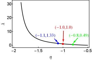
is derived from the third equation in Eq. (III). As , so the minimal value of for predicting EP3 is
| (19) |
At EP3, the parameter is required to meet
| (20) |
which is obtained by substituting the solution in Eq. (16) back into the third equality in Eq. (15). To see the dependent relationship between and at EP3 more clearly, we plot as a function of in Fig. 2. Obviously, monotonously decreases with the absolute value of . Eq. (20) also requires to satisfy
| (21) |
Combine Eqs. (9) and (21) together, the parameter for predicting EP3 can take
| (22) |
leading to
| (23) |
The corresponding value of is given by Eq. (20).
V Phase diagram for prediction of EP3 and EP2
Next, we numerically predict EP3 and EP2 via phase diagram of the discriminant [see Eq. (12)] with in the three cases given by Eq. (22).
V.1
When , i.e., , two optomechanical cavities are gain-loss balanced, Eq. (III) reduces to
| (24) |
For the condition , it is difficult to be perfectly satisfied. But for COM systems, the decay rate of the MR is in general much smaller than the decay rate of the optomechanical cavity, i.e., . Therefore, we can safely ignore the effect of the decay rate of the MR on EP3, and thus we assume . In addition, the coefficients in Eq. (IV) are simplified as
| (25) |
Correspondingly, the discriminant in Eq. (12) becomes
| (26) |
and in Eq. (13) are
| (27) | ||||
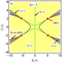
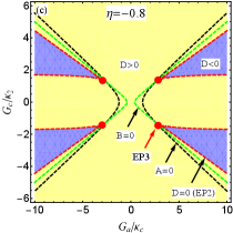
In Fig. 3(a), we plot the phase diagram determined by the sign of the discriminant [see Eq. (26)] vs the normalized parameters and , where the purple (yellow) region indicates . The boundary curve in red means . The curves in black and green respectively denote and . Obviously, three curves have four cross points, that is, four EP3s in the parameter space can be found according to the Cardano’s formula kORN-1968 . Also, EP2 can be predicted by the red curve only (i.e., , but and ).
V.2
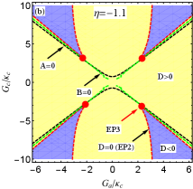
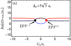
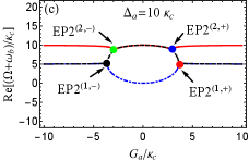
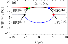
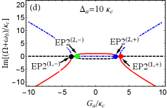
For the more realistic case, is further considered. This indicates that two optomechanical cavities are gain-loss unbalanced. According to Eq. (22), we can discuss the case of in two scenarios, i.e., (i) (or ); (ii) (or ). The first scenario indicates that the loss MR and (i.e., ) are needed to predict EP3 in our proposed COM system. On the contrary, the gain MR and (i.e., ) is required in the second scenario. As examples, we take and [see the blue and green dots in Fig. 2]. Then we plot the phase diagram of the discriminant with [see Fig. 3(b)] and [see Fig. 3(c)] vs the normalized parameters and , where , , and are shown by the red, black and green curves, respectively. The purple (yellow) region means . Obviously, four EP3s [see the red dots] produced by three curves, at which , can be predicted in both Figs. 3(b) and 3(c) by tuning and . This can be realized because both and are tunable coupling strengths via tuning the Rabi frequencies of the two laser fields. When we deviate () from () at EP3, EP2 emerges [see the red curve only in Figs. 3(b) and 3(c)]. When one parameter is fixed in Figs. 3(a-c), we can easily find that only two EP3s or four EP2s can be observed by varying the other parameter, which is different from the case considered in the red-detuned COM system.
VI EP3 and EP2 in the blue-sideband three-mode optomechanical system
VI.1
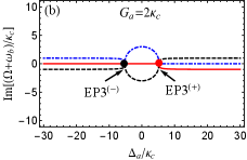
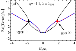
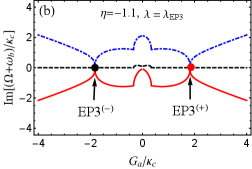
In Fig. 3(a), we have predicted that EP3 and EP2 can be observed in our considered system for the case of . For clarity, we below study the behavior of three eigenvalues of the Hamiltonian given by Eq. (2) with different frequency detunings and coupling strengths .
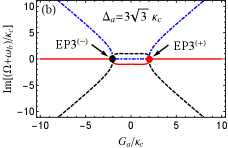
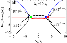
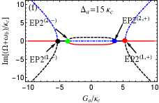
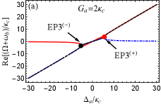
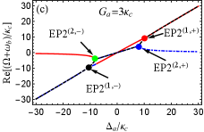
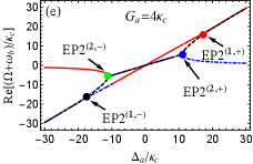
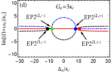
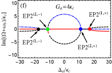
In Fig. 4, we plot the real and imaginary parts of the eigenvalue () as a function of the normalized parameter with . For simplicity, we assume that the red, blue and black curves respectively denote three eigenvalues and for the Hamiltonian hereafter. For [see Figs. 4(a) and 4(b)], is real and the other two eigenvalues ( and ) are a complex-conjugate pair in the region of or . But when , becomes real, and , become a complex-conjugate pair. At the points [see the red and black dots in Figs. 4(a) and 4(b)], three eigenvalues coalesce to one value, i.e., , corresponding to two degenerate EP3s. It is not difficult to verify that and at two EP3s. Then we increase to [see Figs. 4(c) and 4(d)] for deviation from EP3s, that is, but and . For or , is real, and are a complex-conjugate pair, At [see the red and black dots in Figs. 4(c) and 4(d)], and coalesce to , corresponding to two degenerate EP2s. By increasing to or , the real parts of and bifurcate into two values. At [see the blue and green dots in Figs. 4(c) and 4(d)], and coalesce to the value , corresponding another two degenerate EP2s. When , is real and the other two eigenvalues and are complex conjugates. We also find the separation between arbitrary two EP2s can be increased using larger such as [see Figs. 4(c-f)], which indicates that larger is benifit to distinguishably observe multiple EP2s.
In Fig. 5, we also plot the real and imaginary parts of the eigenvalue () vs the normalized parameter with different . For [see Figs. 5(a) and 5(b)], is real, and , are a complex-conjugate pair when . At [see the black dot in Figs. 5(a) and 5(b)], three eigenvalues coalesce to , corresponding to EP3. When , and become a complex-conjugate pair again, and is real. But when , becomes real, and are a complex-conjugate pair. At , three eigenvalues remerge into the same value . By increasing to [see the red dot in Figs. 5(c) and 5(d)], two EP3s in Figs. 5(a) and 5(b) split into four EP2s. Specifically, is real, and are a complex-conjugate pair when . At [see the black dot in Figs. 5(c) and 5(d)], and coalesce to , corresponding to the first EP2. When , three eigenvalues are all real but have different values. At [see the green dot in Figs. 5(c) and 5(d)], and coalesce to , corresponding to the second EP2. For , is real, and are a complex-conjugate pair. At [see the blue dot in Figs. 5(c) and 5(d)], and remerge into one value , corresponding to the third EP2. By tuning to [see the red dot in Figs. 5(c) and 5(d)], two different real eigenvalues (i.e., and ) in degenerate as , corresping to the fourth EP2. When exceeds , becomes real, and are a complex conjugates. By considering a larger such as [see Figs. 5(e) and 5(f)], we find EP2s can be distinguished more easily. This indicates that larger coupling strength can also be used to observe EP2s clearly, similar to the role of the above discussed frequency detuning .
VI.2
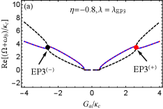
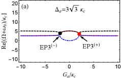
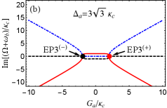
For the case of , we also have numerically proved that EP3 and EP2 can be predicted in our proposed blue-sideband optomechanical system by respectively taking and as examples in Figs. 3(b) and 3(c). Here we further specifically study EP3 and EP2 by investigating the eigenvalues of with and .
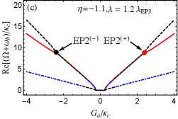
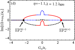
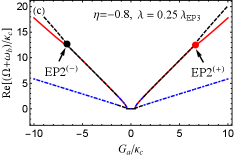
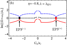
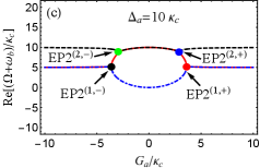
For (or equivalently ), which leads to and . we plot the real and imaginary parts of the eigenvalue () vs the normalized parameter with different in Fig. 6. From Figs. 6(a) and 6(b) in which , we can see that the eigenvalue denoted by the black curve is always real for arbitrary , and the other two eigenvalues ( and ) are a complex-conjugate pair except for at points . At these two points, three eigenvalues coalesce into one value , corresponding to two EP3s. When we take , slightly derivating from at EP3s, the condition for predicting EP3s is broken, thus EP3 disappears. According to Fig. 3(b), EP2 can be observed. In Figs. 6(c) and 6(d), we plot the real and imaginary parts of the eigenvalue () vs the normalized parameter with . It is not difficult to find that three eigenvalues are all real when or . At , and coalesce to , corresponding to two EP2s. When , the real parts of and are still degenerate, but their imaginary parts bifurcate into two values.
VII Discussion and Conclusion
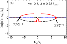
Note that our studies are constrainted in the pseudo-Hermitian condition, which can ensure the emergence of EPs in our proposed non-Hermitian COM system. But actually, the strict pseudo-Hermitian condition in general can not be fully satisfied, which means that the pseudo-Hermitian condition is broken [see Eq. (III) or Eq. (III)]. For example, the gain and loss in Eq. (III) are not balanced, i.e., . In this situation, we find that both EP3 and EP2 can also be predicted in our setup, as shown in Fig. 8 where and is taken. This shows that EPs in our proposal are robust against the slightly unbalanced gain and loss, which also reveals that the pseudo-Hermitian condition is neither sufficient nor necessary condition for predicting EPs. For the case of , we also numerically check it, and the same result is obtained.
In summary, we have proposed a blue-detuned non-Hermitian cavity optomechanical system consisting of a MR coupled to both a passive (loss) and an active (gain) cavities via radiation pressure for predicting EP3s. Under the pseudo-Hermitian condition, the cases of the neural, loss and gain MRs are considered. By investigating the phase diagram of the discriminant, we find that both two degenerate or two non-degenerate EP3s can be predicted by tuning system parameters in the parameter space for the neutral MR. Also, four non-degenerate EP2s can be observed when system parameters deviate from EP3s, which is distinguished from the previous study in the red-detuned optomechanical system. For the gain (loss) MR, we find only two degenerate EP3s or EP2s can be predicted by tuning enhanced coupling strength. By studying the effect of parameters on EP3s or EP2s, we show that large parameters, such as frequency detuning and enhanced optomechanical coupling strength, can be employed to observe EPs more clearly. Our proposal is the first scheme to study higher-order EPs in the blue-detuned COM system, and it provides a potential way to investigate multimode quantum squeezing effects around higher-order EPs
ACKNOWLEDGMENTS
This paper is supported by the key program of the Natural Science Foundation of Anhui (Grant No. KJ2021A1301), the National Natural Science Foundation of China (Grants No. 12205069, No. 11904201 and No. 12104214), and the Natural Science Foundation of Hunan Province of China (Grant No. 2020JJ5466).
Appendix A The derivation of the effective Hamiltonian
In this Appendix, we derive the effective Hamiltonian given by Eq. (2) in the main text. Following the quantum Langevin equation method Benguria-1981 , the dynamics of the proposed system including dissipations can be given by
| (A1) | ||||
where is the decay rate of the cavity , and is the decay rate of the MR. Note that when one of the cavities such as the cavity is subject to the dissipative gain, its corresponding dynamics in Eq. (A) should be corrected as Gardiner-2000 , which is different from the first equation in Eq. (A). , and are vacuum input noises with zero expectation value, i.e., . To linearize the nonlinear equations in Eq. (A), we write the operators , , and as , where , , are steady-state values, and , , are fluctuation operators. Then we substitute these transformations into Eq. (A). In the strong-field limit, i.e., , higher-order fluctuation terms can be safely neglected. Thus, the dynamics of the fluctuation operators in Eq. (A) can be linearized as
| (A2) | ||||
where and are the effective frequency detunings of the cavity and the cavity , respectively, shifted by the displacement of the MR. In general, such frequency shifts are tiny due to weak single-photon optomechanical coupling strengths. Experimentally, are used. and are the effective enhanced optomechanical coupling strengths, which can be tuned by the amplitudes of the two laser fields. Under the condition and , the fast oscillating terms in Eq. (A) can be neglected, then Eq. (A) reduces to
| (A3) |
By rewriting the equations of motion in Eq. (A) as , , and , the effective non-Hermitian Hamiltonian in the blue-sideband regime can be obtained,
| (A4) |
which is just the effective Hamitonian in Eq. (2).
Appendix B Stability
From Eq. (A), we can obtain the following equations,
| (B5) | ||||
By setting
| (B6) |
Eq. (B) can be rewritten as
| (B7) |
where , , and is given by
| (B8) |
The considered COM system is stable only when the real parts of the eigenvalues of the matrix are all negative, which can be judged by the Routh-Hurwitz criterion Gradshteyn . To using this criterion, we expand the characteristic equation as , where the coefficients with can be derived using straightforward but tedious algebra. Interestingly, we find when , which breaks the Routh-Hurwitz criterion for prediction of the stability. This indicates that when the pseudo-Hermitian condition is strictly satisfied, the considered system is possibly unstable. To ensure the system stable, is required in experiment. This requirement can be achieved when two cavities are gain-loss balanced and the loss mechanical resonatr is employed. Although the pseudo-Hermitian condition is broken, EP3s or EP2s can also be predicted (see Fig. 8). Other stable conditions obtained from the Routh-Hurwitz criterion can be well satisfied. This is due to the tunable frequency detunings and linearized optomechanical coupling strengths via tuning driving fields.
References
- (1) M. Aspelmeyer, T. J. Kippenberg, and F. Marquardt, Cavity optomechanics, Rev. Mod. Phys. 86, 1391 (2014).
- (2) S. Schreppler, N. Spethmann, N. Brahms, T. Botter, M. Barrios, and D. M. Stamper-Kurn, Optically measuring force near the standard quantum limit. Science 344, 1486 (2014).
- (3) M. Wu, N. L.Y. Wu, T. Firdous, F. F. Sani, J. E. Losby, M. R. Freeman, and P. E. Barclay, Nanocavity optomechanical torque magnetometry and radiofrequency susceptometry, Nat. Nanotechnol. 12, 127 (2017).
- (4) E. Gil-Santos, J. J. Ruz, O. Malvar, I. Favero, A. Lemaître, P. M. Kosaka, S. García-López, M. Calleja, and J. Tamayo, Optomechanical detection of vibration modes of a single bacterium, Nat. Nanotechnol. 15, 469 (2020).
- (5) R. Fischer, D. P. McNally, C. Reetz, G. G.T. Assumpção, T. Knief, Y. Lin, and C. A. Regal, Spin detection with a micromechanical trampoline: Towards magnetic resonance microscopy harnessing cavity optomechanics, New J. Phys. 21, 43049 (2019).
- (6) J. Chan, T. P. M. Alegre, A. H. Safavi-Naeini, J. T. Hill, A. Krause, S. Gröblacher, M. Aspelmeyer, and O. Painter, Laser cooling of a nanomechanical oscillator into its quantum ground state, Nature (London) 478, 89 (2011).
- (7) J. D. Teufel, T. Donner, D. Li, J. W. Harlow, M. S. Allman, K. Cicak, A. J. Sirois, J. D. Whittaker, K. W. Lehnert, and R. W. Simmonds, Sideband cooling of micromechanical motion to the quantum ground state, Nature (London) 475, 359 (2011).
- (8) T. P. Purdy, P. L. Yu, R. W. Peterson, N. S. Kampel, and C. A. Regal, Strong optomechanical squeezing of light, Phys. Rev. X 3, 031012 (2013).
- (9) A. H. Safavi-Naeini, S. Gröblacher, J. T. Hill, J. Chan, M. Aspelmeyer, and O. Painter, Squeezed light from a silicon micromechanical resonator, Nature (London) 500, 1852013).
- (10) N. Aggarwal, T. J. Cullen, J. Cripe, G. D. Cole, R. Lanza, A. Libson, D. Follman, P. Heu, T. Corbitt, and N. Mavalvala, Room-temperature optomechanical squeezing, Nat. Phys. 16, 784 (2020).
- (11) H. Xu, L. Jiang, A. A. Clerk, and J. G. E. Harris, Nonreciprocal control and cooling of phonon modes in an optomechanical system, Nature (London) 568, 65 (2019).
- (12) Z. Shen, Y. L. Zhang, Y. Chen, C. L. Zou, Y. F. Xiao, X. B. Zou, F. W. Sun, G. C. Guo, and C. H. Dong, Experimental realization of optomechanically induced non-reciprocity, Nat. Photonics 10, 657 (2016).
- (13) A. Kronwald and F. Marquardt, Optomechanically Induced Transparency in the Nonlinear Quantum Regime, Phys. Rev. Lett. 111, 133601 (2013).
- (14) S. Weis, R. Riviere, S. Deleglise, E. Gavartin, O. Arcizet, A. Schliesser, and T. J. Kippenberg, Optomechanically Induced Transparency, Science 330, 1520 (2010).
- (15) Y. Liu, M. Davanço, V. Aksyuk, and K. Srinivasan, Electromagnetically Induced Transparency and Wideband Wavelength Conversion in Silicon Nitride Microdisk Optomechanical Resonators, Phys. Rev. Lett. 110, 223603 (2013).
- (16) W. Xiong, J. Chen, B. Fang, M. Wang, L. Ye, and J. Q. You, Strong tunable spin-spin interaction in a weakly coupled nitrogen vacancy spin-cavity electromechanical system, Phys. Rev. B 103, 174106 (2021).
- (17) X. Y. L, W. M. Zhang, S. Ashhab, Y. Wu, and F. Nori, Quantum-criticality-induced strong Kerr nonlinearities in optomechanical systems, Sci. Rep. 3, 2943 (2013).
- (18) J. Chen, Z. Li, X. Q. Luo, W. Xiong, M. Wang, and H. C. Li, Strong single-photon optomechanical coupling in a hybrid quantum system, Opt. Express 29, 32639 (2021).
- (19) W. Xiong, D. Y. Jin, Y. Qiu, C. H. Lam, and J. Q. You, Cross-Kerr effect on an optomechanical system, Phys. Rev. A 93, 023844 (2016).
- (20) X. Y. Lü, H. Jing, J. Y. Ma, and Y. Wu, -Symmetry Breaking Chaos in Optomechanics, Phys. Rev. Lett. 114, 253601 (2015).
- (21) W. Xiong, Z. Li, Y. Song, J. Chen, G. Q. Zhang, M. Wang, Higher-order exceptional point in a pseudo-Hermitian cavity optomechanical system, Phys. Rev. A 104, 063508 (2021).
- (22) H. Jing, ¸S. K. Özdemir, X.-Y. Lü, J. Zhang, L. Yang, and F. Nori, -Symmetric Phonon Laser, Phys. Rev. Lett. 113, 053604 (2014).
- (23) Y. L. Liu, R. Wu, J. Zhang, S. K. Özdemir, L. Yang, F. Nori, and Y. X. Liu, Controllable optical response by modifying the gain and loss of a mechanical resonator and cavity mode in an optomechanical system, Phys. Rev. A 95, 013843 (2017).
- (24) H. Xu, D. Mason, L. Jiang, and J. G. E. Harris, Topological energy transfer in an optomechanical system with exceptional points, Nature (London) 537, 80 (2016).
- (25) J. Q. Zhang, J. X. Liu, H. L. Zhang, Z. R. Gong, S. Zhang, L. L. Yan, S. L. Su, H. Jing, and M. Feng, Synthetic -Symmetry and Nonreciprocal Amplification in Optomechanics, arXiv:2107.10421.
- (26) H. Xu, D.-G. Lai, Y.-B. Qian, B.-P. Hou, A. Miranowicz, and F. Nori, Optomechanical dynamics in the -and broken--symmetric regimes, Phys. Rev. A 104, 053518 (2021).
- (27) X. W. Xu, Y. X. Liu, C. P. Sun, and Y. Li, Mechanical -symmetry in coupled optomechanical systems, Phys. Rev. A 92, 013852 (2015).
- (28) F. Minganti, A. Miranowicz, R. W. Chhajlany, and F. Nori, Quantum exceptional points of non-Hermitian Hamiltonians and Liouvillians: The effects of quantum jumps, Phys. Rev. A 100, 062131 (2019).
- (29) G. Q. Zhang, Z. Chen, D. Xu, N. Shammah, M. Liao, T. F. Li, L. Tong, S. Y. Zhu, F. Nori, and J. Q. You, Exceptional Point and Cross-Relaxation Effect in a Hybrid Quantum System, PRX Quantum 2, 020307 (2021).
- (30) S. K. Özdemir, S. Rotter, F. Nori, and L. Yang, Parity-time symmetry and exceptional points in photonics, Nat. Mater. 18, 783 (2019).
- (31) A. Mostafazadeh, Pseudo-Hermiticity versus -symmetry: The necessary condition for the reality of the spectrum of a non-Hermitian Hamiltonian, J. Math. Phys. 43, 205 (2002).
- (32) A. Mostafazadeh, Pseudo-Hermiticity versus -symmetry II: A complete characterization of non-Hermitian Hamiltonians with a real spectrum, J. Math. Phys. 43, 2814 (2002).
- (33) V. V. Konotop, J. Yang, and D. A. Zezyulin, Nonlinear waves in -symmetric systems, Rev. Mod. Phys. 88, 035002 (2016).
- (34) C. M. Bender, B. K. Berntson, D. Parker, and E. Samuel, Observation of phase transition in a simple mechanicalsystem, Am. J. Phys. 81, 173 (2013).
- (35) M. Parto, Y. G. N. Liu, B. Bahari, M. Khajavikhan, and D. N. Christodoulides, Non-Hermitian and topological photonics: Optics at an exceptional point, Nanophotonics 10, 403 (2021).
- (36) E. J. Bergholtz, J. C. Budich, and F. K. Kunst, Exceptional topology of non-Hermitian systems, Rev. Mod. Phys. 93, 015005 (2021).
- (37) J. Wiersig, Review of exceptional point-based sensors, Photonics Res. 8, 1457 (2020).
- (38) L. Feng, R. El-Ganainy, and L. Ge, Non-Hermitian photonics based on parity-time symmetry, Nat. Photonics 11, 752 (2017).
- (39) R. El-Ganainy, K. G. Makris, M. Khajavikhan, Z. H. Musslimani, and D. N. Christodoulides, Non-Hermitian physics and symmetry, Nat. Phys. 14, 11 (2018).
- (40) J. Doppler, A. A. Mailybaev, J. BÖhm, U. Kuhl, A. Girschik, F. Libisch, T. J. Milburn, P. Rabl, N. Moiseyev, and S. Rotter, Dynamically encircling an exceptional point for asymmetric mode switching, Nature (London) 537, 76 (2016).
- (41) D. Zhang, X. Q. Luo, Y. P. Wang, T. F. Li, and J. Q. You, Observation of the exceptional point in cavity magnon-polaritons, Nat. Commun. 8, 1368 (2017).
- (42) M. Harder, L. Bai, P. Hyde, and C. M. Hu, Topological properties of a coupled spin-photon system induced by damping, Phys. Rev. B 95, 214411 (2017).
- (43) F. Quijandra, U. Naether, S. K. Özdemir, F. Nori, and D. Zueco, PT-symmetric circuit QED, Phys. Rev. A 97, 053846 (2018).
- (44) G. Q. Zhang, Y. P. Wang, and J. Q. You, Dispersive readout of a weakly coupled qubit via the parity-time-symmetric phase transition, Phys. Rev. A 99, 052341 (2019).
- (45) M. Naghiloo, M. Abbasi, Y. N. Joglekar, and K. W. Murch, Quantum state tomography across the exceptional point in a single dissipative qubit, Nat. Phys. 15, 1232 (2019).
- (46) G. Q. Zhang, Z. Chen, W. Xiong, C. H. Lam, and J. Q. You, Parity-symmetry-breaking quantum phase transition via parametric drive in a cavity magnonic system, Physical Review B 104, 064423 (2021).
- (47) L. Chang, X. Jiang, S. Hua, C. Yang, J. Wen, L. Jiang, G. Li, G. Wang, and M. Xiao, Parity-time symmetry and variable optical isolation in active-passive-coupled microresonators, Nat. Photonics 8, 524 (2014).
- (48) B. Peng, ¸S. K. Özdemir, F. Lei, F. Monifi, M. Gianfreda, G. L. Long, S. Fan, F. Nori, C. M. Bender, and L. Yang, Parity-timesymmetric whispering-gallery microcavities, Nat. Phys. 10, 394 (2014).
- (49) Z. Lin, H. Ramezani, T. Eichelkraut, T. Kottos, H. Cao, and D. N. Christodoulides, Unidirectional invisibility induced by symmetric periodic structures. Phys. Rev. Lett. 106, 213901 (2011).
- (50) L. Feng, Z. J. Wong, R.-M. Ma, Y. Wang, and X. Zhang, Singlemode laser by parity-time symmetry breaking, Science 346, 972 (2014).
- (51) H. Hodaei, M.-A. Miri, M. Heinrich, D. N. Christodoulides, and M. Khajavikhan, Parity-time-symmetric microring lasers, Science 346, 975 (2014).
- (52) W. Chen, ¸S. K. Özdemir, G. Zhao, J. Wiersig, and L. Yang, Exceptional points enhance sensing in an optical microcavity, Nature (London) 548, 192 (2017).
- (53) M. P. Hokmabadi, A. Schumer, D. N. Christodoulides, M. Khajavikhan, Non-Hermitian ring laser gyroscopes with enhanced Sagnac sensitivity, Nature (London) 576, 70 (2019).
- (54) L. J. Fernndez-Alczar, R. Kononchuk, and T. Kottos, Enhanced energy harvesting near exceptional points in systems with (pseudo-) symmetry, Commun. Phys. 4, 79 (2021).
- (55) M. Stlhammar, and E. J. Bergholtz, Classification of exceptional nodal topologies protected by symmetry, Phys. Rev. B 104, L201104 (2021)..
- (56) A. Guo, G. J. Salamo, D. Duchesne, R. Morandotti, M. Volatier-Ravat, V. Aimez, G. A. Siviloglou, and D. N. Christodoulides, Observation of symmetry breaking in complex optical potentials, Phys. Rev. Lett. 103, 093902 (2009).
- (57) C. Wang, X. Jiang, G. Zhao, M. Zhang, C. W. Hsu, B. Peng, A. D. Stone, L. Jiang, and L. Yang, Electromagnetically induced transparency at a chiral exceptional point, Nat. Phys. 16, 334 (2020).
- (58) B. Wang, Z. X. Liu, C. Kong, H. Xiong, and Y. Wu, Mechanical exceptional-point-induced transparency and slow light, Opt. Express 27, 8069 (2019).
- (59) T. X. Lu, H. Zhang, Q. Zhang, and H. Jing, Exceptional-point-engineered cavity magnomechanics, Phys. Rev. A 103, 063708 (2021).
- (60) J. P. Jr., A. Lukš, J. K. Kalaga, W. Leoski, and A. Miranowicz, Nonclassical light at exceptional points of a quantum -symmetric two-mode system, Phys. Rev. A 100, 053820 (2019).
- (61) K. Mukherjee and P. C.Jana, Enhancement of squeezing effects in -symmetric coupled microcavities, Optik 194, 163058 (2019).
- (62) X. W. Luo, C. Zhang, and S. Du, Quantum Squeezing and Sensing with Pseudo-Anti-Parity-Time Symmetry, Phys. Rev. Lett. 128, 173602 (2022).
- (63) E. M. Graefe, U. Günther, H. J. Korsch, and A. E. Niederle, A non-Hermitian symmetric Bose–Hubbard model: Eigenvalue rings from unfolding higher-order exceptional points, J. Phys. A 41, 255206 (2008).
- (64) W. D. Heiss, Chirality of wavefunctions for three coalescing levels, J. Phys. A 41, 244010 (2008).
- (65) G. Demange and E.-M. Graefe, Signatures of three coalescing eigenfunctions, J. Phys. A 45, 025303 (2012).
- (66) W. D. Heiss and G. Wunner, A model of three coupled wave guides and third order exceptional points, J. Phys. A 49, 495303 (2016).
- (67) L. Ge, Parity-time symmetry in a flat-band system, Phys. Rev. A 92, 052103 (2015).
- (68) Z. Lin, A. Pick, M. Lonar, and A. W. Rodriguez, Enhanced spontaneous emission at third-order Dirac exceptional points in inverse-designed photonic crystals, Phys. Rev. Lett. 117, 107402 (2016).
- (69) H. Jing, S. K. Özdemir, H. Lü, and F. Nori, High-order exceptional points in optomechanics, Sci. Rep. 7, 3386 (2017).
- (70) M. A. Quiroz-Jurez, A. Perez-Leija, K. Tschernig, B. M. Rodrguez-Lara, O. S. Magaa-Loaiza, K. Busch, Y. N. Joglekar, and R. de J. Len-Montiel, Exceptional points of any order in a single, lossy waveguide beam splitter by photon-number-resolved detection, Photonics Res. 7, 862 (2019).
- (71) Z. Bian, L. Xiao, K. Wang, F. A. Onanga, F. Ruzicka, W. Yi, Y. N. Joglekar, and P. Xue, Phys. Rev. A 102, 030201(R) (2020).
- (72) H. Hodaei, A. U. Hassan, S. Wittek, H. Garcia-Gracia, R. El-Ganainy, D. N. Christodoulides, and M. Khajavikhan, Enhanced sensitivity at higher-order exceptional points, Nature (London) 548, 187 (2017).
- (73) C. Zeng, K. Zhu, Y. Sun, G. Li, Z. Guo, J. Jiang, Y. Li, H. Jiang, Y. Yang, and H. Chen, Ultra-sensitive passive wireless sensor exploiting high-order exceptional point for weakly coupling detection, New J. Phys. 23, 063008 (2021).
- (74) X. G. Wang, G. H. Guo, and J. Berakdar, Enhanced Sensitivity at Magnetic High-Order Exceptional Points and Topological Energy Transfer in Magnonic Planar Waveguides, Phys. Rev. Appl. 15, 034050 (2021).
- (75) C. Zeng, Y. Sun, G. Li, Y. Li, H. Jiang, Y. Yang, and H. Chen, Enhanced sensitivity at high-order exceptional points in a passive wireless sensing system, Opt. Express 27, 27562 (2019).
- (76) K. Ding, G. Ma, M. Xiao, Z. Q. Zhang, and C. T. Chan, Emergence, coalescence, and topological properties of multiple exceptional points and their experimental realization, Phys. Rev. X 6, 021007 (2016).
- (77) P. Delplace, T. Yoshida, and Y. Hatsugai, Symmetry-protected higher-order exceptional points and their topological characterization, Phys. Rev. Lett. 127, 186602 (2021).
- (78) I. Mandal and E. J. Bergholtz, Symmetry and Higher-Order Exceptional Points, Phys. Rev. Lett. 127, 186601 (2021).
- (79) A. Roy, S. Jahani, Q. Guo, A. Dutt, S. Fan, M. A. Miri, and A. Marandi, Nondissipative non-Hermitian dynamics and exceptional points in coupled optical parametric oscillators, Optica 8, 415 (2021).
- (80) Q. Zhong, J. Kou, S. K. Özdemir, and R. El-Ganainy, Hierarchical Construction of Higher-Order Exceptional Points, Phys. Rev. Lett. 125, 203602 (2020).
- (81) S. M. Zhang , X. Z. Zhang, L. Jin, and Z. Son, High-order exceptional points in supersymmetric arrays, Phys. Rev. A 101, 033820 (2020).
- (82) L. Pan, S. Chen, and X. Cui, High-order exceptional points in ultracold Bose gases, Phys. Rev. A 99, 011601 (R) (2019).
- (83) G. Q. Zhang and J. Q. You, Higher-order exceptional point in a cavity magnonics system, Phys. Rev. B 99, 054404 (2019).
- (84) J. Kullig and J. Wiersig, High-order exceptional points of counterpropagating waves in weakly deformed microdisk cavities, Phys. Rev. A 100, 043837 (2019).
- (85) J. Kullig, C. H. Yi, M. Hentschel, and J. Wiersig, Exceptional points of third-order in a layered optical microdisk cavity, New J. Phys. 20, 083016 (2018).
- (86) J. Schnabel, H. Cartarius, J. Main, G. Wunner, and W. D. Heiss, symmetric waveguide system with evidence of a third-order exceptional point, Phys. Rev. A 95, 053868 (2017).
- (87) M. Y. Nada, M. A. K. Othman, and F. Capolino, Theory of coupled resonator optical waveguides exhibiting high-order exceptional points of degeneracy, Phys. Rev. B 96, 184304 (2017).
- (88) X. Y. Wang, F. F. Wang, and X. Y. Hu, Waveguide-induced coalescence of exceptional points, Phys. Rev. A 101, 053820 (2020).
- (89) C. Dong, V. Fiore, M. C. Kuzyk, and H. Wang, Optomechanical dark mode, Science 338, 1609 (2012).
- (90) J. T. Hill, A. H. Safavi-Naeini, J. Chan, and O. Painter, Coherent optical wavelength conversion via cavity optomechanics, Nat. Commun. 3, 1196 (2012).
- (91) R. Andrews, R. W. Peterson, T. P. Purdy, K. Cicak, R. W. Simmonds, C. A. Regal, and K. W. Lehnert, Bidirectional and efficient conversion between microwave and optical light, Nat. Phys. 10, 321 (2014).
- (92) K. Zhang, F. Bariani, Y. Dong, W. Zhang, and P. Meystre, Proposal for an Optomechanical Microwave Sensor at the Subphoton Level, Phys. Rev. Lett. 114, 113601 (2015).
- (93) G. A. Korn, and T. M. Korn, Mathematical handbook for scientists and engineers (McGraw-Hill, New York, 1968).
- (94) R. Benguria and M. Kac, Quantum Langevin equation, Phys. Rev. Lett. 46, 1 (1981).
- (95) C. W. Gardiner and P. Zoller,Quantum Noise: A Handbook of Markovian and Non-Markovian Quantum Stochastic Methods with Applications to Quantum Optics (Berlin Heidelberg,2000).
- (96) I. S. Gradshteyn and I. M. Ryzhik, Table of Integrals, Series and Products (Academic Press, Orlando, 1980).