High performance SIMD modular arithmetic
for polynomial evaluation
Abstract
Two essential problems in Computer Algebra, namely polynomial factorization and polynomial greatest common divisor computation, can be efficiently solved thanks to multiple polynomial evaluations in two variables using modular arithmetic. In this article, we focus on the efficient computation of such polynomial evaluations on one single CPU core. We first show how to leverage SIMD computing for modular arithmetic on AVX2 and AVX-512 units, using both intrinsics and OpenMP compiler directives. Then we manage to increase the operational intensity and to exploit instruction-level parallelism in order to increase the compute efficiency of these polynomial evaluations. All this results in the end to performance gains up to about 5x on AVX2 and 10x on AVX-512.
Keywords: modular arithmetic; SIMD; polynomial evaluation; operational
intensity;
instruction-level parallelism
1 Introduction
Computer Algebra, also called symbolic computation, consists of developing algorithms and data structures for manipulating mathematical objects in an exact way. Multivariate polynomials with rational coefficients are essential objects in Computer Algebra, and they naturally arise in many applications (Mechanics, Biology, …), especially in non-linear problems. Among the classical operations on multivariate polynomials (sum, product, quotient, …), two non trivial operations are essential: polynomial factorization and polynomial gcd (greatest common divisor) computation[1, 2, 3]. Those operations are necessary for solving polynomial systems and simplifying quotients of multivariate polynomials.
Modern algorithms[4, 5] for factorization and gcd computation rely on many polynomial evaluations, which dominate the overall computation cost. These polynomial evaluations have two main features. First, these are partial evaluations in the sense that not all variables are evaluated: given a polynomial with variables, we evaluate variables which results in a polynomial with variables. Second, the variables are evaluated at integers modulo a prime thus all integer arithmetic operations are performed modulo . Computing modulo a 64 bit prime makes it possible to use machine integers and native CPU operations, instead of arbitrary-precision integers. Since these partial modular polynomial evaluations are currently a performance bottleneck for polynomial factorizations and gcd computations, we aim in this article to speed-up their computation on modern CPUs.
We focus here on one compute server since most symbolic computations are usually performed on personal workstations. We distinguish three main techniques to obtain performance gain on current CPU compute servers[6]:
-
•
increasing the compute efficiency. This can be achieved by increasing the operational intensity, i.e. the number of operations per byte of memory (DRAM) traffic, which helps exploit modern HPC architectures whose off-chip memory bandwidth is often the most performance constraining resource [7]. The compute efficiency can also be increased by better filling the pipelined floating-point units with instruction-level parallelism;
-
•
exploiting data-level parallelism on vector (or SIMD - single instruction, multiple data) units. Such parallelism is increasingly important in the overall CPU performance since the SIMD vector width has been constantly increasing from 64 bits (MMX[8] and 3DNow![9]) to 128 bits (SSE[10], AltiVec[11]), then to 256 bits (AVX and AVX2[12]), and recently to 512 bits (AVX-512[13]). For 64-bit integers, such AVX-512 SIMD units can now offer a 8x speedup with respect to a scalar computation. But efficiently exploiting such parallelism requires “regular” algorithms where the memory accesses and the computations are similar among the lanes of the SIMD vector unit. Moreover, multiple programming paradigms can be used for SIMD programming: intrinsics, compiler directives, automatic vectorization, to name a few. For key applications, it is important to determine which programming paradigm can offer the highest programming level (ease of programming and portability) without sacrificing (too much) performance.
-
•
exploiting thread-level parallelism on the multiple cores and on the multiple processors available in a compute server. This can be achieved thanks to multi-process, multi-thread or multi-task programming.
Thread-level parallelism has already been introduced for the partial modular polynomial evaluation (see e.g. Hu and Monagan[5]). We will therefore focus here on single-core optimizations, namely increasing the compute efficiency and SIMD parallelism, and we present in this article the following contributions.
-
•
Multiple algorithms have been designed to efficiently compute modular multiplications in a scalar mode. We first justify why the floating-point (FP) based algorithm with FMA (fused multiply-add) of van der Hoeven et al.[14] is best suited for current HPC architectures, especially regarding SIMD computing. We show that the optimized AVX version implementation of van der Hoeven et al.[14] can safely be used in our polynomial evaluation, and we then propose the first (to our knowledge) implementation of such modular multiplication algorithm on AVX-512, as well as the corresponding FP-based modular addition. With respect to the reference polynomial evaluation implementation of Monagan and coworkers[4, 5], which relies on scalar integer-based algorithms for modular operations, we detail the performance gains of our SIMD FP-based modular arithmetic for modular operation microbenchmarks and for the polynomial evaluation.
-
•
We carefully compare intrinsics and OpenMP compiler directives for programming SIMD modular arithmetic and for their integration within the polynomial evaluation. We detail the relevance, the advantages, the issues and the performance results of both programming paradigms.
-
•
We show how to significantly improve the performance of the modular polynomial evaluation by increasing the operational intensity via data reuse, and by filling the pipelines of the floating-point units. This is achieved thanks to the introduction of multiple “dependent” and “independent” evaluations and loop unrolling. We also show that close-to-optimal performance can be obtained without extra memory requirements.
In the rest of this article, we first introduce in Sect. 2 our partial polynomial evaluation. Then we detail in Sect. 3 our integration of SIMD computing first in modular arithmetic, then in the polynomial evaluation. Finally, we show how we can increase the compute efficiency of our polynomial evaluation in Sect. 4.
2 Modular polynomial evaluation in two variables
2.1 Presentation
We are given a multivariate polynomial and we want to evaluate the variables in at integers modulo a prime . Let denotes the finite field of integers modulo a prime . The prime is chosen so that all integer arithmetic in can be done with the hardware arithmetic logic units of the underlying machine. For example, with a machine which supports a 64 bit by 64 bit integer multiply, the application would use . We will pick non-zero integers uniformly at random from and compute a sequence of evaluations
The values are polynomials in . We call them bivariate images of . For convenience we will use the notation
so that we may write .
Before presenting two application examples of such computation, we first emphasize that we evaluate here at powers of , not at different random points in , since this enables one to save computations. Indeed, when Zippel[15] introduced the first sparse polynomial interpolation algorithm and used his algorithm to compute a gcd of two polynomials and in , he used random evaluation points. To interpolate a polynomial with terms his method solves one or more linear systems modulo . Using Gaussian elimination this does arithmetic operations in and requires space for elements of . Then Zippel[16] showed that if powers are used for the evaluation points, the linear systems are transposed Vandermonde systems which can be solved using only operations in and space. In Sect. 2.3, we will see that using powers of also reduces the polynomial evaluation cost.
Second, we also emphasize that we evaluate at for , and not for , since the evaluation point may not be usable. For example, consider the following gcd problem in . Let
Since we have
But suppose we use . Then since we have
We cannot interpolate using this image. We say is an unlucky evaluation point. Such unlucky evaluation points are avoided with high probability by picking at random from and evaluating at for starting at .
2.2 Application examples
Such bivariate images of are needed in modern algorithms of Computer Algebra for factoring polynomials with integer coefficients and for computing gcd of polynomials with integer coefficients. Two examples are presented below.
2.2.1 Polynomial factorization
Regarding polynomial factorization[1, 2], Monagan and Tuncer[17, 4] reduce factorization of a multivariate polynomial in to (i) evaluating for , (ii) doing a computation with the bivariate images, and (iii) recovering the factors of using sparse interpolation techniques[15, 16, 18]. See Roche[19] for a recent discussion on sparse polynomial interpolation methods and an extensive bibliography. If is the factorization of over then usually the factors have a lot fewer terms than their product . Furthermore, because the method interpolates the coefficients of the factors from bivariate images in and , the largest coefficient is likely to have a lot fewer terms than the factor . Because of this, the evaluation step dominates the cost. The interpolation step, though more complicated, is cheaper because the coefficients of the factors being interpolated have far fewer terms than which is being evaluated.
We wish to give an example to illustrate the numbers involved. We consider the factorization of determinants of symmetric Toeplitz matrices[4]. The ’th symmetric Toeplitz matrix is an matrix in variables where . For example
The problem is to factor the polynomial . For , has terms. It factors into two factors each with terms. The largest coefficient has terms. Thus , the size of the interpolation problem, is 532 times smaller than , the size of the evaluation problem.
2.2.2 Polynomial gcd
Given two polynomials , to compute , the parallel algorithm of Hu and Monagan[5, 20] works by computing bivariate images of modulo a prime , namely,
It then uses sparse interpolation techniques to interpolate from the images . Since is a factor of and , the number of terms in is typically much fewer than the number in and . Let us use the notation for the number of terms of a polynomial . So for the gcd problem, typically . Hu and Monagan[20] present a “benchmark” problem where , , and . If one interpolates from univariate images then the largest coefficient of in has terms. If instead, as the authors recommend, one interpolates from bivariate images, then the largest coefficient of in and has only terms. So for this problem, is almost 10,000 times smaller than , the size of the evaluation problem. Again, because of this, the authors found that the evaluations of the input polynomials and completely dominate the cost of polynomial gcd computations.
Thus two very central problems in Computer Algebra, namely, polynomial factorization and polynomial gcd computation are usually dominated by evaluations when there are many variables.
2.3 The matrix method
Let be a prime and let . We may write as
| (1) |
where are non-zero, and are non-negative integers and is a monomial in . For , we want to compute partial evaluations
If we let and then we observe that
Thus
Now we can present the “matrix method”[5] which relies on the powers of to efficiently compute the bivariate images. First we compute the monomial evaluation by evaluating . To do this, let and let . We pre-compute tables of powers
This takes at most multiplications. Then, for we compute , using multiplications for each thanks to the tables of powers, and thus using multiplications in total. Therefore we can compute the with multiplications. Computing
needs 1 multiplication for each , hence multiplications in total. We can compute the next evaluation
using another multiplications if we save for and multiply them by . This leads to an algorithm that computes the evaluations using multiplications to compute the , plus a further multiplications to compute the for , hence multiplications in total. With random points instead of powers of , the evaluations would have required a larger operation count of multiplications in total[5].
One way to see the matrix method is to think of evaluating at as the following matrix-vector multiplication.
In practice, the complete matrix is not explicitly built and we take advantage of the connection between successive rows of the matrix. Let , and . Let denote the Hadamard product of two vectors , that is Then, viewing and as vectors of terms, we have
Finally, for a given we will have to compute the sum of for all sharing the same and values. This sum is indeed the coefficient of in . These “coefficient reductions” are required since in Eq. (1), multiple can potentially share the same and values. If the monomials in the input polynomial are sorted in lexicographical order with then the monomials will be sorted in which makes adding up coefficients of like monomials in straightforward (with additions for each evaluation). Doing so, we compute for with multiplications and additions.
The resulting algorithm for the compute kernel of the matrix method is detailed in Algorithm 1, where we save the successive values in the vector, and where and denote the arithmetic operators modulo ( denoting , and denoting with ).
In this article, we will use by default the following parameters when measuring the time or performance of our partial modular polynomial evaluation with 64-bit integers: terms; variables, hence evaluated variables; a maximum degree of in each variable; and the number of evaluations chosen here as to have a measurable computation time, but can be much lower in actual use. These parameters have been chosen to be realistic and to lead to stable and reproducible performance results.
2.3.1 Multi-core parallel evaluation
Hu and Monagan[5] parallelized the matrix method for partial modular polynomial evaluations on a multi-core architecture with cores by doing evaluations at a time. They first compute using exponentiations by squaring, requiring multiplications. Then they compute for using multiplications. Then, in parallel, the ’th core successively computes ; ; using Algorithm 1 (with each as the vector, and as the vector). This was implemented with multi-task programming in Cilk[5]. This method significantly increases the space needed as vectors of length are required where can be very large. Monagan and Tuncer[17] introduced an alternative parallelization strategy by using a 1D block decomposition of the and vectors for each evaluation.
Finally, we mention the asymptotically fast method[21] for computing . If is chosen of the form with so that an FFT of order can be done in the finite field , after computing the monomial evaluations , this method computes for in multiplications. Monagan and Wong[22] found that a serial implementation of this fast method first beat the matrix method at but that it was much more difficult to parallelize than the matrix method – the fast method required to deliver good parallel speedups. Moreover, the simplicity and data locality of the matrix method makes it very suitable for vectorization and other single-core optimizations targeted in this article.
3 SIMD modular arithmetic for partial polynomial evaluation
3.1 Selection of the modular arithmetic algorithm
Given a fixed111The value of is fixed in this article, but is not a constant (from the programming point of view) in our implementation. Our implementation will indeed be used for multiple values, which are unknown at compile time. The compiler cannot therefore optimize the code for a specific value. integer , we focus on the efficient computation of and . We target the algorithm that will offer the best performance: such an algorithm must thus be efficient in scalar mode (i.e. non-SIMD), while being also suitable for vectorization. While can be implemented with a compare instruction, requires integer divisions which are expensive operations on current processors[23], and for which no SIMD integer division instruction is available in SSE, AVX or AVX-512. Hence, various alternate algorithms have been designed in order to efficiently compute . We briefly recall the most important ones.
In order to compute , one can first rely on floating-point arithmetic to compute and then deduce (see for example Alverson[24], Baker[25]). This requires conversions to/from floating-point numbers, and the number of bits of the floating-point number mantissa has to be twice as large as the number of bits of (to hold the product). In order to avoid the conversions between floating point numbers and integers, the floating-point reciprocal can be rescaled and truncated into an integer. The quotient is hence approximated, and some adjustments enable one to obtain the remainder . This integer-based method is known as the Barrett’s product[26, 27]. Another integer-based approach relies on Montgomery’s reduction[28]: a comparison between the two methods has been done for example by van der Hoeven et al.[14]. An improved version of Barrett’s product with integer only operations has been proposed by Möller and Granlund[29]: Monagan and coworkers[5, 17] use an implementation (written by Roman Pearce) of this latter[29] method (with precomputed) in their original code for polynomial evaluation with 64-bit integers. This offers a 11x performance gain[30] for with respect to one integer division. However, this implementation relies on 128-bit intermediate results: for SIMD processing on 64-bit elements, this implies that only half of the SIMD lanes will be used, hence leading to twice lower SIMD speedups. One can replace these 128-bit variables with two 64-bit variables (hence using only one 64-bit lane per operation), but this requires extra arithmetic and bit shifting. Moreover, to our knowledge there is no SSE/AVX2/AVX-512 intrinsic which performs multiplications on 64-bit integers and provides either the 128-bit results (similarly to the _mm{,256,512}_mul_epu32 intrinsics on 32-bit integers) or their upper and lower 64-bit parts. This greatly complicates the SIMD programming of the Möller and Granlund[29] algorithm for 64-bit integers.
We therefore focus in this article on the use of floating-point (FP) FMA (fused multiply-add) instructions for floating-point based modular arithmetic. Since the FMA instruction performs two operations () with one single final rounding, it can indeed be used to design a fast error-free transformation of the product of two floating-point numbers[31]. Such error-free transformation computes the accurate floating-point result of the product. As described and proved by van der Hoeven et al.[14], this makes it possible to design a modular multiplication with double-precision floating-point numbers, provided that has at most 50 bits: see Algorithm 2. Intuitively, an error-free transformation (Lines 1 and 2 in Algorithm 2) enables one to compute in twice working precision[31], and hence to precisely handle the multiplication result before reduction modulo . More precisely, stores the rounding error of the product (i.e. exactly equals ). The approximate real quotient is then computed in using the pre-computed , and rounded to an (approximate) integer quotient . A first approximate remainder is computed using , and added to in in order to take into account the initial rounding error. is finally corrected so that we exactly have: . We emphasize that all this is achieved with 64-bit floating-point numbers only: no larger variables are required and we can thus benefit from the full SIMD speedup (up to 8x on AVX-512). The corresponding FP-based modular addition algorithm is presented in Algorithm 3.
We also emphasize that the limit on the size of (at most 50 bits) is not problematic regarding our targeted applications (presented in Sect. 2.2). Indeed, let be a polynomial we wish to interpolate. Ben-Or/Tiwari [18] and Zippel [16] both pick at random and interpolate from Both methods require the monomial evaluations to be distinct, that is, for . For this to hold with reasonable probability we require . For a large value of , say , the requirement means 32-bit primes are too small but 50-bit primes are sufficient.
Finally, we stress that relying on FMAs is relevant regarding HPC architectures. Current high-end HPC-oriented Intel CPUs with AVX2 or AVX-512 indeed offer two FMA SIMD units. HPC-oriented GPUs from NVIDIA or AMD (not studied in this article), whose performance strongly depends on SIMD computing, also fully support FMA instructions.
3.2 SIMD programming paradigms
We plan to integrate the SIMD implementations of the FMA-based and modular operations in the polynomial evaluation algorithm (see Algorithm 1) on AVX2 or AVX-512 CPUs. For this purpose, there are multiple programming paradigms regarding SIMD computing.
A first possibility is to rely on intrinsics programming. Such low-level programming enables the programmer to reach high performance, but at a non-negligible development cost. This will be our primary programming paradigm, and we will detail the corresponding implementations in Sect. 3.3.
A second possibility is to rely on the compiler to benefit from a higher programming level. Compilers can detect parallel and vectorizable loops and automatically vectorize these loops. But, as further detailed in Sect. 3.5, such automatic vectorization will fail in our polynomial evaluation. Therefore, we consider here a third programming paradigm: compiler directives for SIMD programming. In C/C++ programming, these are pragmas which enable the programmer to indicate (and ensure) that a given loop is parallel: no dependency analysis is then required by the compiler. Such compiler directives are available in the Intel C/C++ Compiler ICC (#pragma simd), and have been standardized in the last versions of OpenMP222https://www.openmp.org/ (starting from OpenMP 4.0). We will rely here on OpenMP due to its sustainability, its wide usage in HPC, and its availability in both ICC and GCC (the GNU Compiler Collection). Such high level programming with OpenMP will enable us to avoid writing intrinsics, to have one scalar C code for both AVX2 and AVX512, and to avoid array padding or loop splitting when the iteration number is not a multiple of the SIMD vector size. OpenMP directives will also enable us to overcome the limits of the automatic vectorization for our polynomial evaluation. However, the SIMD code generated by the compiler may differ from the intrinsic code and hence lead to lower performance.
In the rest of Sect. 3, we will thus investigate these two SIMD programming paradigms: SIMD intrinsics and OpenMP SIMD directives. Their performance results will also be detailed and compared.
3.3 SIMD intrinsics and the AVX-512 version
Using AVX intrinsics:
Van der Hoeven et al.[14] have presented a SSE/AVX version of Algorithm 2 to implement . They use two SSE/AVX blendv_pd intrinsics to efficiently implement the two final tests (Lines 7-8 in Algorithm 2), hence removing divergence in the SIMD computation. This blendv_pd intrinsic blend double elements from two vectors depending on the most significant bit of elements from a third vector. For floating-point elements this most significant bit corresponds to the sign bit, which enables one to implement in SIMD without branching the two final tests using comparisons to 0.0. We will rely on this AVX version on AVX2 CPUs. However, we recall that IEEE standard 754 for floating-point arithmetic[32] includes signed zeros which may lead to incorrect results regarding the use of blendv_pd. Indeed if for example equals at Line 8 in Algorithm 2, using the blendv_pd instruction directly on would return , which is incorrect for modulo arithmetic. We show below that cannot appear in our specific context: we can thus safely use this implementation with AVX intrinsics.
Regarding the issue with signed zeros and the AVX blendv_pd intrinsic:
For , we consider the tests at Lines 7 ( here rewritten as ) and 8 () in Algorithm 2. We aim at showing here that no value will occur in these two tests, so that one can safely use the blendv_pd intrinsics to implement in AVX the conditional affectation resulting from these tests. For completeness, we recall beforehand the paragraphs 3 and 4 of §6.3, The sign bit, from the IEEE 754 standard[32].
Paragraph 3: When the sum of two operands with opposite signs (or the difference of two operands with like signs) is exactly zero, the sign of that sum (or difference) shall be +0 in all rounding-direction attributes except roundTowardNegative; under that attribute, the sign of an exact zero sum (or difference) shall be . However, x + x = x (x) retains the same sign as x even when x is zero.
Paragraph 4: When (a * b) + c is exactly zero, the sign of fusedMultiplyAdd(a, b, c) shall be determined by the rules above for a sum of operands. When the exact result of (a * b) + c is non-zero yet the result of fusedMultiplyAdd is zero because of rounding, the zero result takes the sign of the exact result.
Now, let us first consider the case where or is zero (possibly both). Then computed at Line 1 is either or . According to the paragraph 4 quoted just above, the computed at Line 2 is obtained from the computation which cannot result in thanks to paragraph 3 and since we rely on the default rounding mode (Round to nearest). Thus . Using again paragraph 3, the computed at Line 6 by cannot be equal to since . Therefore at Line 6 equals (since the expected result of the modular product is zero here): thus no is evaluated in the two tests at Lines 7 and 8.
Second, consider the case were both and are nonzero. Since is a prime number, and since and , the product cannot be zero modulo : this is due to the uniqueness of the prime factorization of . Thus the function returns a nonzero value that is not a multiple of . Consequently cannot hold , and neither can evaluate to .
For , the blendv_pd intrinsic evaluates the result of a subtraction by since the test at Line 2 in Algorithm 3 is rewritten as (see function 3.9[14]). According to paragraph 3, this subtraction cannot lead to since .
Using AVX-512 intrinsics:
Regarding AVX-512, the blendv_pd intrinsic is not available: we therefore explicitly build 8-bit masks to conditionally perform (without branching) the addition and the subtraction at the end of the algorithm, as presented in Algorithm 4. Hence the SIMD divergence is efficiently handled within the AVX-512 arithmetic instructions. To our knowledge this is the first AVX-512 floating-point based modular arithmetic. Orisaka et al.[33] have also accelerated modular arithmetic with AVX-512 but using Montgomery reduction and targeting very large primes for cryptography.
3.4 Microbenchmarks
| Servers | Name: | Hardware features: |
| AVX2 server | 2 Intel Xeon CPU E5-2695 v4 CPUs: 218 2-way SMT | |
| cores - 2.10 GHz (base) / 3.30 GHz (turbo) - AVX2 | ||
| AVX-512 server | 2 Intel Xeon Gold 6152 CPUs: 222 2-way SMT | |
| cores - 2.10 GHz (base) / 3.70 GHz (turbo) - AVX512 | ||
| Compilers | Name: | Performance-related options: |
| GCC 8.2.0 | -O3 -mfma -fno-trapping-math -march=native -mtune=native | |
| ICC 19.0.3.199 | -O3 -fma -xhost |
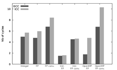
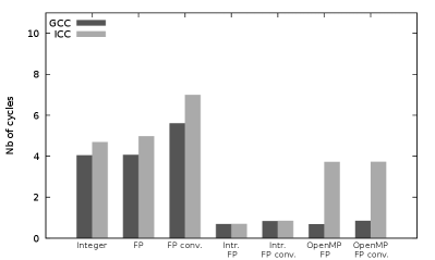
We start with microbenchmarks, presented in Fig. 1, of the two modular arithmetic operations and . Like all following performance tests, these microbenchmarks have been performed on the two compute servers AVX2 server and AVX-512 server presented in Table 1. We first notice that, regarding the original implementation of the modular multiplication (integer based, by R. Pearce), our microbenchmark results are consistent with the 6.016 cycles obtained with GCC by Monagan and coworkers[30] on older CPUs.
Regarding (see Figs. 1(a) and 1(b)), and with respect to the original integer based implementation, the scalar floating-point (FP) based implementation offers lower performance when including back and forth conversions between integers and floating-points numbers, and similar performance when not considering these conversions. The SIMD FP based implementation offer (with intrinsics, and without considering the conversions) a 3.2x (resp. 3.7x) speedup with GCC (resp. ICC) over the scalar FP-based implementation on AVX2 server. On AVX-512 server, the speedup is 5.9x (resp. 7.2x) speedup with GCC (resp. ICC). This shows that the performance gain of our new AVX-512 implementations is indeed twice greater than the AVX2 one.
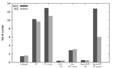
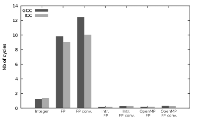
Regarding (see Figs. 1(c) and 1(d)), the scalar FP-based implementation leads to much greater cycle numbers than the integer-based one: this is due to the branching of the compare instruction required in the FP implementation (see Algorithm 3). The comparison in the integer-based implementation can indeed be replaced by shifting[34, 14], which avoids the branching performance impact on the pipeline filling. Thanks to the use of the AVX2 blendv_pd intrinsic and of AVX-512 masks, there is also no branching in the SIMD FP-based implementations (with intrinsics) which implies a strong performance gain (around one order of magnitude), in addition to the SIMD speedup. With respect to the scalar integer-based one, the SIMD speedups of the FP-based implementations with intrinsics (without considering the conversions) are 4.0x (resp. 3.6x) with GCC (resp. ICC) on AVX2 server, and 8.7x (resp. 8.5x) with GCC (resp. ICC) on AVX-512 server. This shows that our AVX-512 implementation is twice faster than the AVX2 one of Van der Hoeven et al.[14].
When considering the conversions, the overhead of these conversions can annihilate the SIMD performance gain on AVX2 server. This is due to the lack of AVX2 conversion instruction between 64-bit integers and 64-bit floating-point numbers: the conversions are thus performed in scalar mode which has a strong performance impact. In comparison, such a SIMD instruction is available in AVX-512333More precisely, the 64-bit conversions belong to the AVX-512DQ instruction set which is available on our Intel Xeon Gold 6152 CPUs, but not on the prior Intel Knights Landing (Xeon Phi) processors. , where conversions can be performed in SIMD mode. Their overheard is therefore much lower on AVX-512 server.
Finally, we also consider using OpenMP to vectorize the code.
The first issue lies in having the compiler generate SIMD FMA instructions
from the fma() function call in the C+OpenMP code for .
This is
effective with GCC thanks to the -fno-trapping-math option
which allows us to assume that floating-point operations cannot generate
traps, such as division by zero, overflow, underflow, inexact result and
invalid operation. Unfortunately, using all possible floating-point
model variations (-fp-model options) did not enable us to
generate SIMD FMA instructions with ICC. The ICC OpenMP code hence
relies on scalar FMA instructions, which explains its important
performance overhead over the GCC OpenMP code for .
Secondly, on AVX-512 server we had to force the AVX-512 vectorization using
-qopt-zmm-usage=high with ICC and
-mprefer-vector-width=512 with GCC, otherwise only AVX2
instructions are generated.
As far as is concerned, the OpenMP code (with GCC) has the same performance than the SIMD code written in intrinsics on AVX-512 server, but is slower by 18% on AVX2 server. This is because of one additional compare instruction added by the compiler before each blendv_pd instruction. This comparison to zero (either , or ) is here to prevent any issue with IEEE 754 signed zeros and the blendv_pd instruction. The compiler is indeed unaware of our specific context which enables us not to consider , as shown in Sect. 3.3.
For , the compiler similarly adds one unnecessary compare instruction which results in a 45% performance penalty on AVX2 server for the OpenMP code (with GCC). However no branching instruction is generated in the SIMD code for with OpenMP, which makes this OpenMP still rather efficient with respect to the scalar integer-based implementation: 2.8x faster on AVX2 server, and 7.4x on AVX-512 server (with GCC).
3.5 Integration in polynomial evaluation


We can now consider the integration of SIMD modular arithmetic in our partial polynomial evaluation. Due to the cost of the conversions between integers and floating-points numbers (see Sect. 3.4), we choose to perform the first conversion (from integers to floating-point numbers) for each value of the and vectors once before the evaluation (i.e. just before Line 1 in Algorithm 1). These conversions are performed in-place to save memory. The reverse conversion (from floating-point numbers to integers) is only performed once for each reduction result (i.e. the value at Line 10 in Algorithm 1).
Figure 2 presents performance results for our polynomial evaluation using various modular arithmetic implementations. One can see that the scalar floating-point based modular arithmetic makes our polynomial evaluation about 2.5 times slower than the original implementation by Monagan and coworkers[5] (using integer-based modular arithmetic). This is due to the slow FP-based implementation (because of its branch instruction: see Sect. 3.4).
We now consider SIMD intrinsics to integrate SIMD FP-based modular arithmetic in our originally scalar polynomial evaluation (see Algorithm 1). The resulting SIMD algorithm is written in Algorithm 6. First, a reduction has to be computed within the SIMD vector at the end of the inner loop (Line 14 in Algorithm 6), in order to obtain the final scalar value. Instead of performing a sequential reduction with the scalar and its branch instruction, we use SIMD shuffle instructions to write a parallel tree-shaped reduction using only SIMD operations. Second, we also have to consider memory alignement which can be important for efficient vector loads and stores. However, the indices used in the inner loop (Line 7 in Algorithm 6) do not lead to aligned memory accesses since the successive values are not necessarily multiples of the SIMD width. One could choose to make a copy of the vectors and with relevant zero padding to ensure aligned memory accesses, but this would require twice the memory. In order to obtain good SIMD speedups without padding, we explicitly decompose this inner loop into three successive loops , and (not shown in Algorithm 6). and have an iteration count lower than the SIMD width and are vectorized thanks to explicit masks. These two loops ensure that the vectorized loop perform aligned memory accesses (i.e. its first index is a multiple of the SIMD width). We noticed that the use of such a vectorized reduction and of such vectorized and loops offer additionnal performance gains when processing a lower number of terms: e.g. up to 29% for terms. With respect to the original implementation using integer-based arithmetic, the resulting polynomial evaluation with SIMD intrinsics offers performance gains ranging from 3.13x (resp. 3.89x) with GCC (resp. ICC) on AVX2 server to 4.18x (resp. 4.74x) with GCC (resp. ICC) on AVX-512 server (see Fig. 2).
Finally, we also consider using OpenMP vectorization for
the SIMD FP-based modular arithmetic in our
polynomial evaluation.
We rely on the
new declare reduction directive (available
since OpenMP 4.0) to instruct the compiler that
the final reduction (Line 14
in Algorithm 6) has to be performed
using our modular arithmetic.
We emphasize that the vectorization is achieved here thanks to
this OpenMP directive (along with the directive which
instructs the compiler to vectorize the loop with a reduction).
Without such directives given by the
programmer, the GCC and ICC compilers both manage to vectorize
the microbenchmarks presented in Sect. 3.4
(with the
same performance as the OpenMP version),
but both fail to vectorize the polynomial evaluation code
(because of the required specific reductions).
As shown in Fig. 2, the ICC OpenMP
vectorization is inefficient due to the FMA issue (see Sect.
3.4),
whereas the GCC OpenMP
vectorization offers computation times somewhat slower than the
intrinsic vectorization: 22% slower on AVX2 server, and 8% on AVX-512 server.
It can also be noticed that GCC currently fails to generate
align memory accesses (despite the use of the aligned
OpenMP clause) and SIMD reductions, as we do with intrinsics.
In conclusion, while the use of scalar FP-based modular arithmetic lowers the performance of the polynomial evaluation, the SIMD FP-based modular arithmetic clearly improves its performance (up to 4.74x). In the rest of the article, we will rely on the SIMD implementation with intrinsics, and not on the OpenMP one. This is due to the OpenMP performance issue with ICC and to the somewhat lower performance of the SIMD code generated with OpenMP, especially on AVX2 which still equips the vast majority of available CPUs at the time of writing. We however emphasize that the performance results of OpenMP with GCC on AVX-512 are very promising for the future and show the relevance of this approach.
As a last remark, we recall that regarding the microbenchmarks presented in Sect. 3.3 the AVX-512 and implementations are twice as fast than the AVX2 ones. Here however for the polynomial evaluation, the AVX-512 performance is only 1.57x (resp. 1.47x) faster than the AVX2 one with GCC (resp. ICC). We believe that this is due to the difference in operational intensities. Indeed, the microbenchmarks performed in Sect. 3.3 have been intentionally designed to be compute-bound in order to measure the number of cycles of the arithmetic operations, and not of the memory accesses. But the operational intensity of our polynomial evaluation is much lower: the Hadamard product and the coefficient reduction correspond to a dot product which is a memory-bound operation in classic floating-point arithmetic. More precisely, the floating-point based modular arithmetic requires 9 flop (floating-point operation) for (see Algorithm 2) and 2 flop for (see Algorithm 3), versus 3 memory accesses for each (2 loads and 1 store, without considering and ). This makes our compute kernel (i.e. our polynomial evaluation) less memory-bound than a floating-point dot-product, but the operational intensity of our kernel is not high enough to make it compute-bound: memory accesses are still important in the kernel performance. These memory accesses also tend to lower the performance gain due to the increased compute power of the AVX-512 SIMD units, with respect to the AVX2 units, since there is more stress on memory bandwidth with AVX-512 instructions than with AVX2 ones. We will show how to increase this operational intensity and the polynomial evaluation performance in the next section.
4 Increasing the compute efficiency
We now focus on the compute efficiency of our SIMD polynomial evaluation. More precisely, we aim to fill at best the pipelined floating-point units and to minimize the time lost in memory accesses.
4.1 Multiple dependent evaluations
We first rely on the consecutive powers of used for the successive evaluations in the matrix method (see Sect. 2.3). Hence in Algorithm 6, if we consider two consecutive polynomial evaluations and , the values computed in the vector for the evaluation are re-used as input for evaluation . But for large values ( denoting the number of terms, see Sect. 2.3), the elements may have been moved out of the CPU caches. We hence consider computing multiple evaluations at a time, and we denote by the number of such (dependent) evaluations. is an algorithmic constant, known at compile time. We can then explicitly avoid storing and reloading data from the vector to/from memory between these evaluations. We can also load only once data from memory for these evaluations. Such data reuse increases the operational intensity of our kernel by reducing the number of memory accesses.
However each evaluation depends on the output of the previous one. Even if some operations can be performed concurrently (such as the operation of the evaluation and the of the evaluation), this dependency limits the instruction-level parallelism, and hence prevents us from filling the pipelines of the floating-point units.
4.2 Multiple independent evaluations
Therefore, we rewrite the loop over the evaluations (Line 1 in Algorithm 1) in order to have fully independent polynomial evaluations. For this purpose, we adapt the algorithm used by Hu and Monagan[5] to introduce thread-level parallelism on multi-core CPUs (see Sect. 2.3.1) in order to introduce here instruction-level parallelism in our compute kernel. Namely, denoting by the desired number of independent evaluations (like , is an algorithmic constant, known at compile time), we first precompute using SIMD multiplications. We also precompute for using SIMD multiplications. Then, for the computation of the evaluations we will first perform the coefficient reductions for the first evaluations (i.e. on ), then the Hadamard product (with ) for the second chunk of evaluations. This will be repeated (coefficient reductions on the previous evaluations, then Hadamard product for the next evaluations) until all evaluations have been processed.
This instruction-level parallelism helps fill the instruction pipelines. Moreover the and operations are now inverted. Contrary to Algorithm 1 (Lines 7-8) where the second operation depends on the output of the first one, the second operation now only depends on the input of the first one. The two operations can thus be more overlapped, hence easing the pipeline filling.
The main drawback of using independent evaluations is the extra memory requirements. For each independent evaluation we have to store an extra copy of the complete vector. Moreover, for each independent evaluation we have to load the vector from memory and store its update in memory. The operational intensity is thus only improved for the memory accesses. Therefore, introducing an extra independent evaluation increases less the operational intensity than introducing an extra dependent evaluation.
There is hence a trade-off between pipeline filling and operational intensity regarding the numbers of dependent () and independent () evaluations. We will thus consider an algorithm where we introduce dependent evaluations for each of the evaluations, hence computing together evaluations at a time. The loop over is chosen as the outer one, and the loop over as the inner one: this results in better performance than the opposite loop ordering, which indicates that pipeline filling is here more important than increasing the operational intensity. The optimal values for and depend on the compiler and on the CPU hardware features, and these will have to be determined in practice using parameter testing and tuning. Since the total number of evaluations is not necessarily a multiple of , the remaining evaluations are processed first by blocks of evaluations (with ) and then with dependent evaluations (with ), where .
| … | … | ||||
| … | … | ||||
| … | … | ||||
| … | … |
| … | … | ||||
|---|---|---|---|---|---|
| … | … | ||||
| … | … | ||||
| … | … | ||||
| … | … | ||||
| … | … |
| … | … | … | |||||
|---|---|---|---|---|---|---|---|
| … | … | … | |||||
| … | … | … | |||||
| … | … | … | |||||
| … | … | … | |||||
| … | … | … |
| … | … | ||||
|---|---|---|---|---|---|
| … | … | ||||
| … | … | ||||
| … | … | ||||
| … | … | ||||
| … | … |
The final version is presented in Algorithm 7, along with the SIMD programming. Once evaluations have been computed together for some monomials, we could choose to iterate over the next evaluations or to iterate over the next monomials with same values. If we had iterated over the next evaluations, we would have had to store SIMD vectors (all () for the coefficient reductions. By iterating on the next monomials (as done in Algorithm 7), SIMD loads (all and for ) and SIMD stores (all ) are required. As in practice (as confirmed for the optimal configurations in Sect. 4.4), it is indeed preferable to iterate over the next monomials in order to minimize the number of memory accesses and hence increase the operational intensity. This results in the end in an algorithm where we browse all the monomials with same values to compute evaluations at a time. An illustration of the execution of Algorithm 7 is given in Fig. 3.
4.3 Loop unrolling
Loop unrolling[6] enables us to remove the exit test at the end of the loop body and to interleave instructions from successive loop iterations in order to better fill the pipelines. The two nested loops over the and evaluations (Lines 11 and 12 in Algorithm 7) are hence completely unrolled thanks to the “unroll(F)” pragma of ICC and to the “GCC unroll F” pragma of GCC (recently introduced in GCC 8) to impose an unroll factor of F (F being respectively equal to and ). Similarly, we unroll the third loop over the monomials with same values (Line 8 in Algorithm 7) by a factor . We could also have let the compiler choose which loops to unroll (or not) and determine the best unroll factors. This leads to similar performance with GCC, but to lower performance with ICC (up to 8.5% performance loss). We thus impose our unrollings on the three loops with the corresponding pragmas.
Once the three nested loops have been unrolled, we rely on the compiler and on the out-of-order execution of the processor to schedule at best the instructions to fill the pipelines and to overlap the memory accesses. Other loops over and/or evaluations (Lines 9, 17, 19, 20, in Algorithm 7) are also similarly unrolled.
4.4 Performance results
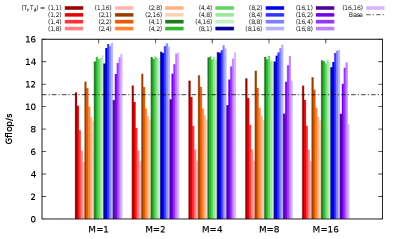
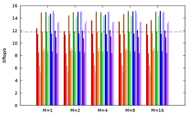
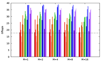

Using the test platforms (server and compiler) described in Table 1, we present in Figure 4 the performance results for all possible configurations for (, , ), each value ranging in 1,2,4,8,16. We also indicate the performance of the Base SIMD code corresponding to the version obtained with the SIMD intrinsics only (as presented in Sect. 3). The performance varies significantly depending on the (, , ) values, especially on and , which shows the relevance of these parameters. The performance impact of is lower but can still reach 11% for some (, ) configurations. The best configurations are the following.
-
•
(, , ) with GCC on AVX2 server: 15.65 Gflop/s, and 42% of performance gain over the Base SIMD code.
-
•
(, , ) with ICC on AVX2 server: 15.21 Gflop/s, and 29% of performance gain over the Base SIMD code.
-
•
(, , ) with GCC on AVX-512 server: 39.11 Gflop/s, and 121% of performance gain over the Base SIMD code.
-
•
(, , ) with ICC on AVX-512 server: 37.31 Gflop/s, and 109% of performance gain over the Base SIMD code.
As determining the theoretical peak performance of modern CPUs becomes more and more complicated[35], we use the BLAS DGEMM routine of the Intel MKL444See: https://software.intel.com/en-us/mkl to estimate the single-core double-precision peak performance at 45 Gflop/s on AVX2 server and 101 Gflop/s on AVX-512 server. Moreover, we can only reach 61% of the peak performance since there are only 2 FMAs out of the 9 floating-point instructions required for and . We manage hence to reach 57% and 63% of the attainable single-core peak performance, respectively on AVX2 server and on AVX-512 server.
| Server | Compiler | Reference scalar integer-based version (time in ms) | SIMD FP-based version with improved compute efficiency (time in ms) | Gain |
| AVX2 server | GCC | 15262 | 3482 | 4.4x |
| AVX2 server | ICC | 17704 | 3671 | 4.8x |
| AVX-512 server | GCC | 12984 | 1411 | 9.2x |
| AVX-512 server | ICC | 14638 | 1476 | 9.9x |
In the end, as shown in Table 2, we manage to reach speedups of almost 5x and 10x (respectively on AVX2 server and on AVX-512 server) on one CPU core over the reference original polynomial evaluation with scalar integer-based modular arithmetic. It can be noticed that Monagan and coworkers already used to process two (dependent) evaluations at a time to increase the operational intensity for some variants of the polynomial evaluation. However for the variant studied in this article (see Algorithm 1), which is the fastest one, no performance gain is obtained by processing two evaluations at a time with the original scalar code. Such divergence with respect to the gains obtained in Fig. 4 can be explained by the lack of other optimizations (multiple independent evaluations, loop unrollings) as well as by the differences in the modular arithmetic implementation between the original integer-based version by Monagan and coworkers and the floating-point based version of this article.
4.5 Without extra memory requirements
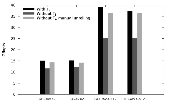
One drawback of using multiple independent evaluations is the significant memory overhead: the complete vector has to be duplicated for each extra independent evaluation. We therefore investigate here the best attainable performance without any extra independent evalution.
We first implement a code without multiple independent evaluation, and tune the and parameters for this code via extensive benchmarks (as in Sect. 4.4). Figure 5 shows for each test platform the performance drop obtained for this code (referred to as Without ) with respect to the best version obtained in Sect. 4.4 (referred to as With ). The performance drop is important here (up to 36%), due to the lower number of independent instructions to fill the pipelines.
We then introduced manual loop unrolling, using preprocessor macros to ease and automate the tedious code writing. We also manually group all arithmetic instructions. This way, we provide all arithmetic instructions for the computation of dependent evaluations and monomials to the compiler and to the out-of-order execution of the processor, so that these can be scheduled at best to fill the pipelines. One can see that this new version (referred to as: Without , manual unrolling; and after tuning of its and parameters) greatly reduces the performance drop with respect to the best version obtained in Sect. 4.4 (With ). This way, we can reach 95% (GCC) and 94% (ICC) on AVX2 server and 93% (GCC) and 98% (ICC) on AVX-512 server of the best attainable performance (With ). At the price of non-negligeable development efforts, we can thus obtain, without introducing extra memory, almost the same performance of our best versions with multiple independent evaluations.
It can also be noticed that the performance impact of is here much more important than in Sect. 4.4 (detailed tests not shown). Such manual loop unrolling and instruction grouping have also been tried on the best version obtained in Sect. 4.4 (with multiple independent evaluations): this however only offers up to 5.1% performance gain for such code. In our opinion, this does not justify the manual unrolling development effort when using multiple independent evaluations.
5 Conclusion
In this article, we have first justified the choice of a modular multiplication algorithm relevant for HPC and SIMD computing. We have ensured the correct use of an optimized AVX2 implementation (regarding a potential issue with signed zeros and the blendv_pd intrinsic) and we have presented its AVX-512 version. This floating-point (FP) based algorithm with FMAs (fused multiply-adds) enables us to obtain SIMD speedups of up to 3.7x on AVX2, and up to 7.2x on AVX-512, which validates its efficiency. With respect to a reference (scalar) integer-based modular arithmetic, the performance gains are similar for our SIMD FP-based modular multiplication and for the corresponding SIMD FP-based modular addition. As all current desktop and HPC processors have SIMD units, we believe that such SIMD FP-based modular arithmetic should from now on be used instead of the scalar ones. Using OpenMP for their SIMD programming turned out to be a very promising approach on the new AVX-512 units (with GCC), due to its very relevant performance-programmability trade-off. Currently, we still rely on intrinsics programming for best performance and performance portability among compilers.
In a second part, we have focused on the partial polynomial evaluation which is a key computation in Computer Algebra. We have rewritten this algorithm in order to introduce multiple independent and dependent evaluations. These enable us, along with loop unrolling, to fill at best the pipelined floating-point units of the CPU and to minimize the time lost in memory accesses. Combined with SIMD computing, we achieve speedups up to almost 5x on AVX2 and up to almost 10x on AVX-512 with respect to the reference implementation of the polynomial evaluation. Moreover, using manual loop unrolling we manage to closely reach such performance gains without extra memory requirements.
In the future, we plan to integrate our efficient polynomial evaluation on one CPU core in the multi-core parallel implementation of Monagan and coworkers[5, 17], and to study the performance impact on polynomial factorizations and polynomial greatest common divisor computations. We also believe that GPUs may be well suited to further accelerate our polynomial evaluation thanks to their higher compute power and memory bandwidth. We emphasize that our FP-based modular arithmetic will be very relevant for the GPU FMA SIMD units, and will offer a direct and efficient implementation of modular arithmetic on GPUs. We may also investigate using a few less bits for our prime in order to decrease the number of reductions as done for example with error-free transformations in linear algebra[36].
Acknowledgments
The authors would like to thank the master in computer science at Sorbonne Université, especially N. Picot and P. Cadinot, for administering and providing access to the compute servers. They also thank Professor S. Graillat (Sorbonne Université) for helpful discussions on error-free transformations.
References
- [1] Donald E. Knuth. The Art of Computer Programming, Volume 2 (3rd Ed.): Seminumerical Algorithms. Addison-Wesley, Boston, MA, USA, 1997.
- [2] Keith O. Geddes, Stephen R. Czapor, and George Labahn. Algorithms for Computer Algebra. Springer, 1992.
- [3] Joachim Von Zur Gathen and Jurgen Gerhard. Modern Computer Algebra. Cambridge University Press, USA, 2 edition, 2003.
- [4] Michael Monagan and Baris Tuncer. The complexity of sparse Hensel lifting and sparse polynomial factorization. Journal of Symbolic Computation, 99:189 – 230, 2020.
- [5] Jiaxiong Hu and Michael Monagan. A Fast Parallel Sparse Polynomial GCD Algorithm. Proceedings of the ACM on International Symposium on Symbolic and Algebraic Computation, pages 271–278, New York, NY, USA, 2016. ACM.
- [6] J.L. Hennessy and D.A. Patterson. Computer Architecture: A Quantitative Approach, Sixth Edition. The Morgan Kaufmann Series in Computer Architecture and Design, 2017.
- [7] Samuel Williams, Andrew Waterman, and David Patterson. Roofline: An insightful visual performance model for multicore architectures. Commun. ACM, 52(4):65–76, April 2009.
- [8] Intel Developer Services. MMX Technology Technical Overview, 1996.
- [9] AMD. 3DNow! Technology Manual, 2000.
- [10] Intel. Intel SSE4 Programming Reference, Reference number: D91561-003, 2007.
- [11] K. Diefendorf. Altivec extension to Power PC accelerates media processing, 2001.
- [12] Intel. Intel Architecture Instruction Set Extensions Programming Reference, Number: 319433-012A, 2012.
- [13] Intel. Intel Architecture Instruction Set Extensions Programming Reference, Number: 319433-024, 2016.
- [14] Joris Van Der Hoeven, Grégoire Lecerf, and Guillaume Quintin. Modular SIMD arithmetic in Mathemagix. ACM Trans. Math. Softw., 43(1):5:1–5:37, August 2016.
- [15] Richard E. Zippel. Probabilistic algorithms for sparse polynomials. Symbolic and Algebraic Computation, EUROSAM ’79, pages 72:216–226, Berlin, Heidelberg, 1979. Springer.
- [16] Richard E. Zippel. Interpolating polynomials from their values. Journal of Symbolic Computation, 9(3):375 – 403, 1990.
- [17] Michael Monagan and Baris Tuncer. Sparse multivariate polynomial factorization: a high-performance design and implementation. Mathematical Software – ICMS 2018, pages 359–368, Cham, 2018. Springer International Publishing.
- [18] Michael Ben-Or and Prasoon Tiwari. A deterministic algorithm for sparse multivariate polynomial interpolation. In Proceedings of the Twentieth Annual ACM Symposium on Theory of Computing, STOC ’88, pages 301–309, New York, NY, USA, 1988. Association for Computing Machinery.
- [19] Daniel S. Roche. What can (and can’t) we do with sparse polynomials? In Proceedings of the 2018 ACM International Symposium on Symbolic and Algebraic Computation, ISSAC ’18, pages 25–30, New York, NY, USA, 2018. ACM.
- [20] Jiaxiong Hu and Michael Monagan. A fast parallel sparse polynomial GCD algorithm. Journal of Symbolic Computation, 2019 (submitted).
- [21] Joris Van Der Hoeven and GréGoire Lecerf. On the Bit-complexity of Sparse Polynomial and Series Multiplication. Journal of Symbolic Computation, 50:227–254, March 2013.
- [22] Michael Monagan and Alan Wong. Fast Parallel Multi-point Evaluation of Sparse Polynomials. Proceedings of the International Workshop on Parallel Symbolic Computation, pages 4:1–4:7, New York, NY, USA, July 2017. ACM.
- [23] Agner Fog. Optimizing software in c++. an optimization guide for windows, linux and mac platforms. Technical report, Technical University of Denmark, 2018. https://www.agner.org/optimize/.
- [24] R. Alverson. Integer division using reciprocals. Proceedings 10th IEEE Symposium on Computer Arithmetic, pages 186–190, June 1991.
- [25] Henry G. Baker. Computing a*b (mod n) efficiently in ansi c. SIGPLAN Not., 27(1):95–98, January 1992.
- [26] Paul Barrett. Implementing the rivest shamir and adleman public key encryption algorithm on a standard digital signal processor. Advances in Cryptology — CRYPTO’ 86, pages 311–323, Berlin, Heidelberg, 1987. Springer Berlin Heidelberg.
- [27] Torbjörn Granlund and Peter L. Montgomery. Division by invariant integers using multiplication. Proceedings of the ACM SIGPLAN 1994 Conference on Programming Language Design and Implementation, pages 61–72, New York, NY, USA, 1994. ACM.
- [28] Peter L. Montgomery. Modular multiplication without trial division. Mathematics of Computation, 44(170):519–521, 1985.
- [29] N. Moller and T. Granlund. Improved division by invariant integers. IEEE Transactions on Computers, 60(2):165–175, Feb 2011.
- [30] Matthew Gibson and Michael Monagan. Optimizing and Parallelizing the Modular GCD Algorithm. In Proceedings of the 2015 International Workshop on Parallel Symbolic Computation, PASCO ’15, pages 44–52, New York, NY, USA, 2015. ACM.
- [31] Takeshi Ogita, Siegfried M. Rump, and Shin’ichi Oishi. Accurate sum and dot product. SIAM J. Sci. Comput., 26(6):1955–1988, June 2005.
- [32] IEEE Standard for Floating-Point Arithmetic. IEEE Std 754-2008, pages 1–70, Aug 2008.
- [33] Gabriell Orisaka, Julio López, and Diego F. Aranha. Finite field arithmetic using avx-512 for isogeny-based cryptography. XVIII Simpósio Brasileiro de Segurança da Informação e Sistemas Computacionais (SBSeg 2018), pages 49–56, 2018.
- [34] Marshall Law and Michael Monagan. A parallel implementation for polynomial multiplication modulo a prime. Proceedings of the 2015 International Workshop on Parallel Symbolic Computation, pages 78–86, New York, NY, USA, 2015. ACM.
- [35] Romain Dolbeau. Theoretical peak FLOPS per instruction set: a tutorial. The Journal of Supercomputing, 74(3):1341–1377, Mar 2018.
- [36] J. Jean and S. Graillat. A parallel algorithm for dot product over word-size finite field using floating-point arithmetic. 12th International Symposium on Symbolic and Numeric Algorithms for Scientific Computing, pages 80–87, 2010.