High Performance Distributed Control Law for Large-Scale Linear Systems: A Partitioned Distributed Observer Approach
Abstract
In recent years, the distributed-observer-based distributed control law has shown powerful ability to arbitrarily approximate the centralized control performance. However, the traditional distributed observer requires each local observer to reconstruct the state information of the whole system, which is unrealistic for large-scale scenarios. To fill this gap, this paper develops a greedy-idea-based large-scale system partition algorithm, which can significantly reduce the dimension of local observers. Then, the partitioned distributed observer for large-scale systems is proposed to overcome the problem that the system dynamics are difficult to estimate due to the coupling between partitions. Furthermore, the two-layer Lyapunov analysis method is adopted and the dynamic transformation lemma of compact errors is proved, which solves the problem of analyzing stability of the error dynamic of the partitioned distributed observer. Finally, it is proved that the distributed control law based on the partitioned distributed observer can also arbitrarily approximate the control performance of the centralized control law, and the dimension of the local observer is greatly reduced compared with the traditional method. The simulation results show that when the similarity between the physical network and the communication network is about , the local observer dimension is greatly reduced by and the relative error between the performance of the distributed control law and that of the centralized control law is less than .
Index Terms:
Distributed observer, Continuous time system estimation, Consensus, Sensor networks, Switching topologiesI Introduction
Distributed observer is a cooperative observer network composed of agents and a communication network. Each agent is a node of the network and contains a local observer as well as a local controller. Each local observer only has access to partial system outputs, and all local observers cooperate to complete the state estimation of the whole system through information interaction via communication networks. Distributed observer has extensive application value and profound theoretical value. In terms of application value, global scholars have enabled distributed observer to play important roles in flexible structures [1], smart vehicles [2], microgrids [3, 4], deep-sea detectors [5, 6], spacecraft in low Earth orbit [7] and other fields. In terms of theoretical value, distributed observer can help distributed control law to improve its performance with a qualitative change. Readers may refer the theoretical value to the article of [2, 8, 9], [10], and [11], which prove that the distributed-observer-based distributed control law has the same performance as that of the centralized control law. Owing to its broad application prospects and outstanding theoretical significance, distributed observer finds itself a center of research in recent years [12, 13, 14, 15, 16, 17, 18, 19, 20, 21, 22, 24, 25, 26].
It should be noted that the current distributed observer has an obvious shortage: It requires that every agent has to reconstruct the states of the whole system. In other words, if the system dimension is , then the dimensions of local observers on every agent are all , which is the origin of a special term in the field of distributed observer: state omniscience. Accordingly, it is barely able for a large-scale system to achieve state omniscience because of the high dimensions of local observers. After all, we cannot require each agent to compute a local observer with the same dimension as the large-scale system, otherwise, we will lose the original intention of the distributed design. Although a few articles have studied the minimum order distributed observer [28] or reduced order distributed observer [29], they replace full-dimension observers contained in the local observer with reduced-dimension observers. It cannot essentially solve the problem of the high dimension of local observers caused by large-scale systems.
This paper will explore whether there is a method that can effectively reduce the dimension of local observers on each agent. One of the biggest challenges in studying this problem is to reduce the dimension of local observers without affecting their ability to help distributed control approach centralized control performance. According to [30], we know that the reason why distributed control law cannot achieve the same performance as that of the centralized control law is that distributed control law cannot obtain as much state information as centralized control. However, in [2], an agent can estimate the whole system states through the state omniscience of distributed observer. It indicates that state omniscience is an important factor in why the distributed-observer-based distributed control law has centralized control performance. Therefore, approaching the centralized control performance without relying on state omniscience presents the distributed-observer-based distributed control law with huge challenges.
The idea to overcome these challenges in this paper comes from the thinking of large-scale interconnected systems structure. We find that, for large-scale interconnected systems (it is better to use a graph to represent the interconnection relationship among subsystems and name this graph as the physical network), the local control law on each agent does not actually need the whole large-scale system states. Generally speaking, the states of physical network neighbor agents are enough for an agent to achieve centralized control performance. For example, the states employed in the centralized control law of interconnected microgrid systems are only the states of each agent’s physical network neighbor agents. Inspired by this, can we build a novel distributed observer so that the local observer on each agent only needs to estimate the states of its physical neighbor agents? If feasible, the local observer dimension on each agent can be greatly reduced because the interconnection of a large system is often sparse, and the average number of physical neighbor agents of each agent is generally far less than the number of all agents. In addition, since the states of all physical neighbor agents of an agent are estimated, the local control law can use the same state information as that of centralized control. It indicates that the aforementioned method does not affect the performance of the distributed observer and its role in distributed control law while reducing the dimension of all local observers.
Building the above-mentioned new distributed observer is a formidable task because a local observer containing only the physical network neighbor states can be established if and only if the physical network and communication network are identical. Unfortunately, physical networks and communication networks are generally different. For this reason, this paper tries to develop a method to partition all nodes. Each partition contains multiple nodes, and each node belongs to multiple partitions. Then, distributed observer can be designed in each partition, and all agents can complete the state estimation of all their physical neighbors through one or more partitioned distributed observers. Hence, the main focus of the partition is on enabling the union of all partitions on an agent to cover all its neighbor agents (this is a necessary condition to ensure that the distributed-observer-based distributed control law has centralized control performance), and also requiring the number of agents in the union of partitions to be as small as possible (reduce the dimension of local observers on each agent as much as possible).
Therefore, the first scientific challenge faced by this paper is how to establish an intelligent partition method that meets the above conditions. There is a lot of research on large-scale network partition in the existing literature, but these methods are based on one or more of the following conditions: 1) No intersection between any two partitions [31, 32, 33]; 2) One needs to know how many partitions in advance [34]; 3) There is a clear and single objective function [35, 33, 36]; 4) Partition the node coverage area [37, 38]. However, the partition problem in this paper does not meet any of the above conditions. Furthermore, the existing partition methods are all based on the topology information of only one network, while the topology information of two networks (physical network and communication network) should be considered at the same time in this paper. Therefore, the existing partition methods are not applicable to this work.
The second scientific challenge is how to deal with the problem of error dynamic coupling between various partitions. Although the idea of this paper is to partition large-scale systems and build distributed observer for small-scale systems within the partitions, distributed observers in the partitions are not independent, and they are dynamically coupled with the distributed observer in other partitions. If we do not eliminate this coupling, the observer is not implementable because they include the unknown states from other partitions. On the contrary, if this coupling is eliminated, we will face the model mismatch problem. What is more difficult is that even if the coupling relationship is eliminated in the observer design, it will occur in the error dynamics and lead to the difficulty of stability analysis. Therefore, the classical distributed observer theory, which is close to maturity, cannot be used either in the partitioned distributed observer design or in the error dynamic stability analysis.
Focusing on the above challenges, this paper contributes to the following three aspects:
1) We propose a reasonable and feasible partition method for large-scale systems. Furthermore, the partition method proposed in this paper can achieve the Pareto optimal solution (Each agent has its own most expected partitioning result, so the partitioning problem in this paper is a multi-objective optimization problem).
2) A design method is proposed for the partitioned distributed observer and a two-layer Lyapunov method is developed to analyze the stability of the error dynamic of the partitioned distributed observer. The proposed method guarantees the implementation of the partitioned distributed observer. It is also proved that each agent can estimate the states of all its physical network neighbor agents, and the estimation error can dynamically converge to any small invariant set.
3) Although the dimension of each local observer is greatly reduced, the distributed control law based on the partitioned distributed observer can still arbitrarily approximate the control performance of centralized control. It provides an important theoretical basis for the application of distributed observer in large-scale systems.
The remainder of this paper is organized as follows. Section II formulates the problem. Section III gives the partition method and partitioned distributed observer design method. The performance of the error dynamics of partitioned distributed observer and closed-loop system are analyzed in Section IV. The simulation results are given in Section V, and Section VI concludes this paper.
Notations: Let be the Euclidean space of -dimensional column vectors and be the Euclidean space of -dimensional matrices. Denote the transpose of matrix . and stand for the maximum and minimum eigenvalues of , respectively, if . We cast as , and as a block diagonal matrix with on its diagonal, where are matrices with arbitrary dimensions. represents the dimension of a vector. is an identity matrix and if is a square matrix. We denote the cardinality of a set. represents the -norm of vectors or matrices. Furthermore, there are many symbols in this paper. To avoid confusion for readers, we have listed a comparison table of easily confused symbols in Table 1, and corresponding symbols will also be explained when they first appear.
| Symbol | Definition |
|---|---|
| The th partition | |
| Set of partitions that containing node | |
| Estimation of generated by observers on agent in partition | |
| Saturate value of | |
II Problem formulation
II-A Overall objectives
Consider a large-scale interconnected system composed by subsystems (corresponding to agents) and the th subsystem takes the form of:
| (1) | |||
| (2) |
where , , and are the system states, output measurements, and control inputs of the th subsystem, respectively; is the state of the th subsystem; The matrices , , and represent the system matrix, control matrix, and output matrix of the th subsystem with compatible dimensions, respectively; and stands for the coupling matrix between the th and the th subsystems. Let , , and , then the compact form of the large-scale system is given by
| (3) | |||
| (4) |
where , , and .
We construct a physical network for this large-scale system by its interconnection. Let be the nodes (agents) set and we say is an edge connecting and if . Then, the set is defined by . Accordingly, the adjacency matrix is defined as where if . Let be the set of physical network neighbors of agent . The physical network can be directed or undirected and the schematic diagrams in this paper all use undirected graphs, but it should be noted that when the physical network is an undirected graph, the system matrix is assumed to have constraints with ; When the physical network is a directed graph, the system matrix has no constraints. Moreover, an undirected graph represents the communication network among all nodes, where and are the associated edge set and adjacency matrix, respectively. Then, the set of communication network neighbors of agent is given by . The Laplacian matrix associated to is denoted by , where with .
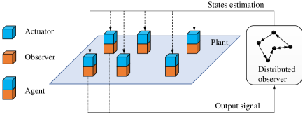
In traditional distributed observer, each local observer—the orange block in Figure 1—is required to reconstruct all the states of the entire system based on and the information exchanged via communication network. Then, each local controller—blue block in Figure 1—can use all the information of the entire system. Therefore, all local observers can jointly establish a distributed control law with centralized performance. Many existing studies, such as [2, 9], have proved this result, i.e., the distributed-observer-based distributed control law can achieve centralized control performance. However, in these studies, each local observer needs to reconstruct the states of the whole system, i.e, dimension of observers on each agent is . This is not realistic for large-scale systems. Therefore, this paper will investigate whether it is possible to achieve distributed control laws with arbitrary approximation of centralized control performance without requiring each local observer to estimate global information.
To formulate the problem, we assume that there is a centralized control law such that system (3) is stabilized, and denote the solution of (3) with centralized control law. We further assume a distributed control law such that solved by (3) with is stabilized, where is the states estimation generated by the th local observer located at the th agent, and . Subsequently, the overall goal of this paper consists of the following two parts.
1) Design the partitioned distributed observer with being the states of the th local observer, and satisfies ;
2) Design a distributed-observer-based distributed control law such that can approach arbitrarily, i.e., , and .
II-B An illustrative example for the target problem
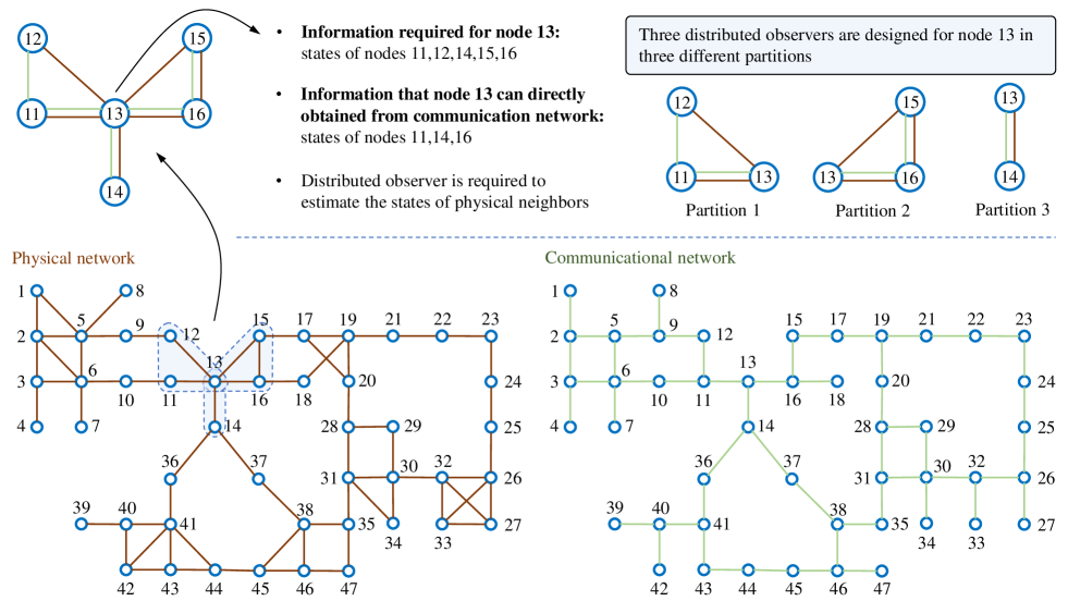
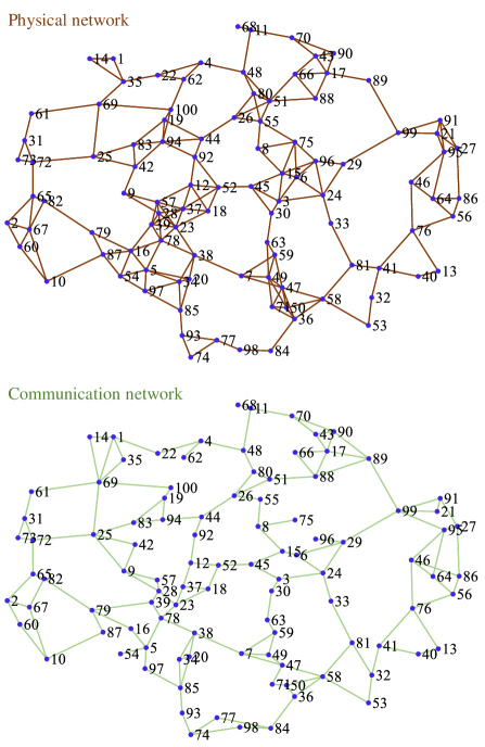
In this subsection, we will illustrate an example for helping readers understand the problems proposed in the above subsection. See in Figure 2, the coupling relationship of a large-scale system is shown in the physical network, in which each node represents an subsystem. Assume that each subsystem has a corresponding agent, and the communication relationship among all agents is shown as communication network. The th agent has access to the information of , and is supposed to establish several local observers and a local control law.
We take node as an example to demonstrate the specific issues to be studied in this paper. As seen in Figure 2, node has physical neighbors () and communication neighbors (). To design a local control law to make the control performance as close as possible to the centralized control law, agent needs the states of all its physical neighbors. In traditional method, a distributed observer will be designed such that agent can reconstruct all states of the entire system. However, only the states of are required. Therefore, this paper intends to design a group of partitions and design distributed observer in each partition. In this way, the useless information estimated by each agent can be greatly reduced. For example, in Figure 2, node belongs to partitions—, , and . By designing distributed observers separately in three partitions, agent only needs to estimate the states of subsystems (in traditional methods, agent needs to estimate the states of all subsystems). With partitioned distributed observers, local control laws can be established based on the results of state estimation.
Up to now, we have briefly described the main idea of this paper through an example. To achieve this idea, there are mainly three steps involved: 1) Design a reasonable and effective partitioning algorithm; 2) Design partitioned distributed observer in each partition; 3) Design distributed control law.
Before achieving these steps, we first specify two basic assumptions and an important lemma.
Assumption 1
Pair is assumed to be controllable and for are assumed to be observable.
Assumption 2
Graphs corresponding to communication network is assumed to be undirected, connected and simple (A graph or network is simple means there is no self-loop and multiple edges).
Lemma 1 ([39])
Consider an undirected connected graph . Let and then all eigenvalues of matrix locate at the open right half of plane, where is the Laplacian matrix of .
Remark 1
The reader should note that Assumption 1 is not completely the same as the traditional assumption in distributed observers. In existing literature [15, 9], it is generally assumed that is observable, but may not be observable. Assumption 1 used in this paper is given owing to the form of system (1)–(2). This system format is easier to express our core views on partitioning and status information retrieval. Actually, the partitioned distributed observer can also be achieved based on the General system and the traditional assumption as in [15, 9]. However, due to limitations in space and the need to express the main idea, the theory of partitioned distributed observers for general systems will be included in our future research.
III Design of partitioned distributed observer
A large-scale network partition algorithm will be given in this section. Then, based on the partition results, we propose the design method and observer structure of the partitioned distributed observer.
III-A Network partition
As mentioned in Section I and Subsection II-B, it is unnecessary to require each local observer to reconstruct the states of the whole large-scale system. Theoretically, each agent only needs to estimate part of states required by its local control law. Therefore, in order to establish a distributed observer that can only estimate the state information required by the local control law, we need to partition the network and ensure that all partitions of each agent contain all its physical network neighbors. To illustrate it in more detail, we introduce several simple examples.
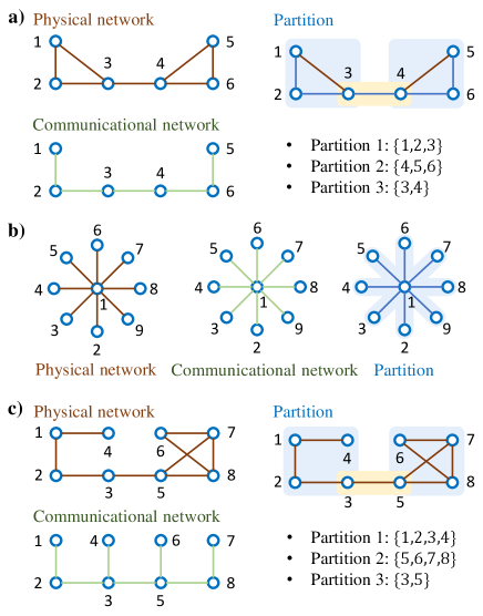
In Figure 3a), there is a simple network system with nodes. One may recognize its partition by observation easily: it could be partitioned into three categories with , and . With this partition, the physical network neighbors of all nodes have been included in their partitions. For example, , and partitions to which node belonging are and . Obviously, . Similarly, Figure 3b) is a star network system with nodes. One can partition it with , , , , , , , and all agents’ physical neighbors are covered by their partitions. As for Figure 3c), the acquisition of partitions is not so intuitive, but we can still partition it with , , and after the observation and analysis. Through the above examples, we know the basic idea and function of partition, but we cannot obtain reasonable partition results through observation for large-scale systems. Therefore, a reasonable partition algorithm is necessary for distributed observers of large-scale systems.
To this end, we propose a partition method based on the greedy algorithm. Before showing the algorithm details, some notations are introduced. is defined as the th partition of the large-scale system, and denotes the set of partitions that containing node . For example, in Figure 3c), , , and . In addition, , and . Set , and denote the total number of agents that need to be estimated by local observer on the th agent. Let be a set of the nodes belonging to the shortest path between and in communication network . For example, in Figure 3c), . Besides, we define for nodes belonging to , and define the symbol by if , or and . In addition, define for nodes belonging to , and further define by if , or and .
Now, one can see Algorithm 1 for the developed partition method. For the convenience of readers to understand the algorithm, we will briefly describe the algorithm process here.
Step 1: Sort based on symbol .
Step 2: Starting from the minimum . Each node chooses its partitions according to the greedy algorithm in sequence (The larger the degree of node in the communication network, the more partition schemes can be selected. Therefore, priority should be given to the node with the smallest communication network degree).
Step 3: Sort based on symbol .
Step 4: Starting from the maximum . Each node considers whether to merge several partitions according to two criteria (Line 27–29 in Algorithm 1 and their details are shown in (D2)) in sequence (In communication networks, nodes with larger degrees are more likely to be forced to join many redundant partitions. Therefore, priority is given to nodes with larger degrees to determine whether to remove some redundant partitions through merging).
Note that the partition algorithms described in Algorithm 1 and Algorithm 2 actually solve a multi-objective optimization problem because each node has its own desired partition result, but the desired optimal partitions among different nodes are conflicting. In the complete version of this article, we prove that the partition results obtained through Algorithm 1 and Algorithm 2 are Pareto solutions to this multi-objective optimization problem.
Propsition 1
Proof:
Given a group of partitions () obtained by Algorithm 1 and Algorithm 2. We first prove three propositions.
1) Add any nodes in arbitrary would increase the dimensions of observers on at least one node. Since is obtained by at least one node (denote as ) within the partition using a greedy algorithm, node makes the optimal choice when selecting based on the current situation. Now, let’s discuss two scenarios. First, has yet to be included in any partition before selecting . In this case, is the first partition for , so it is the optimal partition choice for at that time. In this scenario, adding any new node to this partition will increase the dimension of the observer on . Second, before selecting , has already been included in another partition (denote as ) by another node (let’s call it ). In this case, if a new node is added into , then the dimension of observers on node will increase owing to the joining of , unless becomes a subset of and node chooses to merge and . However, is the optimal choice made by based on the greedy algorithm. Therefore, any changes made by to will inevitably result in an increase in the observer dimension on . This proposition is proven.
2) For arbitrary , every node within this partition is indispensable. Taking as an example, there are two reasons why includes in the partition based on the greedy algorithm. First, needs to estimate the information of . In this case, if is excluded from the partition, would still need to establish a new partition that includes both and in order to estimate the state of . Thus, it must hold that . Second, if does not need to estimate the state of , it implies that the connectivity of the communication network within depends on the presence of . In this case, if is removed, the partition becomes invalid. In conclusion, we have demonstrated that “any node in any partition is indispensable”.
Based on the above three propositions, we will prove that the partitioning results obtained by Algorithm 1 and Algorithm 2 are already Pareto optimal solutions. To this end, it is sufficient to show that reducing the value of for any node (e.g., ) will result in an increase in for at least one node (e.g., ). We will discuss this with two cases.
First, let’s assume that contains multiple partitions (, , ). In order to reduce , node can either remove a node from a certain partition (e.g., deleting node from partition ) or merge multiple partitions (e.g., merging and ). Based on the previous propositions, there exists at least one node , for which is optimal. Therefore, any operation of reducing or merging will inevitably lead to an increase in . Hence, in this case, optimizing the observer dimensions of node will inevitably result in at least one other node suffering a loss in benefit or resulting in an invalid partitioning result.
Second, let’s assume that contains only one partition. In this case, the only way for node to reduce is by removing some nodes from that partition. However, according to Proposition 2), this approach will obviously result in at least one other node suffering a loss in benefit.
(D1) The node constraint conditions can be satisfied. The guarantee of constraint conditions (It is required that the union of all partitions where each agent is located should include all its physical network neighbor agents) is mainly in the first part “establishing partitions” Algorithm 1 because its “Partition initialization” serves the purpose of allowing each node to select partitions to cover its physical network neighboring nodes.
(D2) The central part of Algorithm 1 adopts the idea of a greedy algorithm. According to (D1), the feasible partition scheme under the constraint conditions has been reached with the first part of Algorithm 1. However, since the first part starts from the node with the smallest degree in the communication network, the node with a large degree (hub node) may have an excessive computational burden. The second part of the algorithm is mainly employed to reduce the computational burden of hub nodes. The developed method allows the hub nodes’ neighbors in the communication network to share the computing burden equally by merging the partitions of hub nodes. Whether it is shared equally depends on:
1) The increment of the local observer dimension of any neighbor node cannot be greater than the reduction of the local observer dimension of the hub node;
2) The total dimension of the local observers of the hub node and its neighbors should be reduced compared to that before the merging partition.
Therefore, the merging part will further optimize the partition results obtained by partition initialization.
(D3) Detailed description of “merging partition” part. Suppose a hub node wants to merge partitions . After the partitions are merged, the local observers of all nodes in the merged partition must estimate all the states involved in . Hence, the dimensions of local observers of all nodes are equal after merging, which can be denoted as where is the index of the hub node. Therefore, condition 1) in (D2) indicates for . Furthermore, after merging partitions, there are nodes in the partition, and each node needs to estimate all states of nodes. Therefore, condition 2) can be formulated as . The aforementioned explains the source of step and step in Algorithm 1.
(D4) Algorithm 1 has polynomial time complexity.
First, focus on the first part of the algorithm. The complexity of this part is reflected in the number of calculations of lines to line . They are the core contents of “establishing partitions” and are calculated with at most times. Note that the average degree is scarce relative to the total number in a large-scale network.
Second, we calculate the time complexity of Algorithm 2. Since Algorithm 2 is the th line of Algorithm 1, its complexity is also a part of the complexity of Algorithm 1. Its core steps include line and line , and they are calculated with at least times. According to the partition selection method, the number of partitions of each node will not exceed its communication network degree. Hence,
| (5) |
where stands for the proportion of the average degree of communication network to . Note that when .
Third, core steps (line ) of the last loop (line to line ) of Algorithm 1 should be calculated with times. Besides,
| (6) |
In summary, the complexity of Algorithm 1 is
| (7) |
Therefore, Algorithm 1 has the polynomial time complexity.
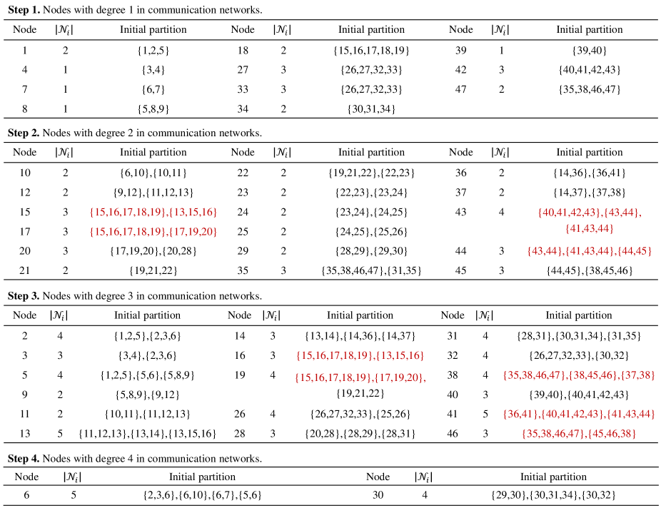
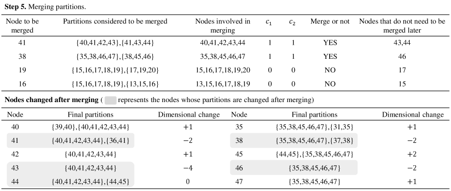
The following text explains Algorithm 1 and 2 in more detail with an example. Figure 4 shows the physical and communication network considered in this example, and The detailed steps of partitioning this network are listed in Figure 4 and Figure 5, where the former shows the initial partitioning steps and the latter shows the merging steps. To facilitate readers’ understanding, some key steps will be interpreted.
(I1) We focus on the area containing nodes . This area is taken as an example to show why partition design should be carried out in the order of . In light of the sorting rule, node with and is the first node to be considered. Based on line to line , we know . Hence, , , . Subsequently, partitions , , , , can be selected for nodes , , , and in order. Then, note that ; thus is necessary included in . Besides, since has been contained in , node needs not to select partitions any more. This reflects the advantages of the proposed node sorting rule: the node with a larger degree in the communication network selects the partition in the later order, which neither affects its partition selection nor interferes with the partition selection of the previous node, but greatly reduces the computational load (most of the required partitions have been selected in advance). The same situation can also be seen at node . However, the unreasonable order of nodes will lead to a large number of partitions with high repetition (See in I2).
(I2) We focus on nodes , , and . Their selection partition order is . Node selects its partition as . Hence, only node remains in . It means should be added into . However, since , must include a partition . It leads to a new partition to be added to node , which has completed the partition selection before that. More unreasonably, two highly repetition partitions exist at the same time in and . The reason for this phenomenon is that after the node selects its partitions. The above analysis shows that we have the advantage of allowing the node with a smaller communication network degree and larger physical network degree to select partitions preferentially. Otherwise, highly similar partitions like and will appear in large numbers. In addition, the above analysis also shows that a more reasonable sorting rule should be: node will preferentially select the partition if when . However, this sort rule means that one has to sort the nodes again after a node selects its partition, which is adverse to the implementation of the algorithm. Therefore, we do not improve the algorithm from the perspective of the remaining physical network neighbor nodes but use the merging strategy to make up for this problem.
(I3) Figure 5 displays the steps of merging partitions. Note that the actual calculation is not complex, although the complexity of the partition merging part is . It is because after the partitions of some nodes are merged, many other nodes that initially needed to merge partitions no longer need to perform the merging steps. For example, in Figure 4, all nodes need to merge partitions. However, (defined by Algorithm 2) with respect to node and are both empty after merging its partitions, and thus they need not perform the merging steps anymore.
Remark 2
From this example, we can see that if we design partitioned distributed observers based on the partitioning results shown in Figure 4 and 5, we can significantly reduce the dimension of observers on each agent. However, we must emphasize an important fact: the degree of reduction in observer dimension on agents is closely related to the similarity between the communication network and the physical network. Due to the arbitrariness of communication and physical networks, some strange partitions may occur. For example, two nodes that are neighbors in a physical network may be far apart in a communication network, which can lead to the occurrence of huge partitions. In such cases, the reduction in the dimension of observers on each agent will not be as pronounced as in Figure 4 and 5. Therefore, we introduce the concept of “network similarity”—defined by —to improve the rigor when describing simulation results. In other words, when describing how much our partition algorithm reduces the dimension of observers on each agent, we must indicate the degree of network similarity because the lower the network similarity, the higher the possibility of large abnormal partitions, and the lower the possibility of significant reduction in observer dimension.
III-B Partitioned distributed observer
This subsection designs distributed observer for each partition based on the partition method in the previous subsection. Suppose that is a partition belonging to , and then the state observer on the th agent to itself takes the form of:
| (8) |
where is the estimation of generated by observers on agent in partition ; with being the number of occurrences of in ; stands for the state estimation of the th subsystem generated by the th agent. is the high-gain matrix with and being the high-gain parameter; and are, respectively, the observer gain and coupling gain; is the so-called weighted matrix and is a symmetric positive definite matrix that will be designed later; is the control input relying on .
The dynamics of can be expressed as
| (9) |
where is the estimation of generated by observers on agent in partition , and is the control input relying on .
Denote and , we have
| (10) | ||||
| (11) |
where ; and is the actual control law employed in the closed-loop system.
Remark 3
This section has achieved the first goal of this paper through designing the partition algorithm and partition distributed observer: the dimension of observers on agent () is much smaller than that of the interconnected system.
Remark 4
There are two differences between the design of the partitioned distributed observer and the traditional distributed observer [13, 15]. First, since the states of the th subsystem may be repeatedly estimated by agent in multiple partitions, we introduce the fusion estimation () in the coupling part of observers on each agent. Second, agent needs to use the physical network neighbor information of agent when estimating the states of subsystem (see in (9)). In traditional distributed observers, this information can be directly found in observers on the th agent. However, since the dimension of observers on the th agent in this paper is much smaller than that of the interconnected system, its states fail to cover the neighbor states of subsystem . Therefore, we need to eliminate the coupling relationships ( in (9)) that cannot be obtained by agent when designing . In other words, to reduce the dimension of observers on each agent, we have to artificially introduce model mismatch to compensate for the lack of information caused by observer dimension reduction. Moreover, the control input in observers on the agent also needs the state estimation . So, multiple estimates and model mismatch also occur in the control input ( and ) of the partitioned distributed observer (8) and (9). The content introduced here is the novelty of the partitioned distributed observer design in this section, and it is also one of the main difficulties to be solved later.
IV Distributed control law for large-scale linear systems
Section III has reduced the dimension of observers on each agent by partitioning the network. This section will analyze the performance of the partitioned distributed observer and the closed-loop system after the dimension reduction of the local observer. Subsection IV-A shows the design of distributed control law. The stability of the error dynamics (10) and (11) and the closed-loop system will be proved in subsection IV-B and IV-C, respectively. Subsection IV-D will show the achievement of the second goal of this paper.
IV-A Distributed control law
State feedback control law can be employed in the large-scale system (3) and (4). By observing the dynamics of the th subsystem (1) and (2), the globally asymptotically stable control law gives rise to
| (12) |
where is designed so that is a Hurwitz matrix with . However, (12) is the state feedback control law with precise system states. Hence, one should replace them with the state estimations generated by the observers on the th agent. In the case of the traditional distributed-observer-based distributed control law [2, 9, 10, 11], the exact states of (12) can be directly replaced by state estimations of the th local observer. However, since this paper studies large-scale systems and does not want every agent to reconstruct all the states of the whole system, the concept of partition is introduced and thus leads to a fusion estimation problem (See Remark 4. For example, agent in the example of Figure 4 and Figure 5 has estimated its states three times in three partitions). Hence, , and (note that ) are expected to be employed in the control law of the th subsystem, i.e.,
| (13) |
Control law (13) can be used in observers on the th agent but not in closed-loop systems because it cannot protect the closed-loop performance from the peak phenomenon of observers. Hence, we need to add a saturation mechanism, i.e.,
| (14) |
where is the so-called saturation value of and it is expressed as with being a given positive constant and being the saturation function. Furthermore, in (9)—the control law with the state estimations of the th agent to the th subsystem—takes the form of:
| (15) |
Control law (12) is with precise and global states and is thus regarded as the centralized control law. (13) and (15) are employed in distributed observer (8) and (9). As for (14), it is the distributed-observer-based distributed control. The closed-loop system combined with (3) and (14) is the main research object of this paper.
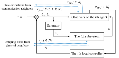
For the convenience of understanding, the diagram of the distributed control law described in this subsection is shown in Figure 6. As illustrated, the observers on the th agent use and the information obtained via the communication network to obtain required for the th agent. Then, observers send these to the th local controller to get and . Then, these control signals are used in observers of th agent, and —control signal after applying saturation mechanism—is used to control the th subsystem.
Lemma 2
There exists constants , , and such that
| (16) |
for and all , where .
Proof:
Since there is no finite time escape problem for linear systems, a constant exists such that the states of closed-loop system (3) and (14) are bounded when . Then, we know there are constants and such that and when . It follows . To continue, we first calculate
Consequently,
| (17) |
where . Denote , and . Then, we obtain
This completes the proof. ∎
Lemma 3
There are constants , , such that
| (18) |
for and all and , where .
Proof:
Similar to the proof of Lemma 2, there are and such that are bounded by when . Accordingly, we directly calculate
| (19) |
Then, defining , and yield the conclusion. ∎
This section has designed a distributed-observer-based distributed control law and analyzed the influence of model mismatch and fusion estimation in distributed observer on the control input. Since the local observer no longer reconstructs all the states of the interconnected system, there is a mismatch between and , as well as and . Therefore, the error forms and in this paper are difficult to express explicitly, which is different from the situation of the traditional distributed observer. Lemma 2 and Lemma 3 in this subsection effectively solve this problem by introducing finite time constraints. It is worth emphasizing that the finite time condition only plays an auxiliary role in this paper, and it will be abandoned in subsection IV-C.
In addition, a discussion about should be given. Designing the controller gain in this section requires the use of global information. This approach is to ensure a meaningful comparison between the performance of the distributed control law proposed in this paper and that of the centralized control law (at least, the form of the control law should be the same). In many practical systems, it is sufficient to achieve the performance of centralized control by designing the control gain in a distributed manner. For example, in problems such as unmanned vehicle formations and coordinated control of microgrids (including the majority of practical systems that high-order systems can represent), each agent can design its own control gain. Then, based on the information provided by the partitioned distributed observer, it is possible to achieve distributed control laws with centralized control performance.
IV-B Performance of partitioned distributed observer
This subsection mainly focuses on the stability of error dynamics of partitioned distributed observers. Before that, we need to provide an important lemma. Denote and then we can state the follows.
Lemma 4
Consider defined in Lemma 2 and . We have , and , where .
Proof:
We know and based on the definition of and . Hence,
Furthermore, by the inequality of arithmetic and geometric means, we have
Therefore, . ∎
Now, the main theorem of this subsection can be given. Note that this is a preliminary conclusion on the stability of error dynamics of partitioned distributed observers. The complete conclusion will be presented in Theorem 3 in the next subsection.
Theorem 1
Consider system (1), distributed observer (8)–(9), and networks subject to Assumption 1 and 2, and also consider the constant used in Lemma 2 and 3. Assume that states of closed-loop system (3) and (14) are bounded when . Then, for arbitrary , there is a such that the error dynamics of (8)–(9) can converge to an any small invariant set (around the origin) during if
1) is chosen as such that is a Hurwitz matrix (see more detail of in Remark 6) for all where and ;
2) is a symmetric positive definite matrix solved by
| (20) |
3) For all , coupling gain satisfies
| (21) |
where with , being the Laplacian matrix of the subgraph among as well as ; , , with , and with .
Proof:
Set and , then, based on equation (10), the dynamics of gives rise to
where . Denote and , then
where
To move on, we have
| (22) |
where , and is defined in Lemma 3. Besides,
| (23) |
where . Subsequently, the Lyapunov candidate can be chosen as , where
Then, based on (IV-B) and (IV-B), the derivative of along with gives rise to
| (24) |
According to conditions 1), 2), and Lemma 1, we have
| (25) |
where . Then, substituting (IV-B) into (IV-B) yields
Note that is equivalent to repeatedly calculating for all up to times and so does , where with . It leads thereby to
where . It is noticed that Lemma 4 leads to
and
where . Then, by denoting , and , we can further obtain
| (26) |
Condition 3) indicates that , and is obviously monotonically increasing and radially unbounded with respect to .
Equation (26) infers that is an invariant set. So, when is out of . Then, we obtain by the conclusion of [40] that
| (27) |
for all and some positive constants . It means
| (28) |
which shows that can converge to an any small invariant set in any short time by designing proper . In other words, one can choose a proper so that converges to for any . ∎
This section has proved that error dynamics of the partitioned distributed observer can converge to an any small invariant set before the given time . Due to the inability to analyze the performance of distributed observers and closed-loop systems separately, Theorem 1 relies on assumptions about . In Theorem 3 of the next subsection, we will provide a joint analysis of the observer and controller, where the assumption about will be removed. Next, we will further elaborate on some details and supplementary explanations of Theorem 1 in several remarks.
Remark 5
The design methods for the parameters of the partitioned distributed observer are detailed in Theorem 1. According to Theorem 1, all parameters except for only rely on the information of each individual agent and do not require any other information. Designing involves the information of system matrix, input matrix, and network topology. However, is actually just a sufficiently large constant. Therefore, in practical usage, it is often avoided to use global information by designing as an adaptive parameter.
Remark 6
Remark 7
Fusion estimation and model mismatch in partitioned distributed observer design make the stability analysis of its error dynamics (10)–(11) a real challenge because they not only bring more complex error dynamics but also derive two distinct compact error forms ( and ). In this subsection, Lemma 4 demonstrates the strict mathematical relationship between these two compact error forms. Then, Theorem 1 develops the two-layer Lyapunov analysis method, which ingeniously transforms the above mathematical relationship into the results that can be used in the traditional Lyapunov stability analysis. The proof of Lemma 4 and the design of the two-layer Lyapunov function () are the keys to successfully proving the error dynamic stability of the partitioned distributed observer.
IV-C Closed-loop performance under the distributed control law
This subsection first proves the performance of the closed-loop system under the assumption of stable observer error (Theorem 2). Then, we presents the joint analysis results of the observer and controller in Theorem 3, in which the stability analysis of the error dynamics of the distributed observer and the closed-loop system dynamics is completed (without relying on additional assumptions).
At the beginning, one obtains by centralized control law (12) that the closed-loop system with (12) is
| (29) |
Furthermore, the closed-loop system under distributed control law (13) takes the form of
| (30) |
Let , then the compact form of (IV-C) is expressed as
| (31) |
Now, we states the follows to show the performance of (31).
Theorem 2
Consider the closed-loop system (31) as well as its communication network and physical network subject to Assumption 1 and 2. If the error of the partitioned distributed observer (8)–(9) stays in with , then can converge to an invariant
where —given in the proof of Theorem 1—is a monotonically increasing function with respect to and radially unbounded. Furthermore, can be arbitrarily small with observer parameter tending to infinity.
Proof:
Since is Hurwitz, there is a symmetric positive definite matrix so that , where is a given constant. Then, the Lyapunov candidate can be chosen as . Its derivative along with (31) gives rise to
| (32) |
Based on (IV-A), we know . Hence,
| (33) |
It means that is an invariant set. Furthermore, since is a monotonically increasing function with respect to and radially unbounded, we have
| (34) |
Therefore, is an arbitrary small invariant. ∎
In what follows, we will focus on the closed-loop system with the distributed control (15) containing saturation mechanism:
| (35) |
This is the actual control law adopted by the closed-loop system in this paper, and also the source of output information in the partitioned distributed observer (8)–(9). Let and obtain the compact form
| (36) |
The following theorem will show the stability of (36).
Theorem 3
The distributed-observer-based distributed control law for large-scale system is given by (8)–(9) and (13)–(15). If we choose proper gains in (13) and observer parameters by Theorem 1, then the states of the closed-loop system (36) can converge to an invariant set
| (37) |
This set can be arbitrarily small when observer parameter tending to infinity.
Proof:
As a linear system, there is no finite time escape problem in the system (36). Hence, there are constants and so that for all . Then, in light of Theorem 1, we know there is a proper such that converges to during where is a constant satisfying .
Theorem 3 is of primary importance for this paper. It combines the conclusions of Theorem 1 and Theorem 2, and obtains the final result: the error system and the closed-loop system of the partitioned distributed observer can converge to any small invariant sets. Furthermore, the finite time conditions involved in Theorem 1 are eliminated by the analysis in Theorem 3. In fact, the final conclusion of the theorem only depends on the controllability and observability of the system as well as the connectivity of the communication network and does not depend on any other assumptions. These conclusions also indicate that, compared with the traditional distributed observer, the performance of the partitioned distributed observer in this paper has almost no loss, but the dimension of observers on each agent is greatly reduced. These results make the distributed observer more practical in large-scale system problems.
Remark 8
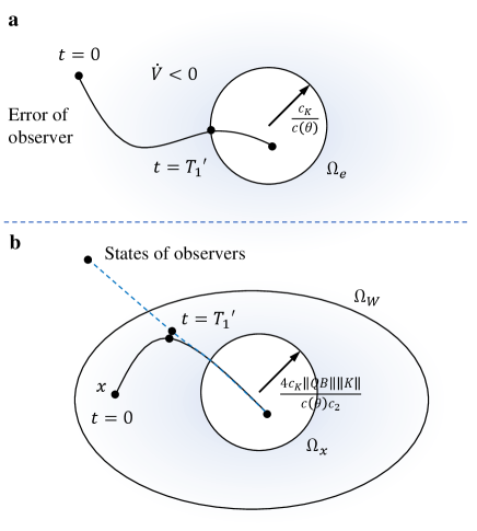
The proof of the stability of observer error dynamics and closed-loop systems mainly involves three steps. First, we assume that the states of the closed-loop system are bounded, and then the error dynamic can be proved to converge to when (see in Figure 7a). Second, we show that the states of the closed-loop system can converge to when is always in . Finally, as seen in Figure 7b, we assume that is the bound of the closed-loop system before . By designing , the trajectory of the observer can converge to the neighbor of the true states before escapes . After that, the distributed control law can control the dynamics of the closed-loop system to an arbitrarily small invariant set .
IV-D The ability of performance recovery
This subsection will show that the state trajectories of the closed-loop system (36) controlled by the distributed-observer-based distributed control law can approximate the trajectories of (29) arbitrarily. To this end, we denote the solution of closed-loop system (29) with initial states . Moreover, the solution of (36) is defined as with initial value . Note that the trajectories of depends on .
Theorem 4
The performance of distributed-observer-based distributed control law can approach that of the centralized control law arbitrarily, i.e., for any , there exists a constant and , such that for all .
Proof:
Since is chosen so that is a Hurwitz matrix, the system (29) is stable. Hence, there exists such that for all . Besides, according to Theorem 3, there is so that for all . Then, there is a constant such that for all and . Subsequently, we have
| (38) |
for arbitrary . Up to now, we have proved that holds on . In what follows, we will show it also holds on .
For this purpose, we construct a function , which satisfies and for , where is a function with .
We first consider the interval . Note that both and are bounded, as well as and are finite, thus there are two positive proportional functions and satisfying and when , which leads thereby to
for all , where . As a result, there exists a constant so that for arbitrary . Therefore, we have and .
Finally, we consider the scenario where . We define and , where is an implicit function of in light of Theorem 2 and 3. Since is a finite time interval, the conditions of the famous theorem (See in any monograph of “Ordinary Differential Equation”) named “The Continuous Dependence Theorem of Solutions of Differential Equations on Initial Values and Parameters” are fulfilled. It indicates that there is a constant such that if the parameter in satisfying . Bearing in mind the conclusion of Theorem 1 and 3, there exists such that for all .
Therefore, there exists so that , and . ∎
Up to now, the goals of this paper have been fully realized. After partition, the dimension of each local observer is far less than that of the interconnected system, but the distributed control law designed based on the partition distributed observer can still ensure that the controlled system can approximate the centralized control performance arbitrarily.
Remark 9
In the process of implementing the partitioned distributed observer and the distributed-observer-based distributed control law, the high-gain parameter plays an important role. However, it should be noted that the existence of high gain makes this method unable to deal directly with measurement noise. When measurement noise exists, there is a trade-off between the steady-state error (caused by measurement noise), the steady-state error (caused by model mismatch), and the difference between the distributed control performance and the centralized control performance. The smaller the latter two, the larger the former. Therefore, when both measurement noise and model mismatch exist, finding an optimal to consider these three indicators simultaneously is a topic that is worth further research in the future.
V Simulation
To illustrate the effectiveness of the developed methods, this section will be divided into three parts. Firstly, we describe the simulation system. Then, the effectiveness of the network partitioning method will be demonstrated. Finally, we show the validity of the partitioned distributed observer and the distributed-observer-based distributed control law.
V-A System formulation
The frequency subsystem of the droop control system contained in the microgrid system is considered. Assume that the large-scale system contains microgrids. Let be the electrical angle of the th generator, and be its angular velocity. Then, the dynamics of are governed by
| (39) | ||||
| (40) | ||||
| (41) |
where and represent the filter coefficient for measuring active power and frequency drop gain, respectively; stands for the expected active power; and is the voltage of the th microgrid system; represents the coupling relationship among microgrid and . Then, by linearizing the system (39)–(41) around the equilibrium point and denoting with and , we have
| (42) | ||||
| (43) |
where
The physical network and communication network corresponding to the system are both shown in Figure 2. and are the elements of their adjacency matrices, respectively. Therefore, the large-scale system considered in this section contains subsystems, i.e., .
In this paper, we randomly select within , and randomly select within . Besides, we choose for all .
V-B Effectiveness of partition method
It is seen from Figure 2 that the physical network and communication network among agents are different. We know by calculating the similarity between these two networks.
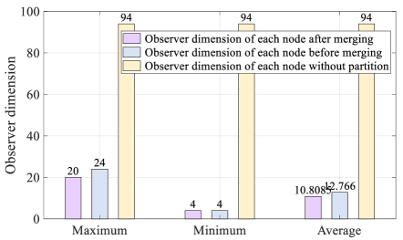
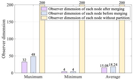
Each agent needs to estimate the whole system’s states if the classical distributed observer method [12, 13, 15, 16] is used. Therefore, the dimension of observers on each agent is . In contrast, it can be greatly reduced if the partitioned distributed observer developed in this paper is employed. See in Figure 8; the purple bar shows that, after partitioning, the maximum observer dimension of all agents is only (reduced by ), which is much lower than that of the traditional method (yellow bar). In addition, after partitioning, the minimum observer dimension on each agent is only (reduced by ), and the average value is only (reduced by ). Both of them are much lower than the value of the yellow bar. By the way, the merging partition process in Algorithm 1 in this paper can also effectively reduce the dimension of observers on each agent. By comparing the blue with purple bars, we see that the maximum and average values of the local observer dimensions after the partition merging (purple bar) are smaller than those before the partition merging (blue bar). Besides, through MATLAB simulation, the partition process of this example takes seconds.
To further illustrate the effectiveness of the partition algorithm, this paper also selects a system with nodes. Its physical network and communication network are shown in Figure 9. In this example, the similarity between the two networks is . As seen in Figure 10, compared to the traditional distributed observer, the maximum dimension of observers on each agent in the proposed partitioned distributed observer is reduced by , and the average dimension is reduced by . In this example, the time consumption of the partition algorithm by MATLAB is seconds.
In conclusion, the partition algorithm proposed in this paper can reduce the average local observer dimension by about when the similarity between the physical network and the communication network is about . Furthermore, the time consumption of the developed algorithm is very small.
V-C Performance of the distributed-observer-based distributed control law
We design the centralized control law of system (42) as
| (44) |
where and is chosen so that is a Hurwitz matrix. Subsequently, we obtain the distributed control law by designing a partitioned distributed observer.
The observer gains , and the weighted matrix can be calculated by Theorem 1 (Since there are different and , we will not show their specific forms). We set and randomly select the initial values of the closed-loop system within . In addition, the initial values of the partitioned distributed observer are all chosen as for all and all .
Then, the trajectories of the closed-loop system with different are shown in Figure 11. Subfigure a) is the trajectories of yielded by the centralized control law. Subfigures b), c), and d) are trajectories of , which is obtained by the distributed-observer-based distributed control law. From Figure 11d) and 11c), we know cannot converge to zero when high-gain parameter , while tends to zero when . However, it can be seen in Figure 11c) that the dynamic performance of with is still not as good as that of . When , we find that the trajectories in Figure 11b) are almost the same as that in Figure 11a). It indicates that the distributed-observer-based distributed control can achieve the same performance as that of the centralized control law.
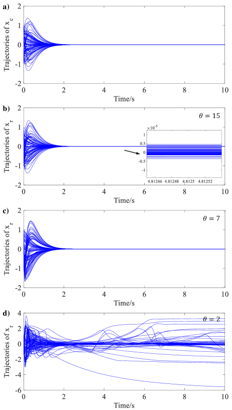
In addition, we need to point out that Figure 11 also shows the validity of Theorem 3. In this figure, closed-loop system states converge to a very small invariant set (The steady-state error shown in Figure 11b) is almost ). In addition, the premise that the closed-loop system states can converge to any small invariant set is that the state estimation error of the partitioned distributed observer can converge to any invariant set at any fast speed. Therefore, the excellent performance of the closed-loop system in Figure 11b) infers the excellent performance of the partitioned distributed observer.
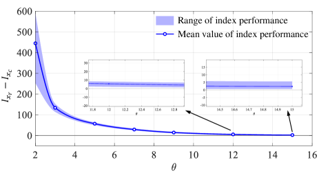
To further illustrate the ability of performance recovery, we selected , , , , , , and to show the approximation process of distributed-observer-based distributed control performance to centralized control performance. Define the performance index of the dynamic process as
| (45) |
Let and be the performance index of centralized control law and distributed control law, respectively. Then, Figure 12 shows how changes with . Since the initial values are randomly selected, we have simulated times for each to eliminate the influence of the randomness of the initial values. See in Figure 12, the blue dot represents the average value of corresponding to each , and the blue shadow represents the floating range of obtained from simulations. Simulation results show that the control performance of the distributed-observer-based distributed control law is infinitely close to that of the centralized control law.
It is worth mentioning that literature [2] also studied the distributed-observer-based distributed control law, which can arbitrarily approximate the centralized control performance. However, it studied small-scale systems, while this paper studies large-scale systems. Furthermore, according to the developed method in [2], the dimension of the local observer on each agent is equal to the dimension of the whole interconnected system. As a contrast, in this paper, the average dimension of observers on each agent is only of the interconnected system dimensions (See in Figure 8).
VI Conclusions
This paper has developed a distributed control law based on the partitioned distributed observer for large-scale interconnected linear systems. Firstly, we have designed a partitioning algorithm, which is achieved by two steps, including initializing and merging. The algorithm can significantly reduce the dimension of local observers. Secondly, the partitioned distributed observer for large-scale systems has been designed. To analyze the stability of its error dynamics, this paper has proposed the two-layer Lyapunov analysis method and proved the dynamic transformation lemma of compact errors. Finally, we have designed the distributed control law based on the developed partitioned distributed observer, which has been proved to have the ability to approximate the control performance of the centralized control arbitrarily. The simulation results have shown that the relative error between the performance of the distributed control law and that of the centralized control law is less than . Besides, the local observer dimension can be reduced by when the similarity between the communication network and the communication network is about .
References
- [1] X. Zhang, K. Movric, M. Sebek, W. Desmet, and C. Faria, “Distributed observer and controller design for spatially interconnected systems,” IEEE Transactions on Control Systems Technology, vol. 27, no. 1, pp. 1–13, 2019.
- [2] H. Xu, S. Liu, B. Wang, and J. Wang, “Distributed-observer-based distributed control law for affine nonlinear systems and its application on interconnected cruise control of intelligent vehicles,” IEEE Transactions on Intelligent Vehicles, vol. 8, no. 2, pp. 1874–1888, 2023.
- [3] H. Fawzi, P. Tabuada, and S. Diggavi, “Secure estimation and control for cyber-physical systems under adversarial attacks,” IEEE Transactions on Automatic Control, vol. 59, no. 6, pp. 1454–1467, 2014.
- [4] Y. Jiang, Y. Yang, S.-C. Tan, and S. Y. Hui, “Distributed sliding mode observer-based secondary control for DC microgrids under cyber-attacks,” IEEE Journal on Emerging and Selected Topics in Circuits and Systems, vol. 11, no. 1, pp. 144–154, 2021.
- [5] Y. Li, L. Liu, W. Yu, Y. Wang, and X. Guan, “Noncooperative mobile target tracking using multiple AUVs in anchor-free environments,” IEEE Internet of Things Journal, vol. 7, no. 10, pp. 9819–9833, 2020.
- [6] Y. Li, B. Li, W. Yu, S. Zhu, and X. Guan, “Cooperative localization based multi-AUV trajectory planning for target approaching in anchor-free environments,” IEEE Transactions on Vehicular Technology, vol. 71, no. 3, pp. 3092–3107, 2022.
- [7] K. Liu, J. Lv, and Z. Lin, “Design of distributed observers in the presence of arbitrarily large communication delays,” IEEE Transactions on Neural Networks and Learning Systems, vol. 29, no. 9, pp. 4447–4461, 2018.
- [8] H. Xu, S. Liu, S. Zhao, and J. Wang, “Distributed control for a class of nonlinear systems based on distributed high-gain observer,” ISA Transactions, vol. 138, pp. 329–340, 2023.
- [9] H. Xu and J. Wang, “Distributed observer-based control law with better dynamic performance based on distributed high-gain observer,” International Journal of Systems Science, vol. 51, no. 4, pp. 631–642, 2020.
- [10] B. Huang, Y. Zou, and Z. Meng, “Distributed-observer-based Nash equilibrium seeking algorithm for quadratic games with nonlinear dynamics,” IEEE Transactions on Systems, Man, and Cybernetics: Systems, vol. 51, no. 11, pp. 7260–7268, 2021.
- [11] T. Meng, Z. Lin, and Y. A. Shamash, “Distributed cooperative control of battery energy storage systems in DC microgrids,” IEEE/CAA Journal of Automatica Sinica, vol. 8, no. 3, pp. 606–616, 2021.
- [12] S. Battilotti and M. Mekhail, “Distributed estimation for nonlinear systems,” Automatica, vol. 107, pp. 562–573, 2019.
- [13] T. Kim, C. Lee, and H. Shim, “Completely decentralized design of distributed observer for linear systems,” IEEE Transactions on Automatic Control, vol. 65, no. 11, pp. 4664–4678, 2020.
- [14] M. Deghat, V. Ugrinovskii, I. Shames, and C. Langbort, “Detection and mitigation of biasing attacks on distributed estimation networks,” Automatica, vol. 99, pp. 369–381, 2019.
- [15] W. Han, H. L. Trentelman, Z. Wang, and Y. Shen, “A simple approach to distributed observer design for linear systems,” IEEE Transactions on Automatic Control, vol. 64, no. 1, pp. 329–336, 2019.
- [16] H. Xu, J. Wang, H. Wang, and B. Wang, “Distributed observers design for a class of nonlinear systems to achieve omniscience asymptotically via differential geometry,” International Journal of Robust and Nonlinear Control, vol. 31, no. 13, pp. 6288–6313, 2021.
- [17] C. Deng, C. Wen, J. Huang, X. Zhang, and Y. Zou, “Distributed observer-based cooperative control approach for uncertain nonlinear mass under event-triggered communication,” IEEE Transactions on Automatic Control, vol. 67, no. 5, pp. 2669–2676, 2022.
- [18] L. Wang and A. S. Morse, “A distributed observer for a time-invariant linear system,” IEEE Transactions on Automatic Control, vol. 63, no. 7, pp. 2123–2130, 2018.
- [19] K. Liu, Y. Chen, Z. Duan, and J. Lü, “Cooperative output regulation of LTI plant via distributed observers with local measurement,” IEEE Transactions on Cybernetics, vol. 48, no. 7, pp. 2181–2190, 2018.
- [20] G. Yang, H. Rezaee, A. Alessandri, and T. Parisini, “State estimation using a network of distributed observers with switching communication topology,” Automatica, vol. 147, p. 110690, 2023.
- [21] G. Yang, H. Rezaee, A. Serrani, and T. Parisini, “Sensor fault-tolerant state estimation by networks of distributed observers,” IEEE Transactions on Automatic Control, vol. 67, no. 10, pp. 5348–5360, 2022.
- [22] H. Xu, J. Wang, B. Wang, and I. Brahmia, “Distributed observer design for linear systems to achieve omniscience asymptotically under jointly connected switching networks,” IEEE Transactions on Cybernetics, vol. 52, no. 12, pp. 13 383–13 394, 2022.
- [23] H. Xu, S. Liu, B. Wang, and J. Wang, “Distributed observer design over directed switching topologies,” IEEE Transactions on Automatic Control, vol. pp, no. 99, pp. 1–14, 2024.
- [24] L. Wang, J. Liu, B. D. Anderson, and A. S. Morse, “Split-spectrum based distributed state estimation for linear systems,” Automatica, vol. 161, p. 111421, 2024.
- [25] E. Baum, Z. Liu, and O. Stursberg, “Distributed state estimation of linear systems with randomly switching communication graphs,” IEEE Control Systems Letters, vol. pp, no. 99, pp. 1–1, 2024.
- [26] P. Duan, Y. Lv, G. Wen, and M. Ogorzałek, “A framework on fully distributed state estimation and cooperative stabilization of LTI plants,” IEEE Transactions on Automatic Control, vol. pp, no. 99, pp. 1–1, 2024.
- [27] H. Su, Y. Wu, and W. Zheng, “Distributed observer for LTI systems under stochastic impulsive sequential attacks,” Automatica, vol. 159, p. 111370, 2024.
- [28] W. Han, H. L. Trentelman, Z. Wang, and Y. Shen, “Towards a minimal order distributed observer for linear systems,” Systems & Control Letters, vol. 114, pp. 59–65, 2018.
- [29] X. Wang, Z. Fan, Y. Zhou, and Y. Wan, “Distributed observer design of discrete-time complex dynamical systems with long-range interactions,” Journal of the Franklin Institute, vol. pp, no. 99, pp. 1–15, 2022.
- [30] A. Zecevic and D. Siljak, “A new approach to control design with overlapping information structure constraints,” Automatica, vol. 41, no. 2, pp. 265–272, 2005.
- [31] Y. Ding, C. Wang, and L. Xiao, “An adaptive partitioning scheme for sleep scheduling and topology control in wireless sensor networks,” IEEE Transactions on Parallel and Distributed Systems, vol. 20, no. 9, pp. 1352–1365, 2009.
- [32] H. Meyerhenke, P. Sanders, and C. Schulz, “Parallel graph partitioning for complex networks,” IEEE Transactions on Parallel and Distributed Systems, vol. 28, no. 9, pp. 2625–2638, 2017.
- [33] Y. Yang, Y. Sun, Q. Wang, F. Liu, and L. Zhu, “Fast power grid partition for voltage control with balanced-depth-based community detection algorithm,” IEEE Transactions on Power Systems, vol. 37, no. 2, pp. 1612–1622, 2022.
- [34] A. Condon and R. M. Karp, “Algorithms for graph partitioning on the planted partition model,” Random Structures and Algorithms, vol. 18, no. 2, pp. 221–232, 2001.
- [35] L. Wang, B. Yang, Y. Chen, X. Zhang, and J. Orchard, “Improving neural-network classifiers using nearest neighbor partitioning,” IEEE Transactions on Neural Networks and Learning Systems, vol. 28, no. 10, pp. 2255–2267, 2017.
- [36] H. Ruan, H. Gao, Y. Liu, L. Wang, and J. Liu, “Distributed voltage control in active distribution network considering renewable energy: A novel network partitioning method,” IEEE Transactions on Power Systems, vol. 35, no. 6, pp. 4220–4231, 2020.
- [37] E. Bakolas, “Distributed partitioning algorithms for locational optimization of multiagent networks in SE(2),” IEEE Transactions on Automatic Control, vol. 63, no. 1, pp. 101–116, 2018.
- [38] C. Shah and R. Wies, “Adaptive day-ahead prediction of resilient power distribution network partitions,” in 2021 IEEE Green Technologies Conference (GreenTech), 2021, pp. 477–483.
- [39] Y. Hong, G. Chen, and L. Bushnell, “Distributed observers design for leader-following control of multi-agent networks,” Automatica, vol. 44, no. 3, pp. 846–850, 2008.
- [40] H. K. Khalil, “High-gain observers in feedback control: Application to permanent magnet synchronous motors,” IEEE Control Systems Magazine, vol. 37, no. 3, pp. 25–41, 2017.