High order-accurate solution of scattering integral equations
with unbounded solutions at corners
Abstract
Although high-order Maxwell integral equation solvers provide significant advantages in terms of speed and accuracy over corresponding low-order integral methods, their performance significantly degrades in presence of non-smooth geometries—owing to field enhancement and singularities that arise at sharp edges and corners which, if left untreated, give rise to significant accuracy losses. The problem is particularly challenging in cases in which the “density” (i.e., the solution of the integral equation) tends to infinity at corners and edges—a difficulty that can be bypassed for 2D configurations, but which is unavoidable in 3D Maxwell integral formulations, wherein the component tangential to an edge of the electrical-current integral density vector tends to infinity at the edge. In order to tackle the problem this paper restricts attention to the simplest context in which the unbounded-density difficulty arises, namely, integral formulations in 2D space whose integral density blows up at corners; the strategies proposed, however, generalize directly to the 3D context. The novel methodologies presented in this paper yield high-order convergence for such challenging equations and achieve highly accurate solutions (even near edges and corners) without requiring a priori analysis of the geometry or use of singular bases.
Keywords: Electromagnetic Scattering, Acoustic Scattering, Integral Equations, Domains With Corners, Unbounded Solutions at Corners, High-Order Accuracy
1 Introduction
The computational solution of electromagnetic scattering problems plays fundamental roles in many areas of science and engineering, ranging from photonics to remote sensing, and including communications, optics and electromagnetic compatibility among many others. Computational electromagnetic scattering solvers based on boundary-integral equation (BIE) offer a number of advantages, such as reliance on discretizations of lower dimensionality; an ability to directly utilize CAD geometries as input without significant geometry processing, and associated faithfulness to the geometries provided; a lack of dispersion errors of significance; and, when used in conjunction with suitable acceleration methods [6, 7, 13, 15], high efficiency in terms of computing times and parallel performance. The Chebyshev-based “rectangular-polar” Boundary Integral Equation (RP) method [12, 28] is a computationally efficient, high-order Nyström method for the discretization and solution of scattering and radiation problems in 2D and 3D which, based on use of representation of surface currents in terms of local Chebyshev polynomial expansions, achieves high-order accuracy for smooth geometries. The method’s convergence rate, however, can drop to even less than linear for practical geometries that include geometric singularities such as sharp edges and corners, thus eliminating, in such cases, one of the significant benefits offered by the methodology. The difficulty arises from the singular behavior of field components and current densities (and/or their derivatives) near geometric singularities. This behavior leads to poor numerical approximations and significant integration errors in these regions. The challenge is further exacerbated in cases where the solution of the integral equation (the “density”) diverges at corners and edges. While such issues can often be circumvented in 2D configurations , they are unavoidable in 3D Maxwell integral formulations, where the tangential component of the current-density vector along an edge becomes infinite. While such singular fields near an edge can be represented by an asymptotic expansion of quasistatic singular fields, which can in turn be incorporated in numerical methods in the form of singular basis functions, unfortunately, algorithms based on such approaches may suffer from significantly increased complexity in view of the geometrical dependence of the singular exponents involved—which, in particular, are not even known in closed form for corners in 3D space and would thus require numerical evaluation, which in itself amounts to a challenging computational problem.
In order to tackle the problem at hand, this paper restricts attention to the simplest context in which the unbounded-density difficulty arises, namely, an integral formulation in 2D space whose integral density blows up at corners. The novel methodologies presented in what follows recover high-order convergence for such challenging geometries, and they achieve highly accurate solutions (even near edges and corners) without requiring a priori analysis of the geometry or use of singular bases. In detail, this paper considers a prototypical integral-equation (for the 2D Neumann problem for the Helmhotz equation) whose density solution is unbounded at corners. Alternative integral equation formulations can be used for the 2D Neumann-Helmholtz problem considered here: for example, the surface currents associated with the Direct Regularized Combined Field Integral Equations (DCFIE-R) for the Neumann problem are bounded near edges and corners , and they are thus amenable to effective treatment by means of well known regularization methods. Our selection of integral equation with unbounded density was made, precisely, to enable the development of strategies capable to accurately deal with infinite densities, which could then be generalized and applied in the corresponding 3D cases for which, as mentioned above, infinite densities at edges and corners exist regardless of the formulation used. As discused below, the novel methodologies presented in this paper yield high-order convergence for such challenging geometries and achieve highly accurate solutions (even near edges and corners) without requiring a priori analysis of the geometry or use of singular bases.
The following discussion provides a brief review of the literature, beginning with contributions on finite element methods (FEM) for partial differential equations (PDEs) in domains with geometric singularities. While FEM results in sparse systems of linear equations, these methods are not always competitive with integral equation methods. The latter, leveraging lower-dimensional discretizations, can benefit from fast solvers [13, 7, 34] and, when applicable, significantly outperform FEM approaches. Nonetheless, FEM-based techniques for boundary value problems in domains with singular boundaries are crucial in many fields and have inspired a rich body of research. For instance, spatially refined meshes near regions of geometric singularities have been explored in [4, 17, 37, 5, 19, 20]. An alternative approach explicitly incorporates the known singular behavior into the Galerkin basis, as discussed in [35, 21, 32, 29]. The “DtN finite element method,” detailed in [23, 39, 38], identifies neighborhoods of corner singularities and poses a new boundary value problem on the complement of these neighborhoods using artificial boundary conditions derived from Dirichlet-to-Neumann maps.
Green function-based integral equation methods, in turn, particularly high-order techniques for solving two- and three-dimensional problems in domains with smooth boundaries, are well-established [30, 13, 22, 36]. Significant advancements have also been achieved for non-smooth domains, as demonstrated by works such as [33, 2]. For instance, the approach in [33] utilizes theoretically robust first-kind (singular or hypersingular) integral equations combined with high-order Galerkin boundary element methods. These techniques are effective for both Dirichlet and Neumann problems; however, they exhibit limited accuracy in scenarios where the integral equation solutions, as considered in this study, become unbounded [27].
Nyström-based integral-equation methodologies, which align more closely with the approach proposed here, have also been applied with notable success [31, 3, 24]; a comprehensive discussion of this literature can be found in [2, Chap. 8]. These methodologies use special graded-mesh quadratures to achieve high-order accuracy for solving the Dirichlet problem for the Laplace equation in two-dimensional domains with corners via second-kind integral equations. However, the integral equations addressed in these contributions do not involve hypersingular operators, which are central to the present study. As demonstrated in Section 4.1, directly extending these methods to Maxwell problems which involve hypersingular operators as well as unbounded integral densities does not generally yield accurate solutions. Additional Nyström methodologies including both hypersingular operators and unbounded solutions are presented in [9, 26] and references therein. Reference [9] builds upon the “augmented” integral equation method [40], in that it relies on use of integral operators supported in curves in the interior of the obstacle—which may pose some challenges for realistic 3D configurations. The method demonstrates high accuracies of the computed fields, albeit at significant distances from the corner points. Reference [26], in turn, presents the recursive “RCIP” method, which recursively subdivides regions near corners. That reference presents highly accurate results for a domain with a corner, and it indicates that the opening angle should be in the interval .
This paper presents a numerical methodology that recovers high-order convergence in presence of unbounded densities at corners, and which produces highly accurate solutions even at extremely close proximity from the singularity and for extremely sharp corners (such as, e.g., near machine precision accuracy at a distance for a corner with an interior angle of radians ); it is expected that forthcoming 3D versions of the proposed algorithm will prove similarly effective. The proposed approach utilizes (i) A regularized-operator integral formulation (Section 3.1) that eliminates the deleterious spectral character arising from hypersingular operators inherent in the integral formulation; and, (ii) A regularization procedure and associated regular density unknown that incorporates a corner-regularization Jacobian factor (Section 3.2); together with, (iii) Specialized near-corner and self-interaction quadrature techniques that effectively manage the extreme proximity of discretization points, and associated cancellation errors, that are introduced by the corner regularization methods (Sections 3.3 and 3.4). A variety of numerical examples provided in this paper illustrate the character of the proposed approach. Results for the wave-equation solution with near machine-precision accuracy are obtained arbitrarily close to the corner: such accuracies are indeed consistently demonstrated in this paper at a nominal extremely-close distance of away from corners (see Remark 1 for additional details in this regard).
This paper is organized as follows. Section 2 presents necessary background concerning integral equations (which give rise to infinite densities at corners), and it reviews the Chebyshev-based (Nyström) rectangular polar discretization method [12, 28]. Section 3 then presents the proposed strategy for high-order solution of the infinite-density problem, which involves use of a change of integration variables and associated graded meshes as well as a change of unknown, and which requires in particular detailed treatment of arithmetic near-limits of the form in finite-precision arithmetic. A variety of numerical results illustrating the character of the proposed methods are presented in Section 4, and a few concluding remarks, finally, are provided in Section 5.
2 Integral Equation Formulations for Smooth Surfaces
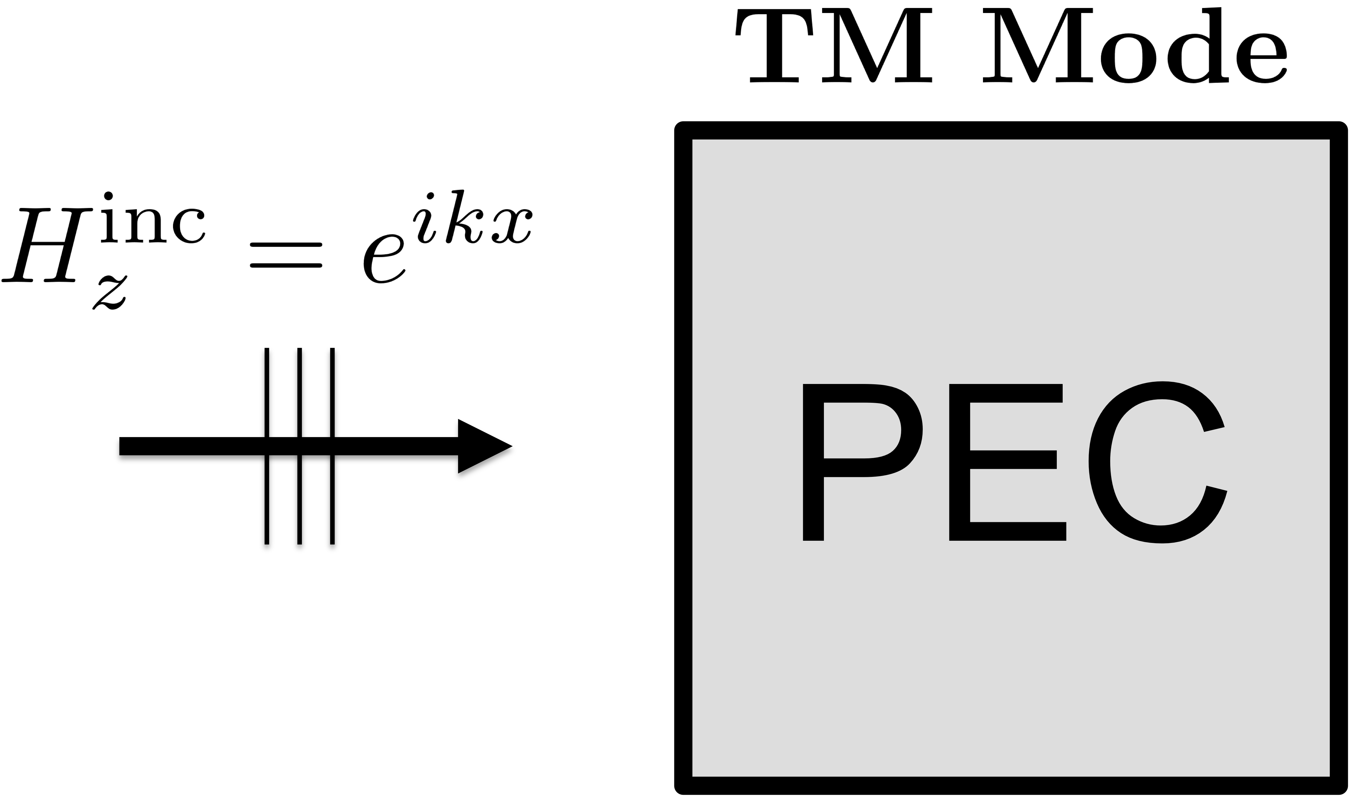
We consider the problem of scattering of Transverse Magnetic (TM) Electromagnetic waves by a closed perfect electrical conductor (PEC) scatterer with boundary in 2D space, wherein the spatial variable is used, under an incident wave with transverse magnetic-field component such as, e.g. . The resulting electromagnetic scattered field in the domain exterior to can be determined on the basis of the transverse scattered magnetic field component , which is a solution of the problem
| (1) | |||
| (2) |
2.1 Magnetic Field Integral Equation
Using the single-layer representation
| (3) |
where
| (4) |
denotes the outgoing Helmholtz free-space Green’s function, the imposition of the Neumann boundary condition (2) results in the Magnetic Field Integral Equation (MFIE) [16]
| (5) |
Once a solution of this equation has been produced and substituted into (3), the solution of (1)-(2) can be obtained by straightforward numerical quadrature.
The MFIE (5) is not uniquely solvable at a scatterer-dependent countable sequence of frequencies , see e.g. [16], around each one of which the associated numerical implementations become ill-conditioned and inaccurate. This problem can be eliminated by utilizing instead a certain combined field integral equation formulation, which is considered in Section 2.2. Unfortunately, however, that formulation incorporates a hypersingular operator whose practical implementation presents certain difficulties, most notably in terms of the associated conditioning characteristics and large iteration numbers it requires if iterative solvers are used for its solution. Following [11], Section 3.1 introduces a second version of the combined equation, where the hypersingular operator is regularized using a smoothing operator. This approach resolves the difficulties associated with the hypersingular nature of the problem, at least for smooth surfaces . However, new complications emerge when this formulation is applied to domains with corners, since, as is the case for the regular CFIE formulation, its solutions are unbounded at corner points. An additional reformulation of the problem, that introduces the new corner-regularized unknown and associated equation, which is one of the key contributions in this paper, is then presented in Section 3.2. Sections 3.3 and 3.4 detail additional components of the proposed solver designed to address finite precision issues associated with the use of fine singularity-resolving meshes and fine-scale pre-computation problems. The remainder of the present Section 2, in turn, introduces the aforementioned smooth-surface uniquely solvable CFIE equation and associated parametrization and differentiation methods, which are needed for reference in the subsequent Section 3.
2.2 Unique Solvability: Combined Field Integral Equation
Using now the representation
| (6) |
instead of (3) (see [11] and references therein), enforcement of the Neumann boundary conditions (2) yields the Combined Field Integral Equation (CFIE) formulation
| (7) |
where is a coupling parameter. Following [11], throughout this paper the value is used. In equation (7) and throughout this paper, (resp. ) denotes differentiation with respect to in the direction of (resp. differentiation with respect to in the direction of ). The last operator on the left-hand side of (7), namely, the normal derivative of the double-layer operator, is a hypersingular operator—whose computation by direct implementation of normal derivatives can be rather challenging. Fortunately, however, the hypersingular operator may be expressed in the form
| (8) |
(see [11] and references therein), where and denote the operators of differentiation with respect to the unit tangent vectors and at the respective “target” and “source” points and on ; clearly equation (8) does not require evaluation of derivatives in directions other than those tangential to , and can therefore be computed effectively by means of the discretization methods used in this paper. (Note that the identity (8) holds for closed curves, provided the tangential vector is defined in a consistent manner throughout the scatterer’s boundary, e.g., in counterclockwise fashion.) In sum, defining the operators
| (9) |
| (10) |
| (11) |
the CFIE equation (7) takes the form
| (12) |
Note that the integrals required by the operators and may be expressed in the forms
| (13) |
while may be presented in the form
| (14) |
for certain kernels and functions : we have and for the operator ; and for the operator ; and and for the opeator . Clearly, the operator requires an additional differentiation of the unknown —which, as discussed in. [11], impacts significantly upon the accuracy and conditioning of the resulting numerical implementation.
In preparation for the introduction of the main operator- and corner-regularization methods in Section 3, the following two sections describe, in the context of smooth surfaces, the particular parametrization and discretization methods used, and the associated methods employed for differentiation of surface variables and evaluation of Green function-based integral operators.
2.3 Chebyshev-Based Parametrization and Rectangular-Polar Integration: smooth-scatterer case
Throughout this paper the discretizations of integral operators such as those considered in the previous sections and elsewhere are implemented on the basis of of the Chebyshev-based Rectangular Polar (RP) Nyström methods introduced in [12, 28]. This section briefly reviews the RP method as it applies in the context of smooth surfaces and for operators that do not contain tangential differentiation (e.g., the operators (9) and (10) above); additions presented in Section 2.4 then enable the discretization of the operator (11) with similar efficiency and accuracy.
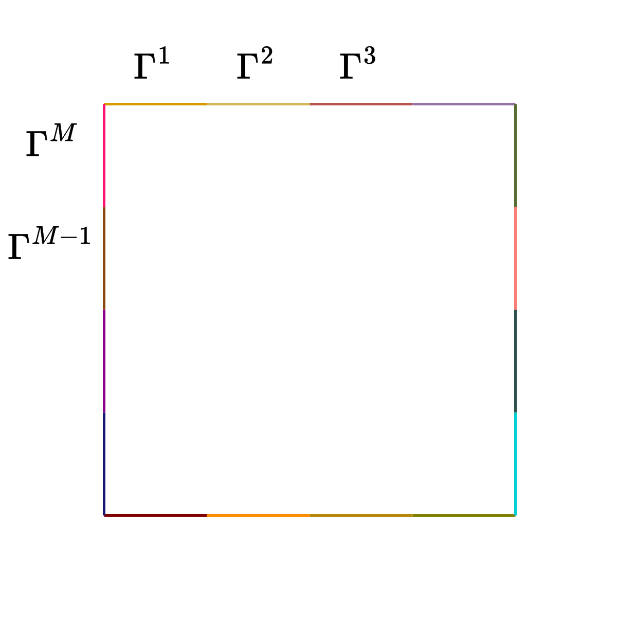
The RP method relies on use of a partition of curve (surface in 3D) into a set a set of non-overlapping patches
| (15) |
as depicted in Figure 1. Without loss of generality it is assumed that each curve is parametrized by a vector function with scalar argument
| (16) |
(Note that, while previous implementations of the RP method use patch parametrizations defined in the interval —given the reliance of the RP method on Chebyshev expansions—, throughout this paper the parameter segment is utilized instead, on account of the “zero-centering” technique introduced per Sections 3.2 and 3.3, which requires the use of such a parametrization interval.)
On the basis of the parametrizations , a function defined on corresponds to the function defined for , which can then be discretized by means of the -point Chebyshev grid given by [8]
| (17) |
where
| (18) |
Clearly, using points per patch for a total , the total number of discretization points used is
| (19) |
The implementation of the integral operators at hand requires consideration of the line element
| (20) |
as well as the unit tangential and normal basis vectors which, at a point , are given by
| (21) |
In order to achieve high computational efficiency and accuracy the RP quadrature algorithm proceeds by separately treating singular, near-singular, and regular interactions. In view of (13) and (15), the integral may be expressed in the form
| (22) |
where
| (23) |
For target points away from the source patch (as determined by a certain proximity parameter ) the kernels of the integral operators are smooth over the source patch, and, at least in the smooth-surface case considered in this section, so are the density functions ; thus, for such far interactions (on smooth domains) the method directly utilizes Fejér’s first quadrature rule for integration, and the approximation
| (24) |
results, where and denote the integration points and weights introduced in equation (17).
When the target point is close to or within the source patch, on the other hand, the kernels of the integral operators are near singular or singular, respectively, and accurate evaluation of the corresponding integrals requires use of specialized integration techniques. To produce such integrals, the RP method relies on the Chebyshev approximation
| (25) |
which can be obtained for the necessary functions (equal either to or its tangential derivative, see equation (14)) from the available values of the density on the Chebyshev mesh. Using this expansion, the operator values in singular and near-singular cases can be efficiently and accurately computed on the basis of the numerically precomputed integration weights
| (26) |
These weights can be precomputed by integrating the kernel against each Chebyshev polynomial (e.g., as described in [12, 28]) and stored for repeated use. Using these weights we obtain the accurate approximation
| (27) |
This approach applies to each one of the kernels listed near the end of Section 2.2 and, together with the aforementioned smooth integration methods for far from , it enables the necessary integrals over to be computed efficiently via equation (22). Note that, per the discussion above in this section, precomputations are necessary for target discretization points on the source patch , as well as for near singular target discretization points on the nearby patches for which the distance between the discretization points and is less than .
2.4 Differentiation
The evaluation of the operator in (11), which contains two tangential derivatives, is discussed in what follows. In view of (15) and writing
| (28) |
(since and ), it suffices to evaluate the right-hand side expression in this equation for all and with and then sum over for each . To do this we leverage the Chebyshev structure inherent in the RP algorithm described in Section 2.3 together with the numerically stable Chebyshev differentiation approach [8] (which is briefly reviewed below), all of which results in the following procedure.
-
1.
For each evaluate the derivative for using Chebyshev differentiation.
-
2.
For each and each evaluate the integral by means of the RP methods described in Section 2.3 with and on the basis of the quantity obtained per point 1, and then obtain the quantity .
-
3.
Calculate using once again Chebyshev differentiation.
The aforementioned Chebyshev-based differentiation algorithm [8] numerically obtains the derivative of a given function defined in the interval as follows:
-
(a)
Obtain the Chebyshev expansion of order (throughout this paper we have used the value for differentiation purposes);
-
(b)
Obtain the derivative coefficients by means of the recurrence relation
-
(c)
Evaluate the desired derivative values via the inverse Chebyshev transform .
3 Operator-Regularized and Corner-Regularized Combined Field Integral equations
3.1 Operator-Regularized Combined Field Integral Equation: A Well-Conditioned Smooth-Boundary Formulation
Computational experiments presented in [11] illustrate the fact that, while the CFIE formulation is uniquely solvable for all wavenumbers, solving it accurately can give rise to certain difficulties. The presence of two tangential derivatives in the hypersingular operator (8) associated with the formulation (7) induces arbitrarily large eigenvalues as the discretizations are refined. As a result, the conditioning of the system suffers and the numbers of iterations for convergence to a required tolerance increases significantly. As shown in [11] these difficulties can be effectively resolved, for smooth surfaces , by representing the scattered fields in the alternative form
| (29) |
where
| (30) |
is a regularizing operator. The wavenumber can take any real or imaginary values and does not necessarily need to depend on the wavenumeber of the problem , but [11] recommends the use of the value
Enforcement of the Neumann condition (2) then gives rise to the (Operator) Regularized Combined Field Integral Equation (CFIE-R)
| (31) |
As illustrated in [11], at least for smooth surfaces, this formulation leads to well conditioned numerical methods which additionally, if used in conjunction with iterative solvers, require reduced iteration numbers. But the equation suffers from severe accuracy and conditioning problems for surfaces containing corners. A “Corner-Regularized” discretization is introduced in Section 3.2; unlike the operator regularization introduced in the present section, the corner regularization is introduced on the basis of the parameterizations of the various smooth curves that make up the piecewise-smooth scatterer . Since the RP discretization method [12, 28] utilized in this paper otherwise relies on use of certain parametrizations and discretizations of in terms of cosine transforms and Chebyshev polynomials, for conciseness Section 3.2 introduces the corner-regularization method on the basis of such parametrizations. We should note, however, that, (i) The corner regularization method presented in Section 3.2 could also be implemented in connection with other Nyström or Boundary-Element discretizations; and, (ii) It is expected that, in conjunction with the electromagnetic operator-regularized equations presented in [10] (3D Maxwell analogous of the ones described in Section 2.2), the methods inherent in the corner-regularized version of of the RP method presented in Section 3.2 should provide an excellent basis for a 3D-Maxwell corner-and-edge regularization methodology.
3.2 Corner-Regularizing Change of Unknown: Regularization of Unbounded Densities
The proposed corner-regularization approach partitions the domain into a set of non-overlapping patches, parameterized by the functions , , each one of which contains either one corner or no corners, and it is assumed that, by construction, if the -th patch contains a corner then the corner point equals —that is, the corner point corresponds to the parameter value —a feature that is utilized to eliminate catastrophic cancellation errors in the context of Section 3.3. Note that, in view of this prescription, the tangential vectors obtained by direct differentiation of the parametrization on some of the patches need to be flipped (multiplied by ) in order to obtain a consistent prescription (say, counterclockwise) of the tangential vector field around .
The regularization method used seeks to yield an integral formulation whose unknown density is bounded and sufficiently smooth at corners. To do this, the algorithm relies on the use of a 1-1 change of variables (CoV) , for each patch containing a corner [16, 31, 25]. The corner CoV gives rise to an integration Jacobian that vanishes at the corner together with its derivatives up to a prescribed order, and it maps a uniform mesh in the variable to a mesh in the variable that is graded toward the corner. The CoV Jacobians, which appear in the integrand multiplying the unknown density, are such that the product of Jacobian and density has a number of bounded derivatives at the corner point—thus resulting in a “regularized” quantity which can be approximated closely by the Chebyshev expansions used in the RP method.
Regularizing CoVs have previously been used for regularization of bounded (Lipschitz continuous) integral densities [16, 31, 25]; the regularization strategy embodied in equations (41) and (44) below, which is applicable to integral equations whose density solutions are unbounded, is one of the main enabling elements introduced in this paper. Other essential algorithmic elements in the proposed approach are introduced in Sections 3.3 and 3.4.
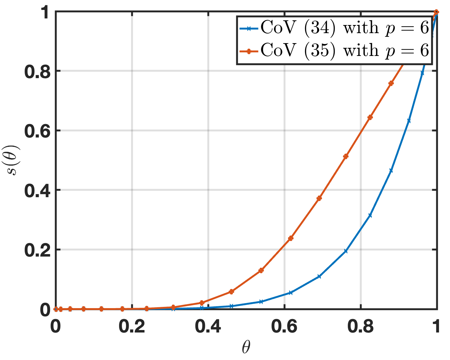
Per equation (35) below the changes of variables utilized in this paper are based on use of the CoV function [16, 31]
| (32) |
which is depicted in Figure 2, where
The derivatives of the function of orders less than or equal to vanish at and —so that, in particular, we have
| (33) |
While simpler changes of variables such as the monomial CoV [25]
| (34) |
of whose derivatives vanish at can also be effective, the CoV (32), which is used throughout this paper (with exception of the comparison results presented in Figure 12 right), gives rise to significantly better performance than the simpler version (34) on account of the rather evenly split distribution it enjoys of dicretization points near to and away from the endpoints of the interval [16]. Results based on the monomial change of variables (34) presented in Figure 12 right provide an indication of the improvements that result from the use of the CoV (32).
Recalling that, as indicated at the beginning of this section, corners are assumed to occur only at points, on any one of the patches the CoV is induced by the change of variables (32) in accordance with the expression
| (35) |
Note that the first derivatives of vanish at for patches containing a corner and for patches not containing a corner.
Incorporating the CoV (35) and defining
| (36) |
the adjoint double-layer integral in (31) (that is, the first integral on the left-hand side in that equation) with becomes
| (37) |
(It is important to recall that, in view of the definitions and assumptions introduced above in this section, for patches containing a corner , the corner point is necessarily given by .) The regularization operator (30), in turn, takes the form
| (38) |
Similarly, for the last two integrals in (31) we obtain the expressions
| (39) |
and
| (40) |
respectively.
In all, incorporating the CoV (35) in (31), using the expressions (37) through (40), and multiplying the result by , we obtain
| (41) |
Thus, defining the new unknown
| (42) |
and expressing the regularization operator (38) in the form
| (43) |
we finally obtain the change-of-unknown, Corner-Regularized version
| (44) |
of the Operator Regularized R-CFIE equation (31). It is important to emphasize that is a much smoother function than (and, thus, significantly easier to approximate by polynomials) on account of the multiplicative line element factor contained in , whose value together with that of of its derivatives, vanishes at the corner point where the field singularity is located. This is another key aspect of the proposed methodology for scattering by domains with corners.
For the purpose of comparison in the numerical results section we additionally consider the following change-of-unknown, corner-regularized version of the MFIE equation (5):
| (45) |
Note that in light of the introduction of the new unknown , which includes a the factor, the rectangular polar discretization method needs to be modified as follows:
-
1.
Substitute the Fejér evaluation of the far interactions (24) by the corresponding Fejér approximation
(46) - 2.
-
3.
Replace the precomputation integrals (26) by
(48) for the kernels listed near the end of Section 2.2, and for target discretization points on the source patch , as well as for near singular target discretization points on nearby patches . (Note that, in particular, the factor, which is contained in the new unknown , does not appear in the integrand of equation (48).) In view of the singularities introduced by the corner geometries under consideration, certain significant variations of the rectangular polar method [12, 28] are needed, which are described in Sections 3.3 and 3.4.
-
4.
Using the precomputed weights (48) evaluate the integral
(49) in terms of the coefficients in (47), and evaluate the needed overall integrals by a sum analogous to (22). The tangential differentiations needed for the evaluation of the operator in (14) are produced by a procedure analogous to the one described in Section 2.4 applied in the variable (instead of the variable used in that section).
3.3 Finite precision evaluation of Green-function source-target interactions
The introduction of the CoV and associated change of unknown, which effectively enables the approximation of the new integral densities in terms of corresponding Chebyshev expansions, can also give rise to significant numerical cancellation errors unless suitable numerical procedures are used, on account of the finite precision inherent in computer arithmetic. The strategies we use to eliminate cancellation errors for “near-corner interactions” and “self interactions” are described in what follows. Note that, in view of the overall strategy used, source-target near interactions only arise as part of the precomputation stage described in Section 3.4.
Let us consider a corner point located at the intersection of the patches and , , for which, in accordance with the conventions put forth in Section 3.2, we have . Clearly, the CoV introduced in that section generally induces graded meshes that can result in marked clustering of points near on both the source and target patches ( and respectively). The resulting extreme proximity of source and target points (generically) gives rise to catastrophic cancellation in the evaluation of certain source-target differences that are required for evaluation of Green-function values. In detail, catastrophic cancellations occur for source and target points and near if at least one of the coordinates of is an quantity. Indeed, if a source discretization point and a target discretization point are each within a distance from the corner, where , the resulting computation of the difference would suffer from a significant cancellation error: a loss of a number of digits would ensue from such a calculation. Taking into account the small values that may arise in this context (e.g., the numerical examples presented in this paper feature values in the range for and for with , ) the accuracy loss can be highly detrimental. Accurately computing these small quantities (and associated large Hankel-function values) is crucial to produce the necessary and correct contributions to the values of the solution both near and away from the corner point.
Large source-target cancellation errors arise across smooth portions of the surface as well, in view of the need for evaluating the normal derivative of the Green function in such regions. Cancellation errors also affect the Green function itself, which also appears in equations (10) and (11), but the cancellation-error difficulty is particularly problematic in the context of the adjoint double-layer operator (9) since the normal derivative contains the term
| (50) |
The issue stems from the quadratic decay of the numerator in (50), whose magnitude decreases like as , at points where the surface is smooth, and whose resulting (large) relative errors are then amplified upon division by the small denominator . Fortunately such errors can be effectively treated by using a Taylor expansion of the the parametrization around . Neighboring pairs of points and that are additionally near corners, whether they are on the same patch () or on different patches (), require a somewhat different treament, in view of the corner changes of variables and associated fine refinements utilized by the proposed algorithm—which may compound the degree of proximity, but which would be cumbersome to treat via Taylor expansions on account of the multiple-derivative vanishing at corners that is induced by the corner changes of variables parametrization. To tackle the near corner cancellation problem around a corner point we consider the parametrizations and of the two patches that contain the point (possibly with )—so that, in accordance with the prescriptions in Section 3.2 we have . In view of the first equation in (36) our algorithm incorporates the lowest order Taylor expansions (with remainder) and so that . Since in view (33) and (35) of the changes of variables satisfy and , this procedure produces as the difference of two suitably small numbers thereby bypassing the near-corner cancellation problem. (Note that in the case the algorithm additional incoporates the aforementioned Taylor expansion in around , thereby leading to accurate evaluation of small differences throughout .)
.
3.4 Numerical treatment of pre-computations
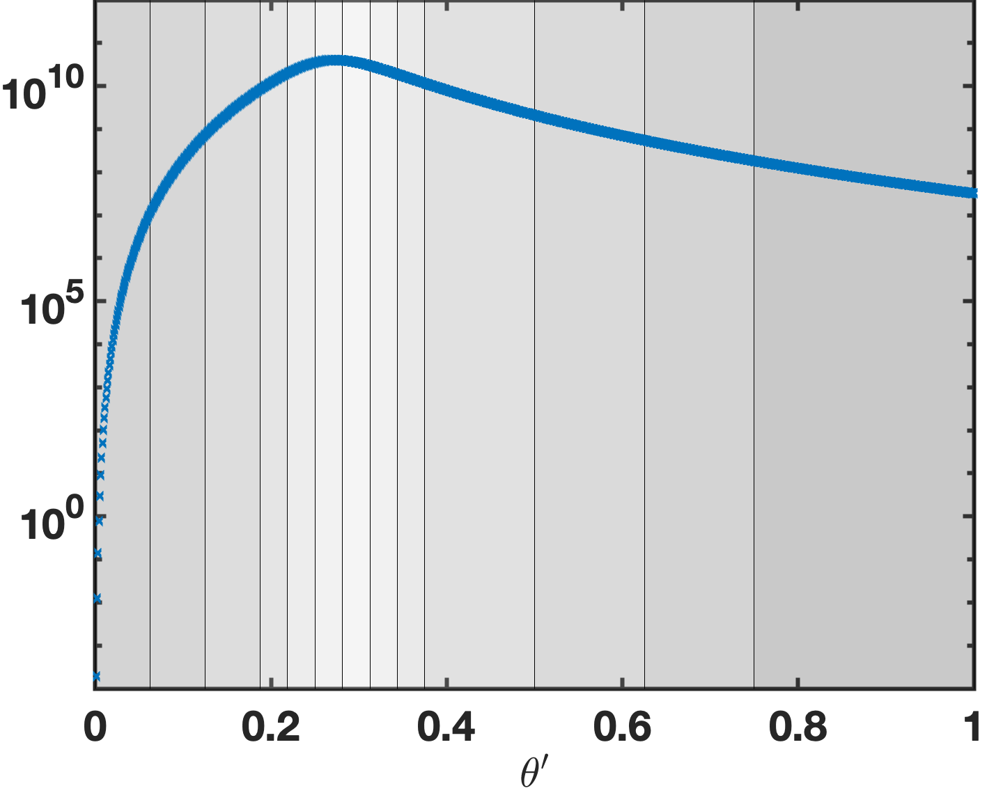
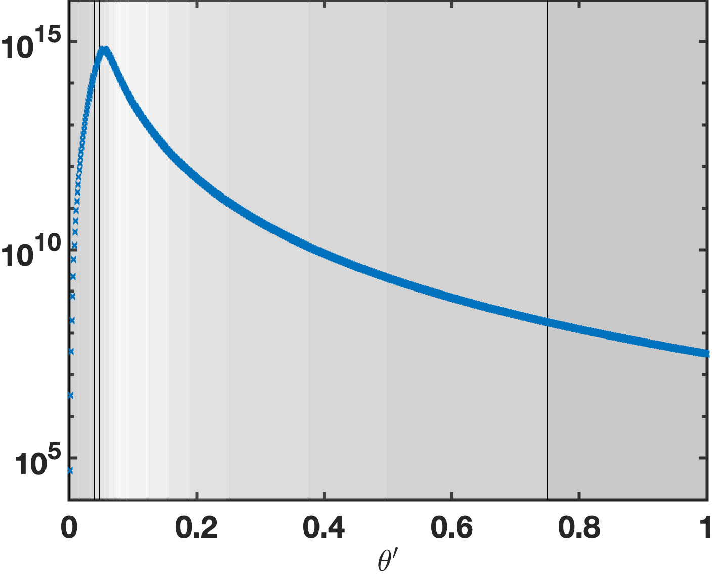
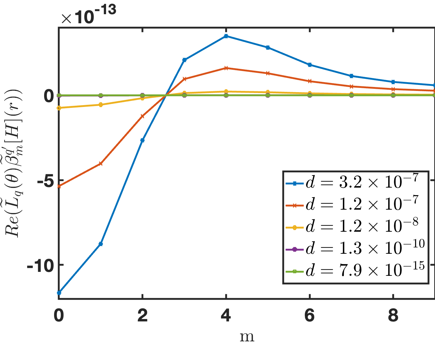
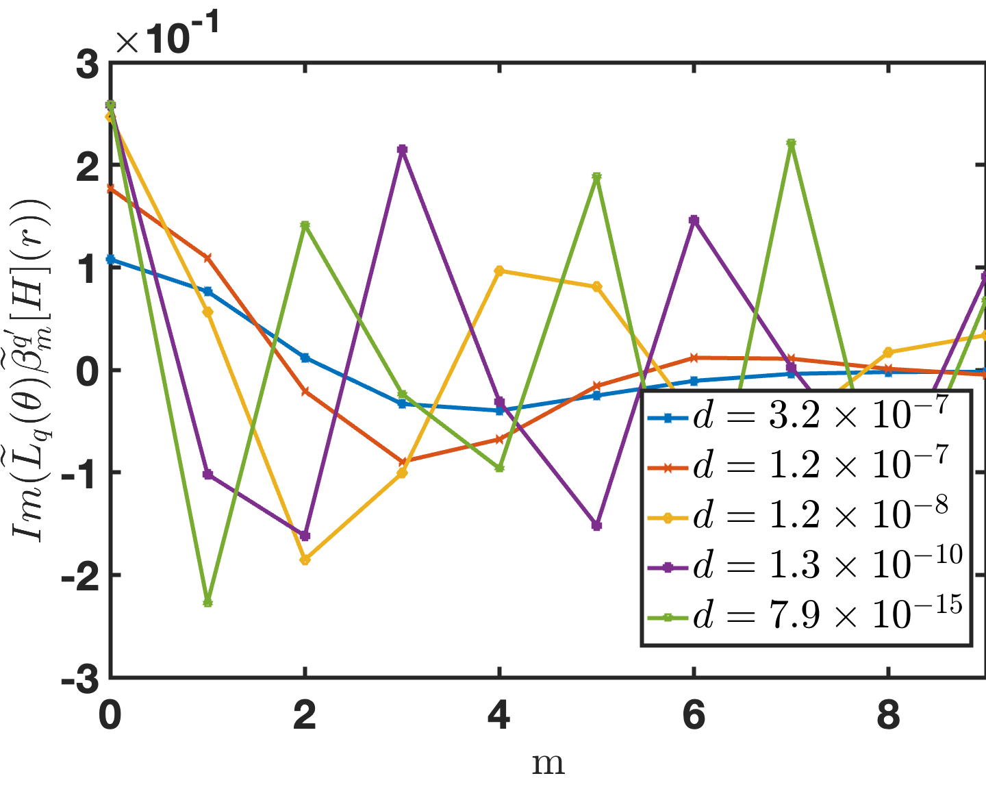
The rectangular-polar method introduced in Section 2.3 requires the precomputation of the integration weights in equation (26) for each one of the kernels , and , and for the singular and near-singular integration cases considered in Section 2.3, namely, for target points that are either within or close to the integration patch, respectively—and for which, in particular, the algorithm relies on the techniques introduced in the Section 3.3 for accurate computation of source-target distances. In previous implementations [12, 28] a change of variables was utilized as a singularity cancellation technique, upon which a high-order Fejér quadrature integration rule may be employed to precompute the integration weights with high accuracy. In the particular situation at hand, however, the kernel , which is actually bounded for at the corner and near the corner, still tends to infinity like , as illustrated in Figure 3, as both and approach the corner while maintains an angle bounded away from with the normal —a difficulty that is not shared by the kernels and , which tend to infinity only logarithmically and are thus natrually resolved by the rapid vanishing of the density as tends to the corner. (In contrast, the asymptotics of the normal-derivative kernel are not cancelled by the near vanishing of the density , where denotes the corner singularity exponent: as the distance from to the corner tends to zero.) As illustrated in Figure 3 (and as it is easy to appreciate by considering the geometry at hand), this peak corresponds to a different point in each case related both to the distance of the target point to the corner as well as the corner angle itself. Although, in principle, the location of this peak could be computed analytically and a similar additional singularity annihilating CoV could be incorporated to allow the successful use of Fejér quadrature for these scenarios as well, the implementation proposed in this paper relies instead on the adaptive Gauss-Kronrod (GK) quadrature scheme [18]. Since the GK scheme determines the optimal placement of integration points adaptively, this approach offers the advantage of simplicity (at the cost of a slight potential computational overhead and, in the current implementation, an error floor dictated by Matlab’s GK error limit; see Remark 1). Figure 4 displays values of precomputed integration weights; clearly, as suggested by the figure, the precomputed values are bounded quantities throughout the observation patch for all Chebyshev polynomial orders .
4 Numerical Results
This section illustrates the character and performance of the proposed algorithm by means of a variety of numerical results, including, 1) Quantitative evaluation of the algorithm’s performance as each one of the new key innovations is omitted (Section 4.1); 2) Evaluation of the conditioning of the linear systems and the numbers of GMRES iterations resulting from the proposed regularized R-CFIE formulation and comparison with the corresponding metrics resulting from the (unregularized) MFIE formulation (Section 4.2); 3) Convergence studies for computed field values at points extremely close to corners (Section 4.3); 4) Convergence studies for the integral density both near and away from corners (Section 4.4); and, 5) Evaluation of the singular exponent of the numerically computed solution density and comparison with the exponents based on theoretical considerations (Section 4.4). For uniformity, results of all such studies are presented for a cylindrical geometry with a square cross-section. To demonstrate the generality of the method, field convergence studies were conducted using scatterers of varying geometries, including parallelograms and teardrop-shaped objects with a wide range of interior angles. Specifically, the parallelograms included shapes with interior angles of and radians), while the teardrop-shaped scatterers feature curved boundaries with interior corner angles of and , respectively. All of the numerical errors reported in this section where obtained by means of the relative error expression
| (51) |
where denotes the maximum magnitude of the total field outside the scatterer. In all cases the reference solution was obtained as the numerical solution on a fine discretization, containing, in each case, at least twice as many discretization points as the finest discretization shown. Additionally, comparisons with solutions produced by a commercial solver are presented in Section 4.3 (Figure 14). All the results presented were obtained on the basis of Matlab implementation of the proposed algorithm running on an Apple Mac Mini M2 2023 personal computer. Computing times are not reported on account of the significant overhead associated with the Matlab implementation used. However, in view of the character of the algorithm it is expected that the computational cost required by an efficient implementation for a given number of discretization points should be similar to that obtained for related unaccelerated Nyström implementations [12, 28] for the same number of points, and they could of course be further accelerated by means of -type algorithmic acceleration of the type considered in [6] and references therein.
4.1 Quantitative Evaluation with Key Improvements Omitted
The scattering-solver algorithm for domains with corners described in previous sections relies on four main elements, namely, (i) The regularized integral formulation (29) and associated regularized integral equation (31) (which, while uniquely solvable, gives rise to unbounded densities and to integral kernels that are not weakly singular around corner points); (ii) The regularizing changes of variables (32), as described in Section 3.2; as well as, (iii) The change of unknown (42); and, (iv) The precision-preserving methodologies described in Section 3.3. In order to highlight the beneficial effects provided by these strategies, in this section we compare the performance of the proposed solver to the performance that results as one or more of the proposed techniques (ii), (iii) and (iv) are excluded from the proposed algorithm; the benefits arising from point (i) are then explored in Section 4.2.
In detail this section present numerical results obtained on the basis of the following formulations:
-
–
Original formulation: R-CFIE with all additional key improvements (ii), (iii) and (iv) omitted;
-
–
Intermediate formulation: R-CFIE formulation with the addition of the regularizing CoV mentioned in point (ii) above (without change of unknown) and incorporating additionally the precision-preserving methodologies mentioned in points (ii) and (iv);
-
–
Proposed formulation: R-CFIE formulation with the addition of the regularizing CoV, and the change of unknown and precision-preserving methodologies mentioned in points (ii)–(iv).
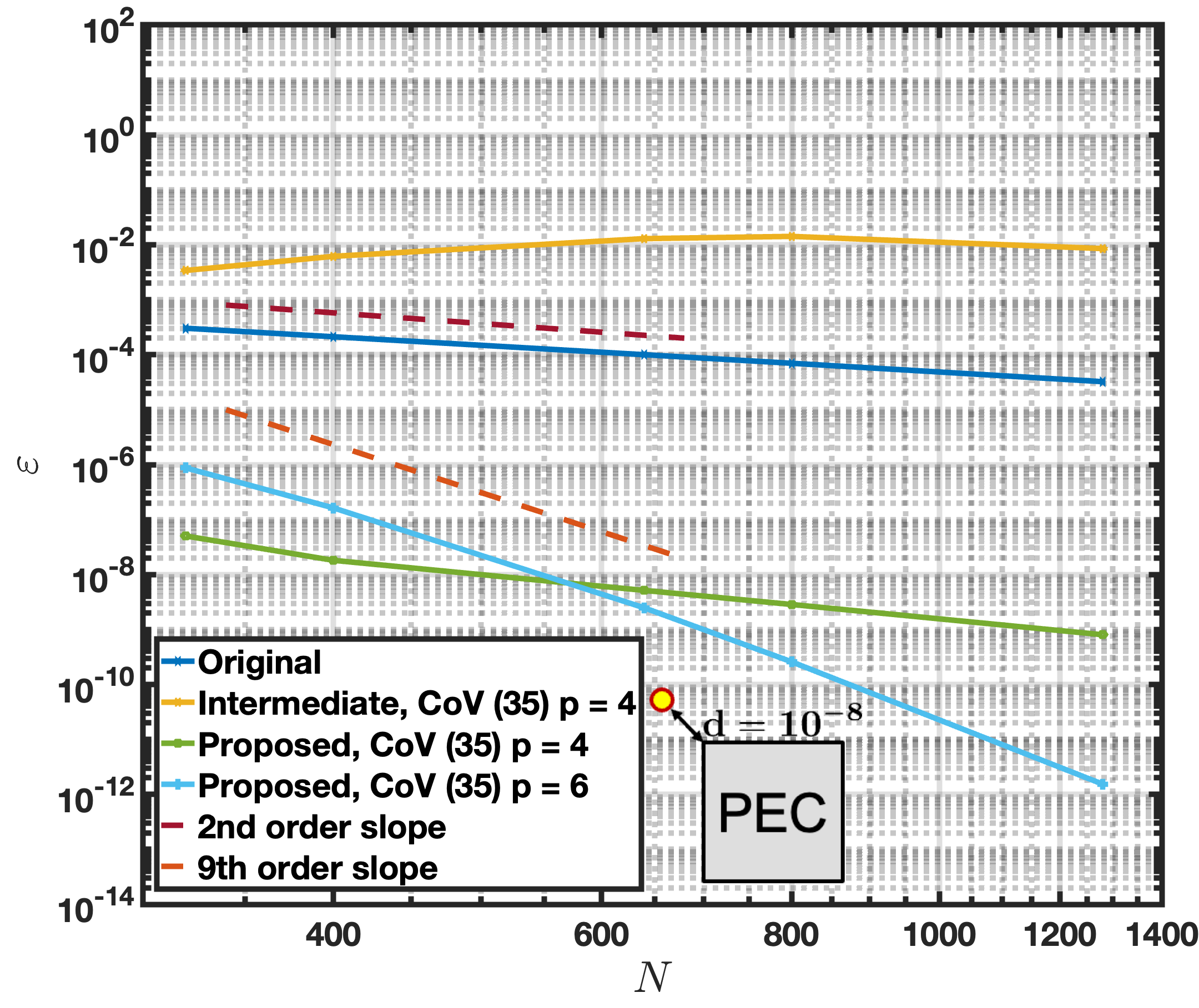
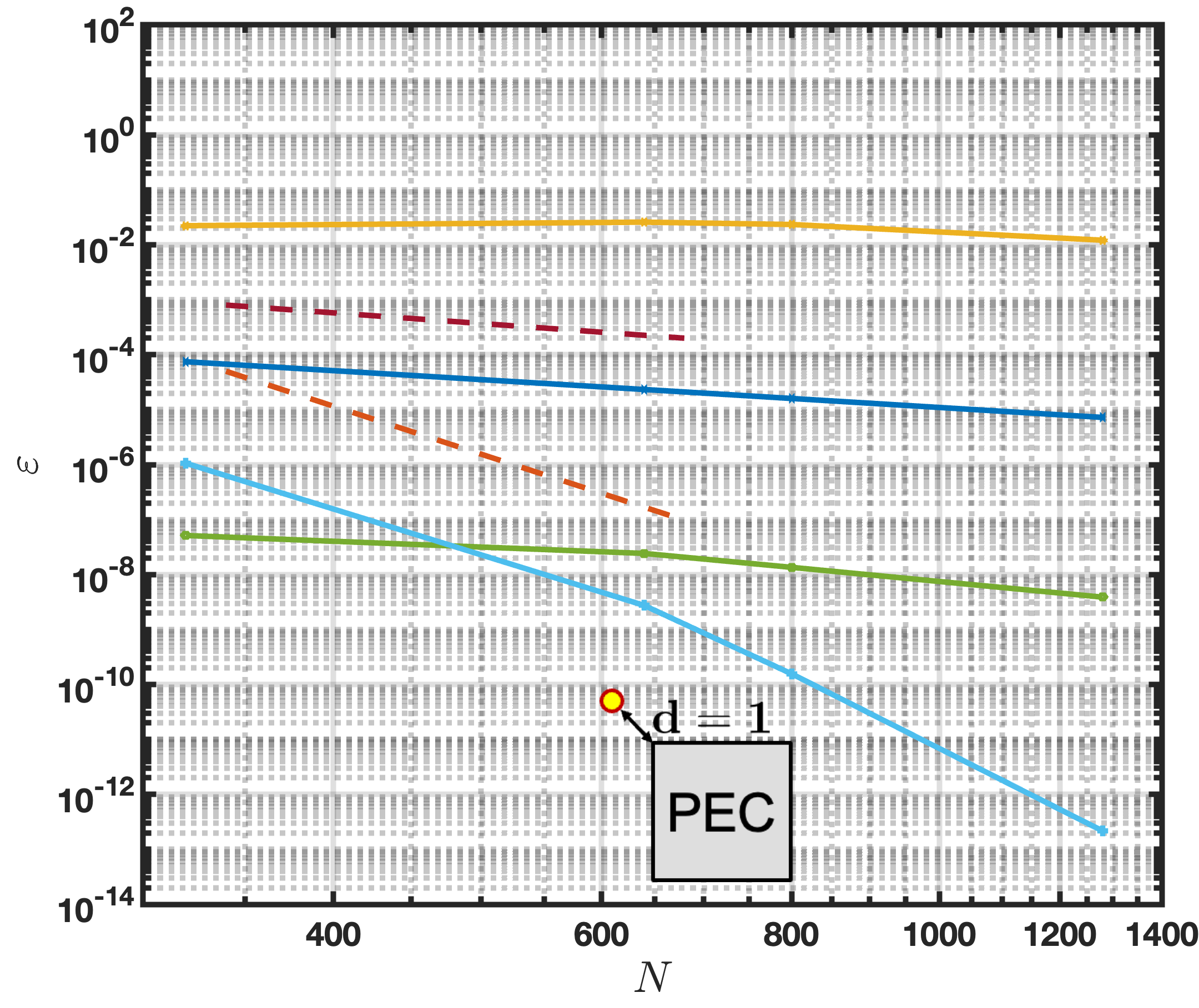
Figure 6 presents numerical convergence results obtained by means of each one of these formulations for the problem of scattering by a PEC cylinder with a square cross section of side that is illuminated by a plane wave excitation travelling in the positive direction, as depicted in Figure 5, with (that is and ). The scatterer is discretized into a finite number of patches, each one of which contains 10 discretization points. Error values at two points diagonally away from the top left corner of the scatterer are displayed in the figure, at distances (left) and (right) away from the corner, respectively, as indicated in the figure. The figure suggests that, as verified by means of observation points at varied distances, including much closer distances than the one cited above, the method is capable of producing high accuracies with similar numbers of discretization points both near and away from the corner point.
Remark 1.
The 12-digit accuracy limit depicted in Figure 6 and other error plots presented in this paper originates from the precision of the Gauss-Kronrod integration algorithm employed near corners, which is constrained to 12-digit accuracy in the Matlab implementation we have used. It is expected that use of a higher accuracy adaptive quadrature rule near corners would eliminate this limitation.
Figure 6 highlights the impact of each one the “key improvements” mentioned above in this section. Indeed, the figure illustrates the character of the proposed approach which, incorporating the Operator Regularized formuation, CoV, change of unknown, and precision preserving techniques (items (i) through (iv) above), achieves high-order convergence for any CoV degree—as illustrated in the figure for the CoV degrees and . In particular, the CoV results in an observed convergence rate faster than 9th order. The faster-than-expected convergence results from the high spectral accuracy achieved in patches away from corners. Notably, while these patches carry the dominant error in the examples considered, they still exhibit faster convergence compared to the error produced under the CoV around corners—as clearly illustrated in Figure 16 left in the numerical-results section. This observation suggests the potential for designing an error-balancing strategy that mitigates these two sources of error while reducing computational costs for a given error tolerance. However, for the sake of simplicity, it may be reasonable to accept a limited degree of suboptimality in exchange for a more straightforward algorithmic design.
Next, we examine the algorithms that arise when some or all of the key improvements are not included. The original method (including point (i) but excluding point (ii), and therefore excluding points (iii) and (iv) which are rendered irrelevant in absence of point (ii)) only achieves second order convergence, on account of the corner singular character of the integral density. The Intermediate algorithm, which omits the change of unknown strategy (point (iii)), performs worse than the original approach, emphasizing the significant impact inherent in this important algorithmic strategy. The precision-preserving strategies mentioned in point (iv) are important for any approaches using a CoV, since the CoV causes the discretization points to cluster so close to the corners that values of the source-target difference exactly vanishes numerically for certain , thus giving rise to runtime errors at significant numbers of discretization points.
4.2 Conditioning and Number of GMRES Iterations
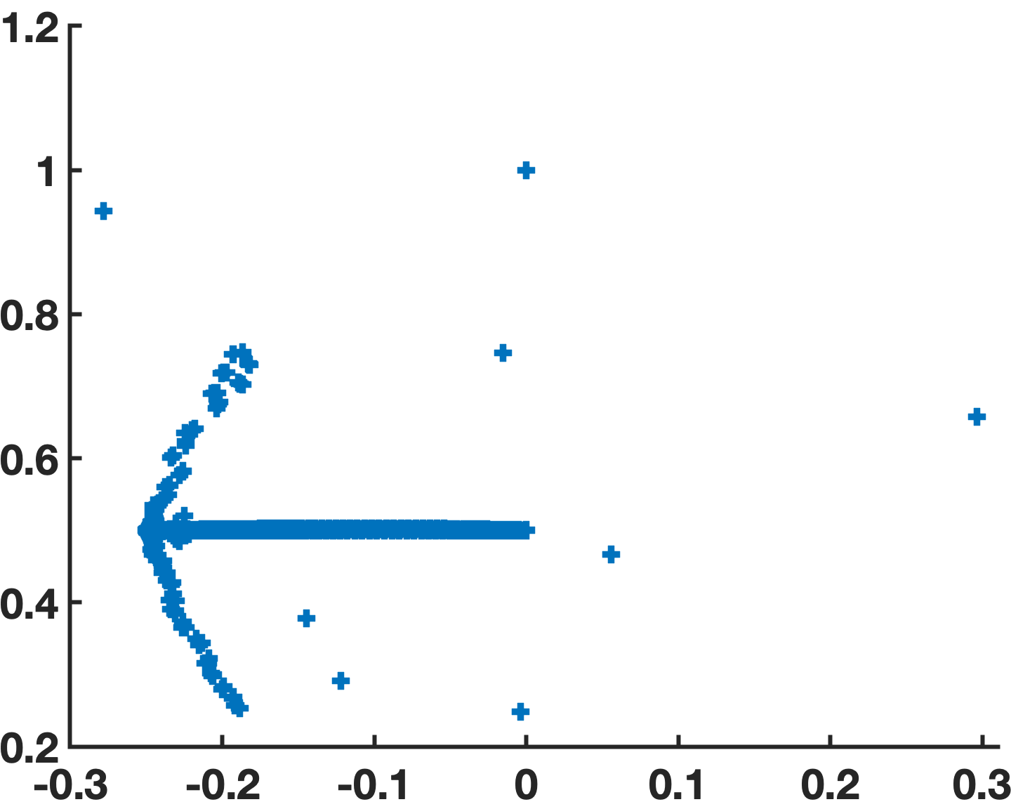
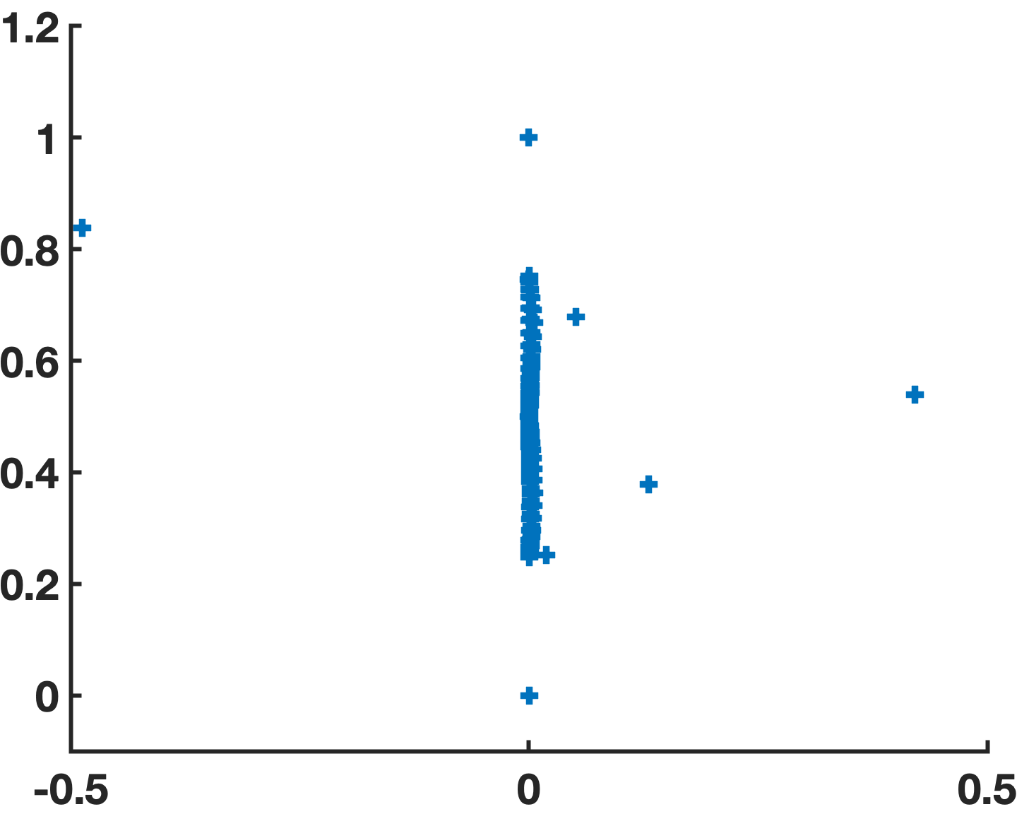
In order to highlight the attractive linear-algebra conditioning properties resulting from the proposed corner-capable CFIE-R regularized combined formulation, we compare it in this section with the corresponding MFIE formulation—using, in both cases, all of the key improvements (i) through (iv) in Section (4.1). In order to do this in a controlled manner, we consider once again the problem of scattering by a square cylinder of side , for which the interior Laplace resonances can be computed in closed form:
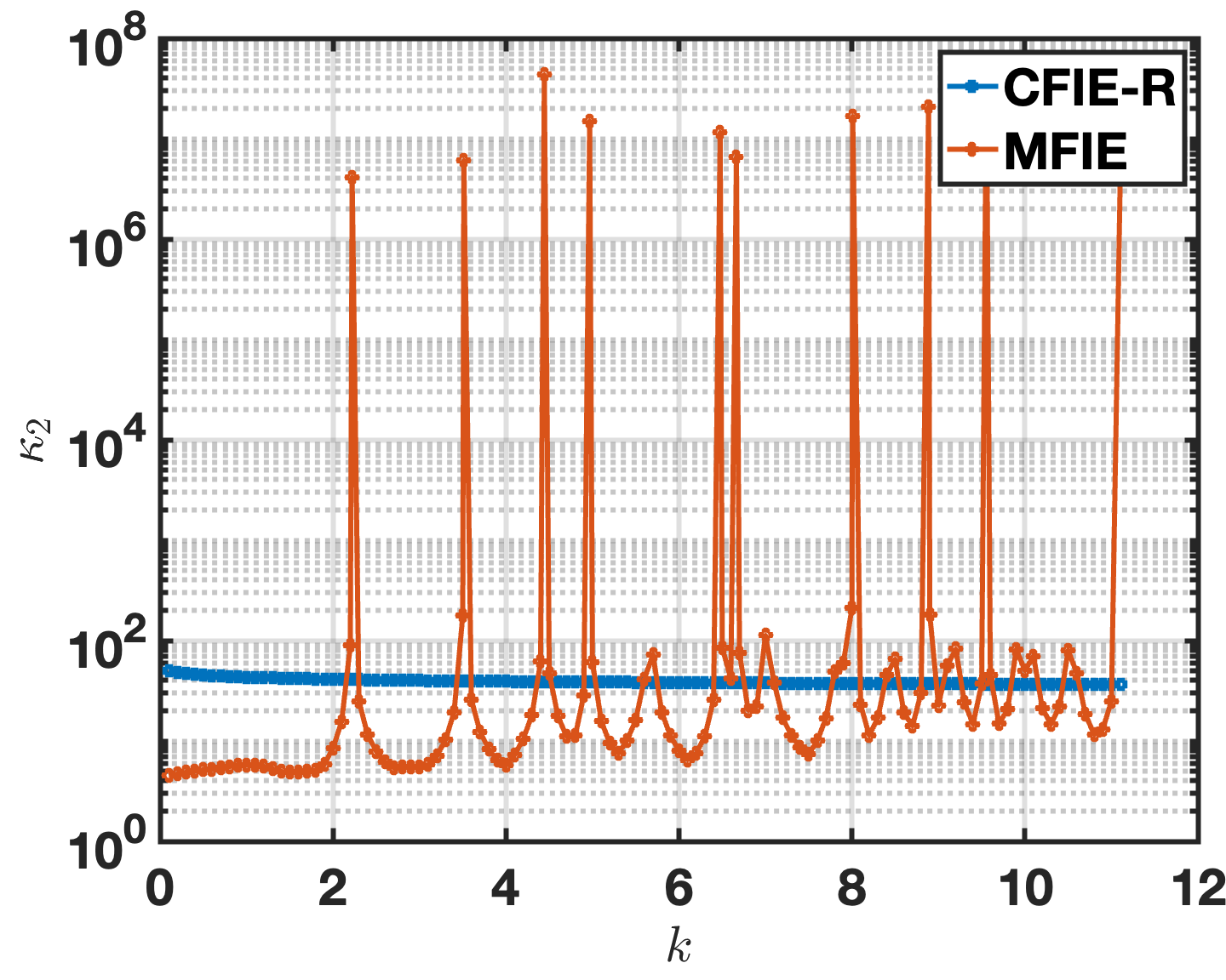
for all positive integer values of and . We thus consider the BIE systems for and, to visualize the singularity/non-singularity of the associated MFIE/CFIE-R matrix equations, we present in Figure 7 (left for MFIE and right for CFIE-R) the corresponding eigenvalue distributions. In particular, we see that the MFIE system is singular: is an eigenvalue. At the same wavenumber, in contrast, the eigenvalues of the CFIE-R system are all non-zero. Figure 8 left, which displays the condition numbers vs. wavenumber for the MFIE and CFIE-R formulations, shows significant condition-number spikes for the MFIE formulation at each of the resonances corresponding to the cavity modes of the square cylinder while remaining bounded for the CFIE-R formuilation—thus indirectly demonstrating the resonance-free/singular character of the CFIE-R/MFIE formulations considered.
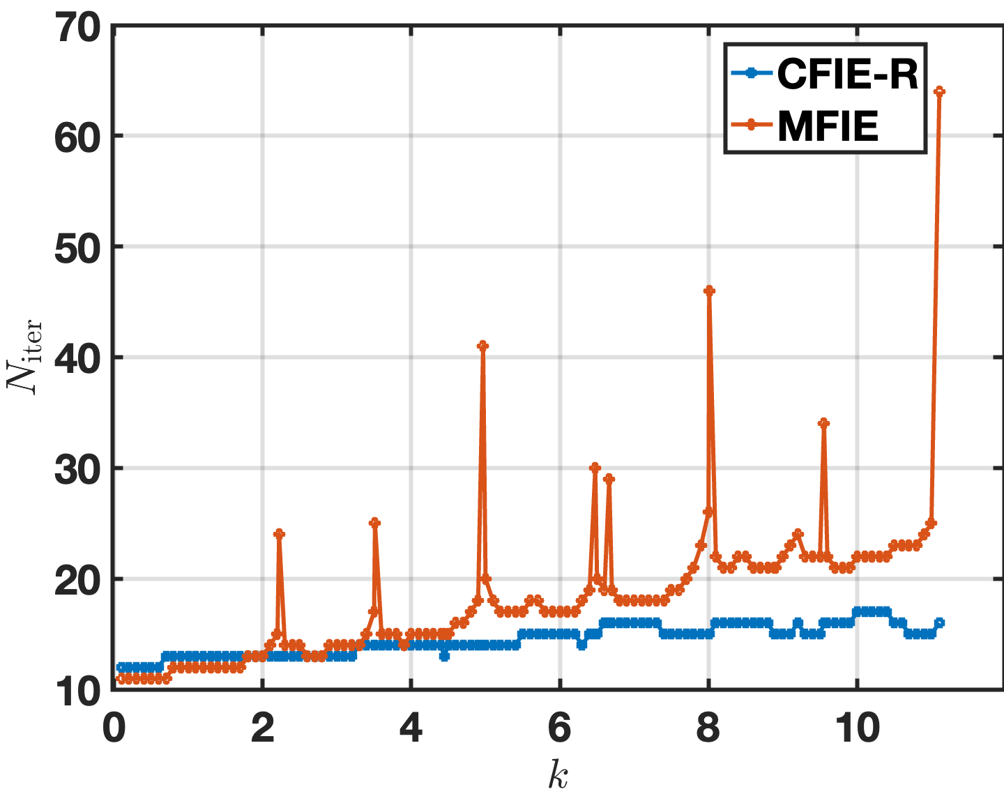
Figure 8 right presents the number of iterations required by the GMRES iterative algorithm to achieve a residual of vs. wavenumber for both the MFIE and CFIE-R. It can be seen that the CFIE-R system achieves the prescribed tolerance for all wavenumbers considered in less than 15 iterations, growing only moderately with the wavenumber, while the number of iterations required to solve the MFIE spikes near each resonance and grows steadily even away from the resonances. This highlights the favorable iteration numbers and resonance-free properties of the proposed CFIE-R corner regularized formulation. We expect that the favorable number of iterations of the CFIE-R formulation will be crucial in the 3D case where iterative solvers become a necessity for large problems.
4.3 Field evaluation accuracy
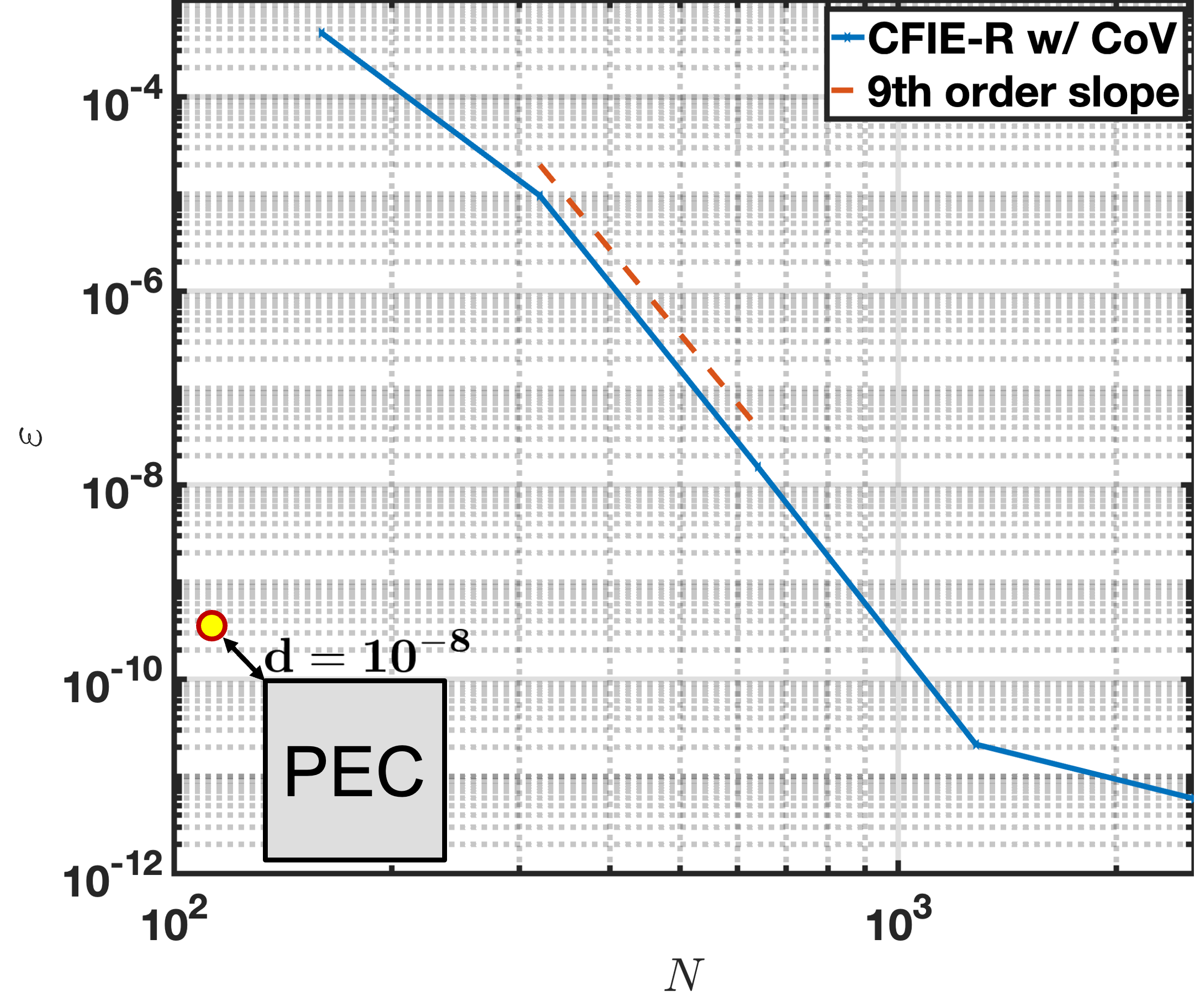
In this section, the accuracy of the proposed method with all of the key improvements incorporated is evaluated for several different geometries and excitations. The first example considered is a PEC cylinder with square cross-section of sidelength with a monopole point source excitation located within the scatterer. Due to the PEC nature of the object (under the boundary conditions (2)), the resulting scattered field outside the scatterer equals the negative of the incident monopole field. Thus, the incident field can be used to determine the accuracy of the scattered field. Figure 9 plots the convergence of the corner-regularized CFIE-R with CoV order vs. number of unknowns of evaluating the field at a point that is a distance away diagonally from the top left corner of the square cylinder. Errors smaller than are obtained with a 9th-order convergence slope.
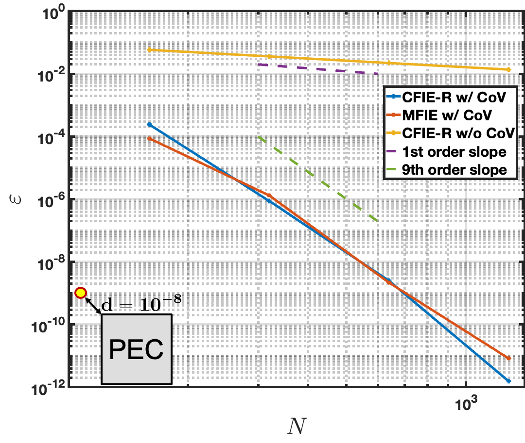
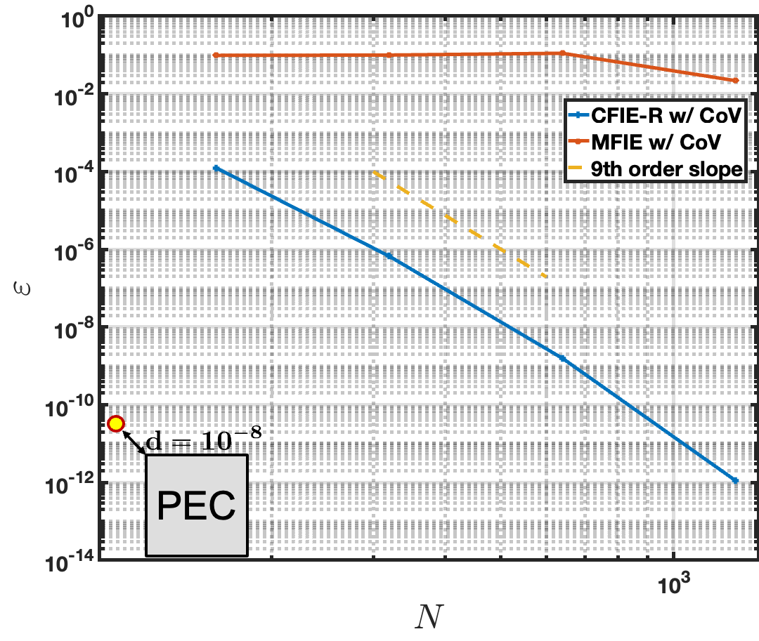
For the next example, the scattering from the same square cross-section cylinder is considered with the planewave incident excitation illustrated in Figure 5. This example compares the performance of the corner-regularized MFIE and CFIE-R formulations at wavenumbers and , the second of which is very close to a resonance of the MFIE. A CoV of order is used in all cases except for a curve “w/o” CoV. Figure 10 left illustrates the convergence behavior of the field produced by the corner-regularized MFIE and CFIE-R formulations at a point diagonally offset from the top-left corner of the scatterer, with a wavenumber . Both the MFIE and CFIE-R produce similar accuracies when the wavenumber is not near an MFIE resonance, achieving a relative error of and 9-th order convergence. For comparison, the convergence of the CFIE-R without a change of variables (CoV) is also plotted, demonstrating the expected first-order convergence caused by the corner singularity, with errors that remain larger than even for discretizations containing over 1000 unknowns. Figure 10 right plots the convergence of the field evaluation at the same point for the wavenumber is , which is very close to a resonance of the MFIE operator. In this scenario, the CFIE-R exhibits convergence nearly identical to that observed for . However, the MFIE fails entirely, producing inaccurate results regardless of the number of unknowns used.
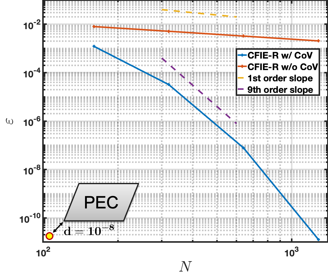
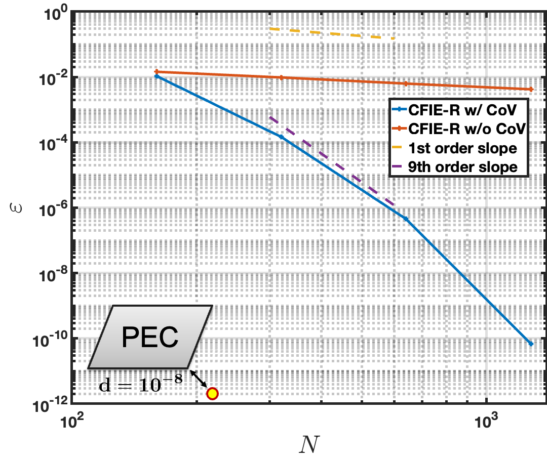
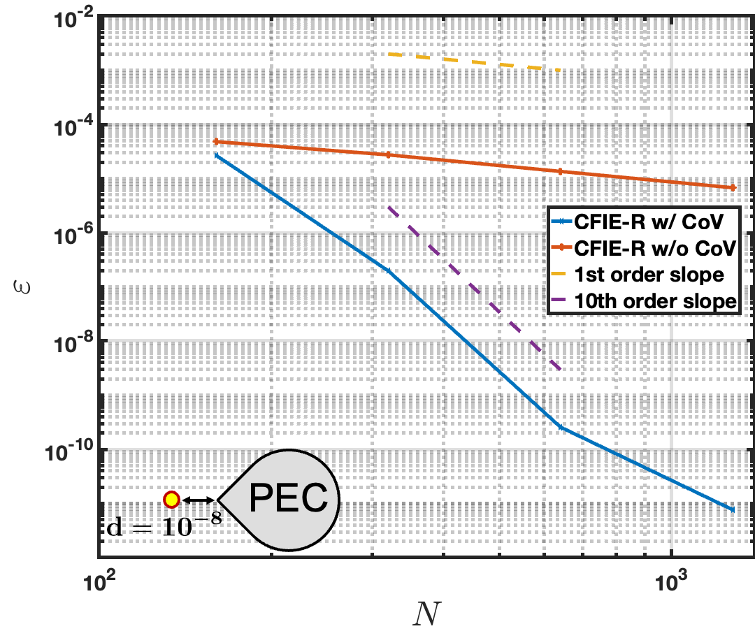
The next two examples examine the field convergence of the proposed method for scatterers different from the square cross-section cylinders considered up to this point, namely, cylinders with parallelogram ( acute angle) and teardrop-shaped cross-sections. (The parallelogram has sides of lengths and .) The field convergence is evaluated at a point diagonally offset from the bottom-left and bottom-right corners in Figure 11 left and right, which have interior angles of and , respectively. The results indicate that the corner-regularized CFIE-R with a CoV order of achieves similar convergence near both corners, despite their differing interior angles, attaining better than 9th-order convergence and a relative error below . This performance resembles closely those observed for the square cross-section examples. In contrast, the original rectangular polar method without CoV provides first-order convergence only, and it fails to achieve even two digits of accuracy.
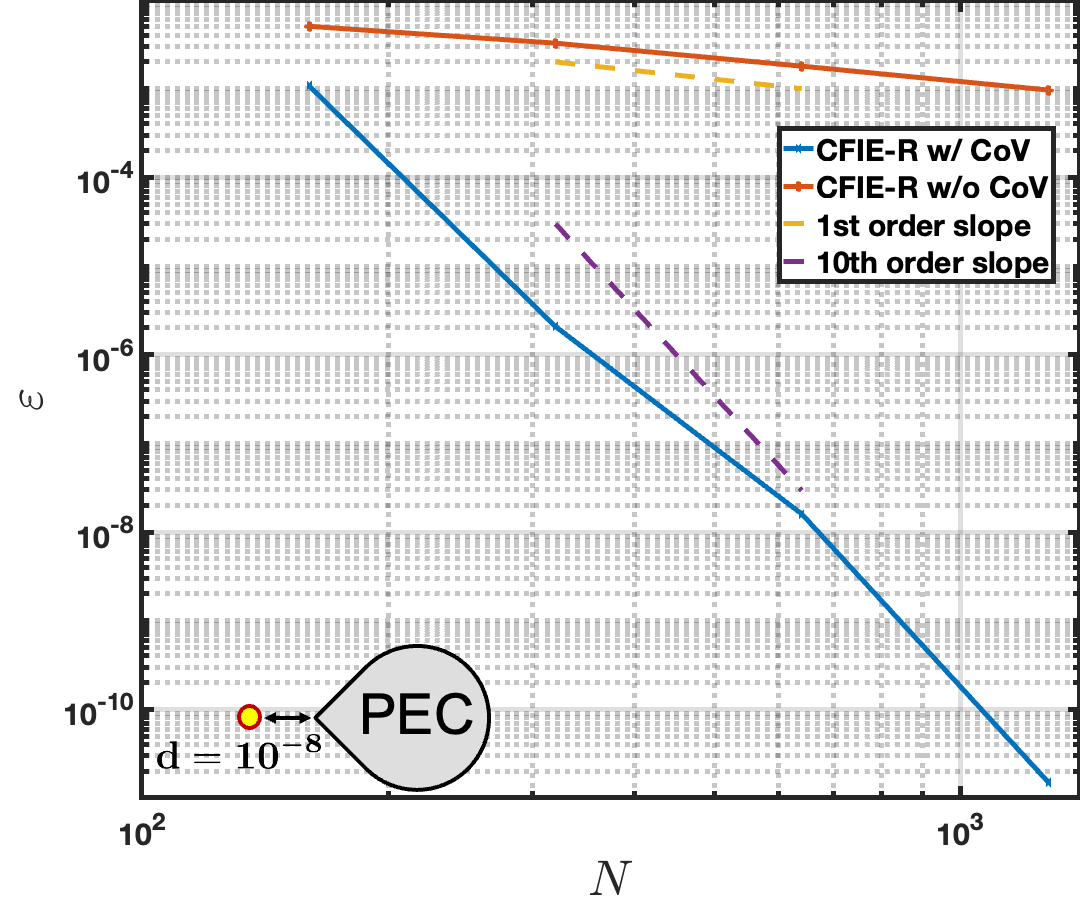
The “teardrop” shaped geometry
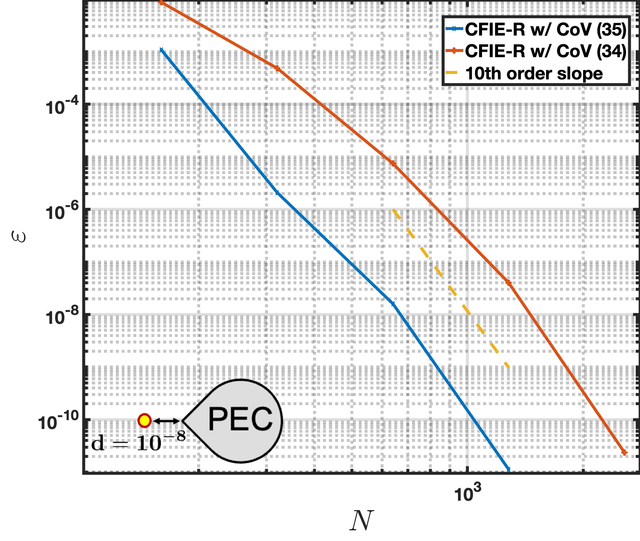
is considered next where the parameter controls the angle of the corner; values resulting interior angles of and are considered in what follows. Figure 12 left illustrates the convergence of the field evaluated at a point located a distance diagonally from the teardrop corner, showing that the CoV order of yields 10th-order convergence with a relative error below , demonstrating once again higher than expected convergence on account of over-resolution of the corner. In contrast, the original RP method (44) exhibits only linear convergence, achieving fewer than three digits of accuracy even with more than 1000 unknowns. Figure 12 right compares, for the teardrop scatterer, the performance resulting from use CoVs (32) and (34). While both CoV functions achieve similar best-case accuracy and convergence rates in field evaluation, the CoV (32) proves significantly more efficient, delivering a solution that is up to three digits more accurate for the same number of unknowns. This superior performance is attributed to the uneven distribution of discretization points it produces along the domain boundary, as discussed in Section 3.2.
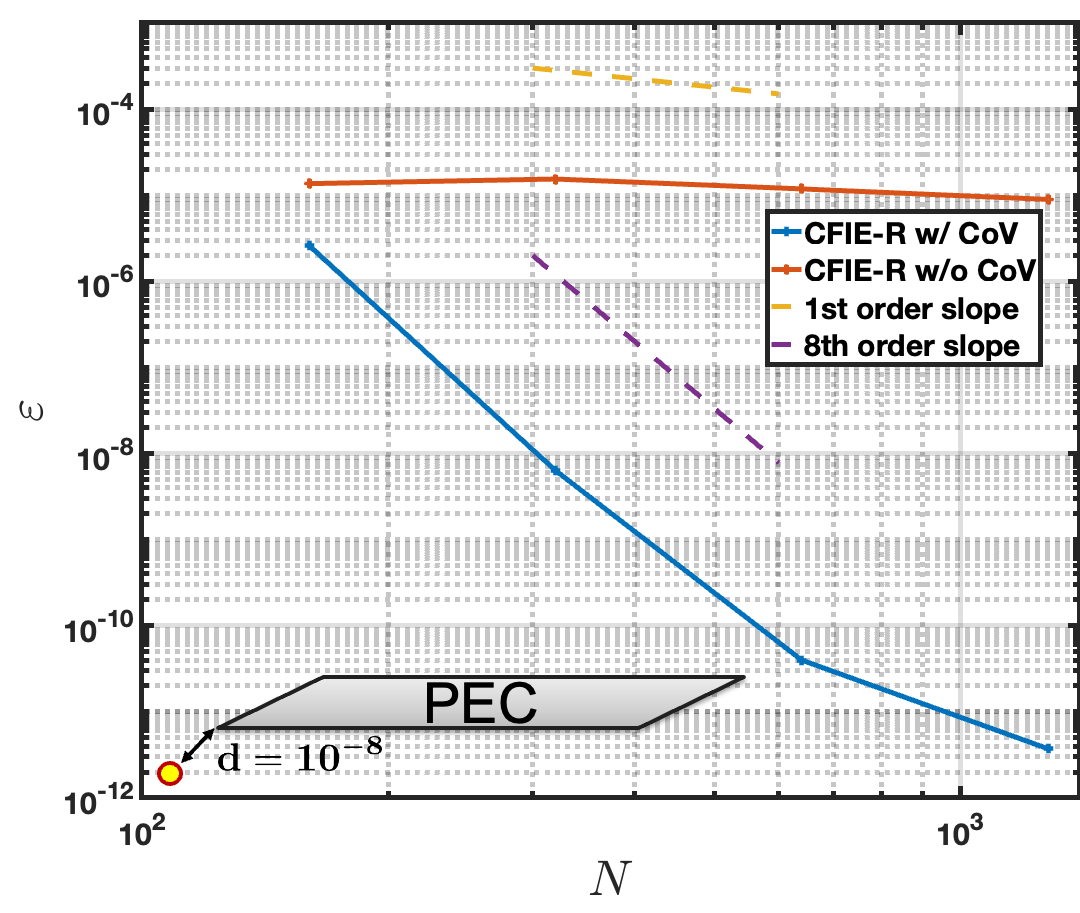
The proposed methods consistently maintain accuracy across a wide range of corner angles, as illustrated in what follows for a teardrop and a “needle-like” parallelogram with an acute angle of approximately radians). In both cases, the relative error in the field evaluation is plotted for a point at a distance diagonally offset from the corner, as shown in Figure 13. The results demonstrate that the corner-regularized CFIE-R with a CoV order of achieves a relative error of approximately in both cases, with 10th-order convergence for the small-angle teardrop and 8th-order convergence for the needle-like parallelogram. In contrast, the original RP method for solving the CFIE-R system fails to achieve more than three digits of accuracy and exhibits only linear convergence in both cases.
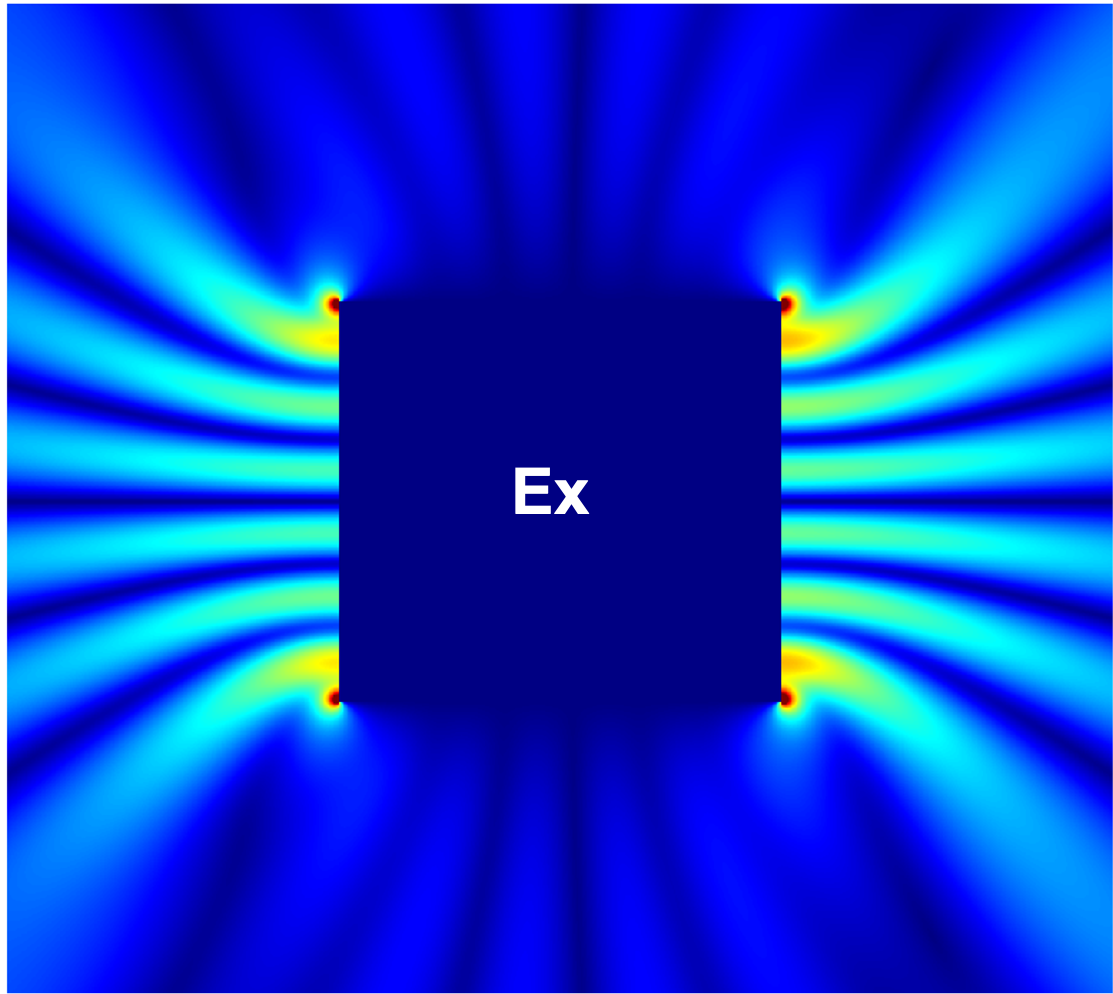
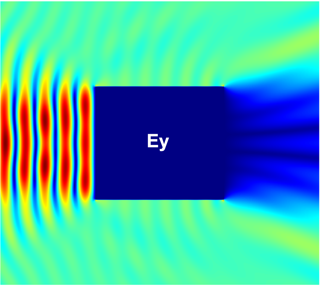
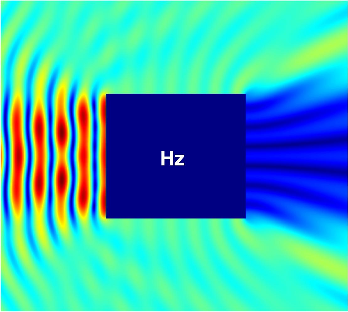
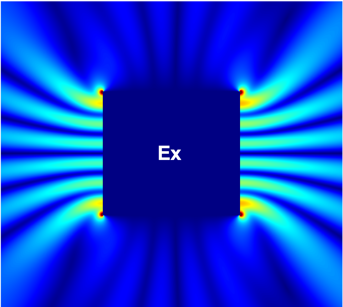
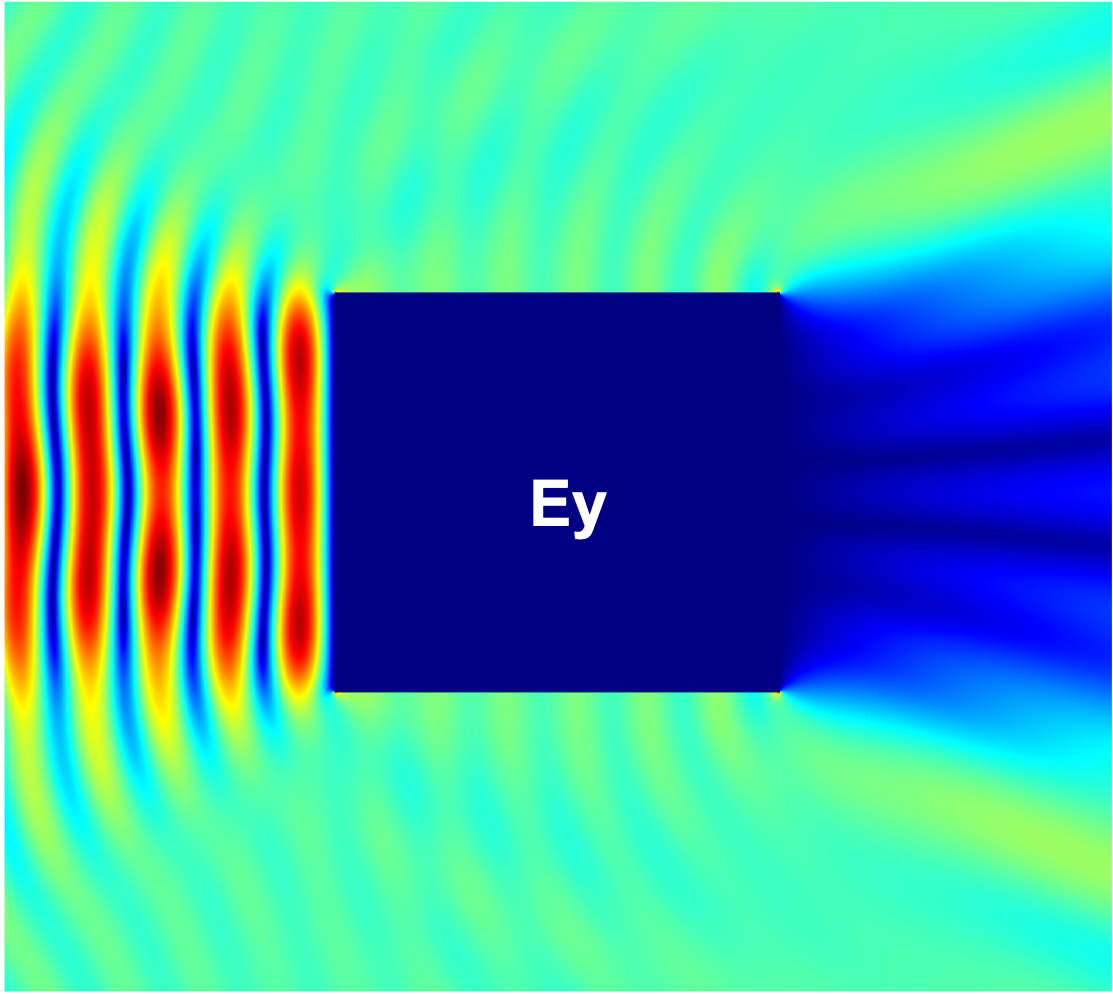
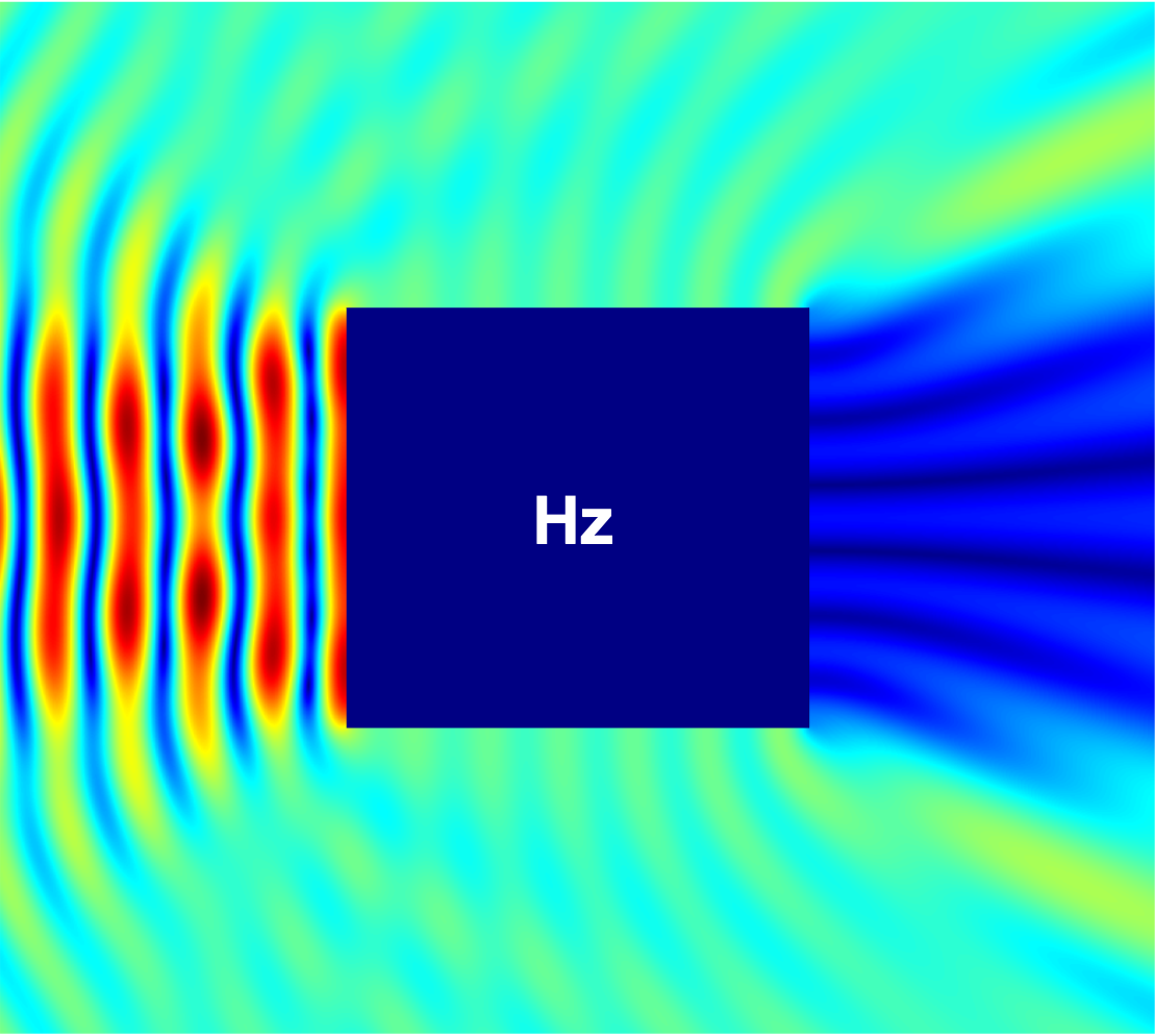
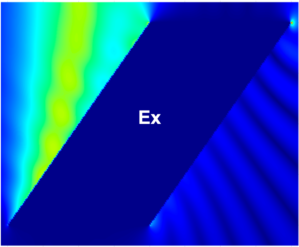
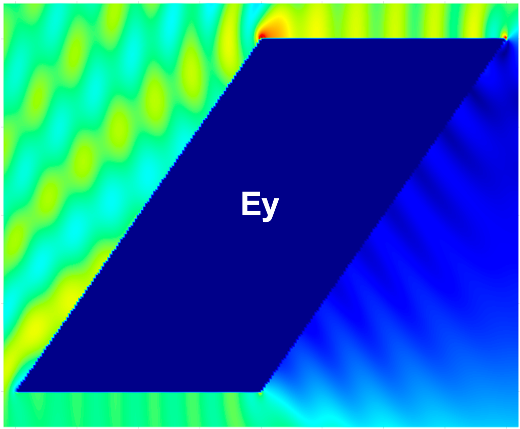
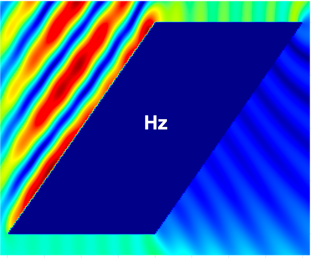
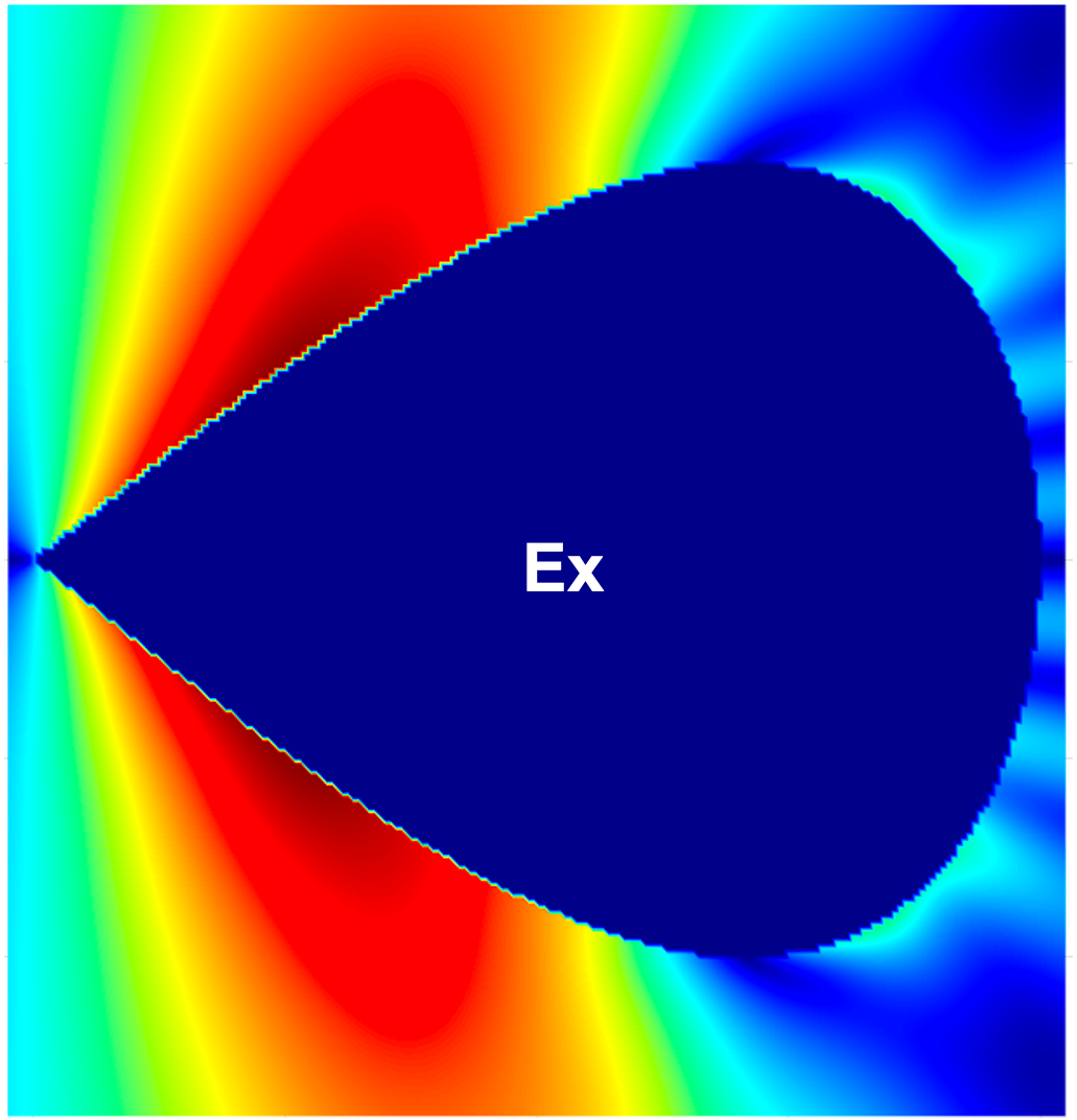
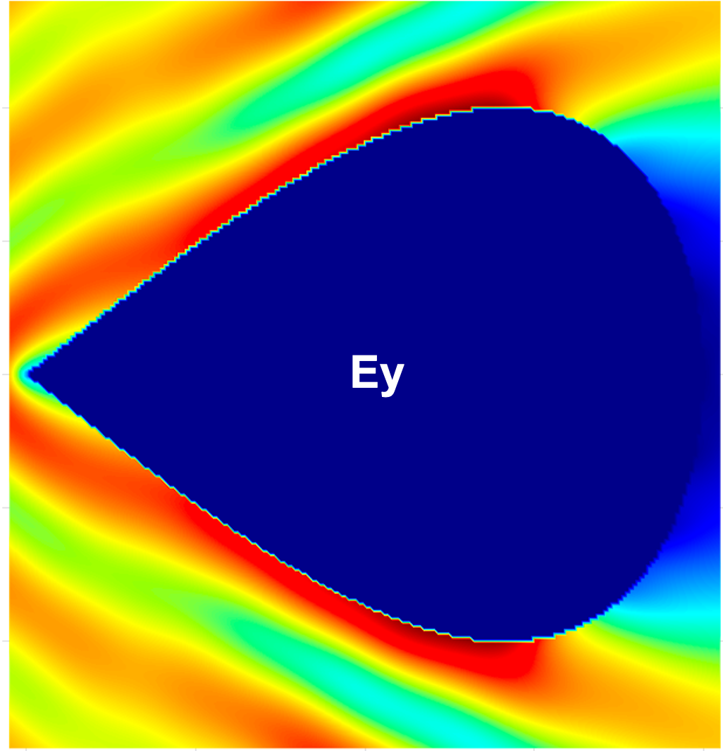
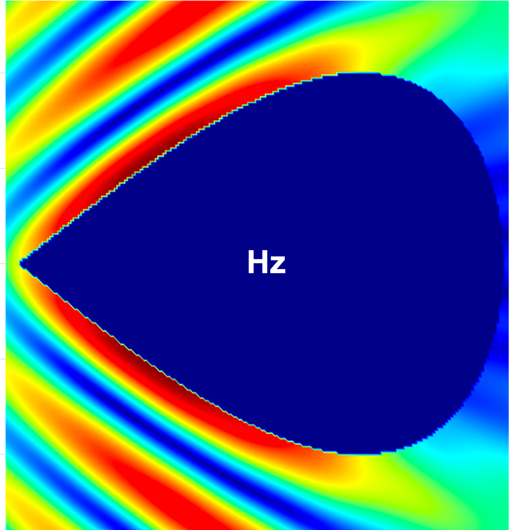
Figure 14 compares the magnitudes of the total field components , , and within a region for the PEC cylinder with a square cross-section excited with a planewave with , computed using the proposed method and the commercial FDTD solver Lumerical with an extremely fine mesh ( maximum grid step size). The results show excellent agreement, validating the correctness of the proposed method. igure 15 additionally presents the magnitudes of the total field components , , and for the parallelogram with a interior angle and the teardrop with a interior angle examples considered above in this section.
4.4 Density errors and density corner-exponent evaluation
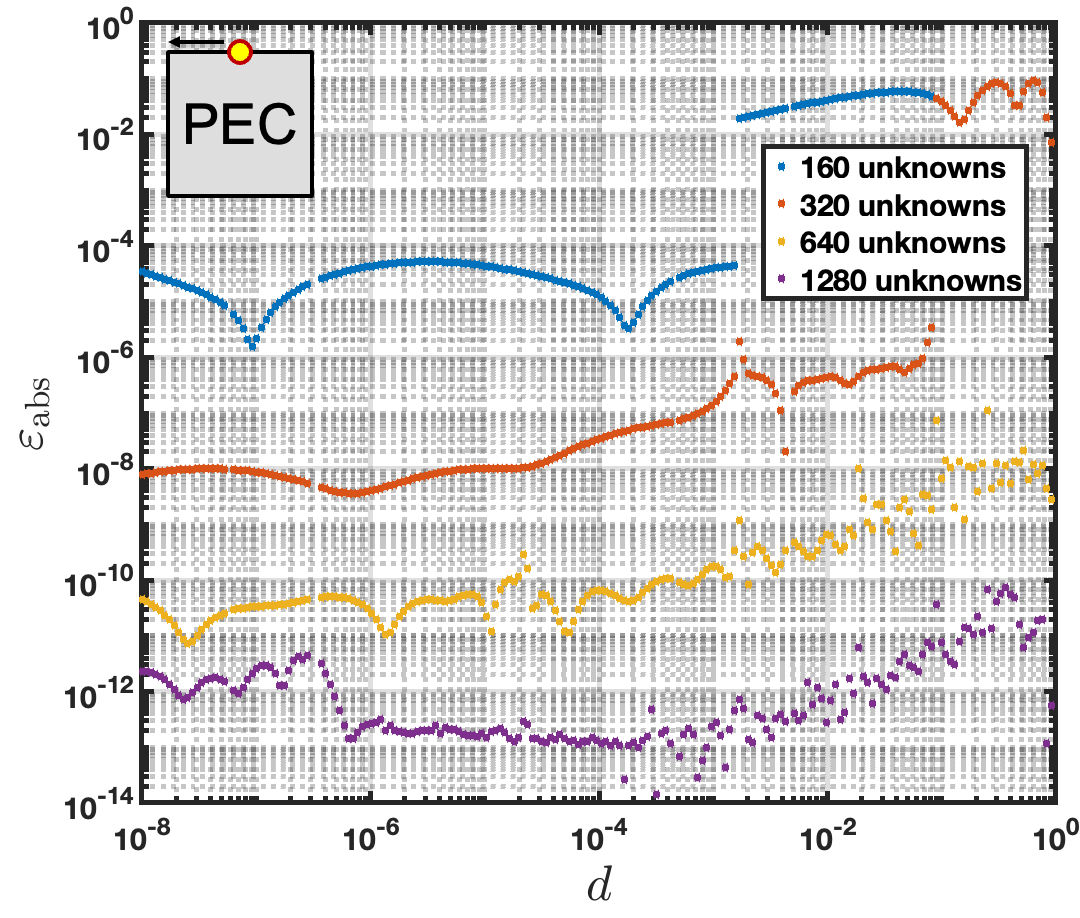
This section considers the accuracy obtained for the density solution introduced in (42) at points both near and away from a corner. The square cross-section PEC cylinder with sidelength and planewave excitation as in Figure 5 are used for this illustration. Figure 16 left displays the absolute error in vs. distance from the corner for the top horizontal boundary of the square. As expected, the error decreases as the number of unknowns used to discretize the geometry is increased. As discussed in Section 4.1, for the coarser discretizations the error near the corner is significantly lower than away from the corner. As dicussed in that section, the errors decrease more slowly near the corner as the discretizations are refined, which implies that the overall solution error is limited by that near the center of the boundary for the coarser discretizations—which explains the near 10-th order rate of convergence observed in some cases in spite of the lower order CoV used. The method achieves density absolute errors lower than for evaluation points away from a corner.
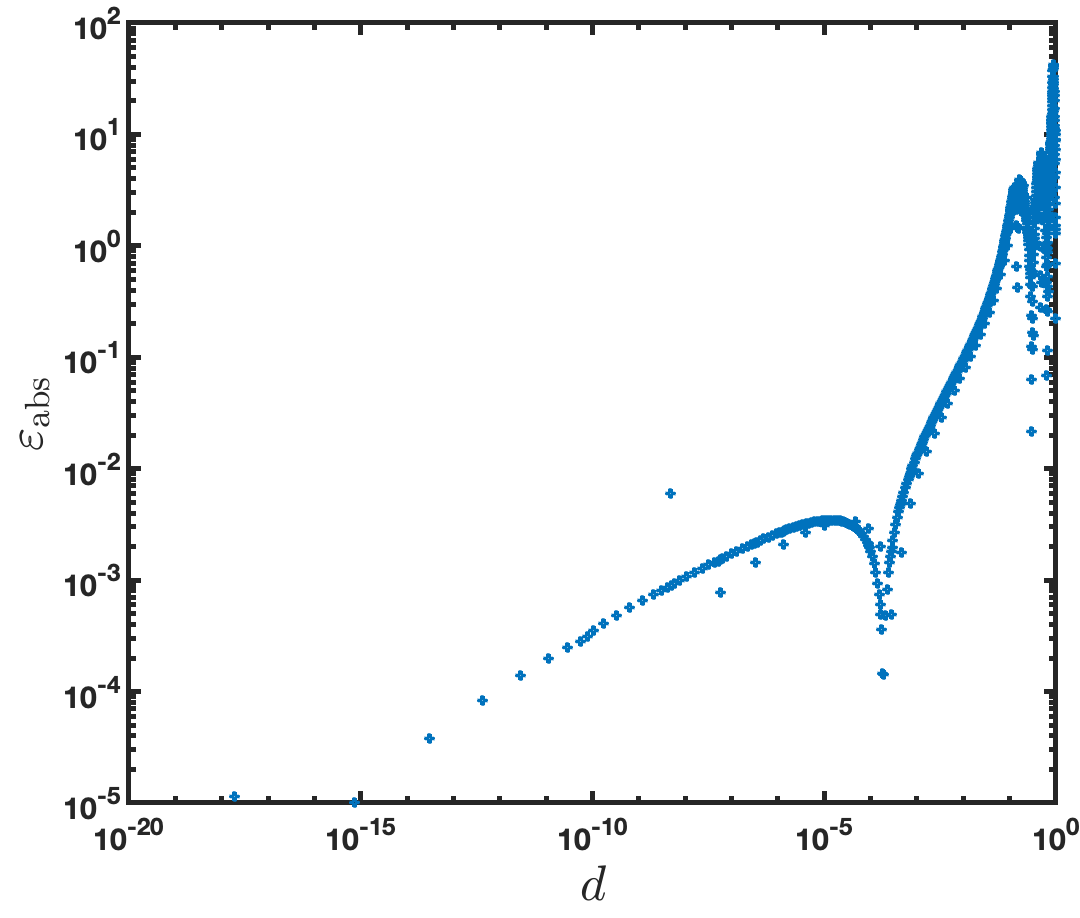
It is interesting to additionally consider the asymptotic behavior of the the CFIE-R density in (31) that may be obtained numerically by division from the density in (42). For a interior angle, the density at a Cartesian distance from the corner, which is denoted by in what follows, tends to infinity like , with , as [14]. The exponent can be extracted from the numerical solution as the limit of the slope of a log-log plot of the density at the distance from the corner, as a function of . The slope is given by
| (52) |
Figure 16(b), which plots vs. the distance from the corner , shows that indeed, as : the precision of the numerical solution suffices to produce the singular exponent in the density with an accuracy of at least 8 digits.
5 Conclusions
This contribution introduced and validated a novel formulation and discretization strategy for the solution of problems of electromagnetic scattering by objects containing geometric singularities. The proposed method achieves high-order convergence, comparable to that obtainable by related Nyström methods for smooth geometries, even for field evaluations at points extremely close to corners, and even for extremely sharp, needle-like corner angles. Building on the well-conditioned, resonance-free regularized CFIE-R formulation [11], the approach incorporates a corner-regularization technique that combines a polynomial-like change of variables (CoV) with an associated change of unknown. By incorporating the vanishing line element from the CoV directly into the unknown this reformulation ensures smooth behavior of the new unknown near corners. Using additionally several precision-preserving techniques to address the challenges posed by CoV-related clustering of points near the corners, the method results in fast convergence and high accuracies in the restuling scattered field, at distances both close and far from the scatterer’s corners.
Extensive numerical results confirm the unique solvability, resonance-free character, and high-order convergence of the proposed approach for various geometries, including corners with very small interior angles. In most cases, the method achieves a relative error near with faster than 9th-order convergence for field evaluations at arbitrary distances from a corner. Total field magnitudes outside the scatterers are plotted for several geometries demonstrating excellent agreement with results obtained from a commercial FDTD solver.
In conclusion, the proposed methodology represents a significant advancement in the numerical modeling of electromagnetic scattering problems. It offers a robust, efficient, and highly accurate solution framework, particularly for scatterers with geometric corner singularities. This approach establishes a strong foundation for future extensions to three-dimensional Maxwell scattering problems for scatterers containing corners and edges.
Acknowledgments
The authors gratefully acknowledge support by the Air Force Office of Scientific Research (FA9550-20-1-0087, FA9550-25-1-0020, FA9550-21-1-0373 and FA9550-25-1-0015) and the National Science Foundation (CCF-2047433 and DMS-2109831).
References
- [1] Anand, A., Ovall, J. S., and Turc, C. Well-conditioned boundary integral equations for two-dimensional sound-hard scattering problems in domains with corners. The Journal of Integral Equations and Applications (2012), 321–358.
- [2] Atkinson, K. E. The numerical solution of integral equations of the second kind, vol. 4. Cambridge university press, 1997.
- [3] Atkinson, K. E., and Graham, I. G. An iterative variant of the Nyström method for boundary integral equations on nonsmooth boundaries. The mathematics of finite elements and applications, VI (Uxbridge, 1987), London (1988), 297–303.
- [4] Babuška, I., Kellogg, R. B., and Pitkäranta, J. Direct and inverse error estimates for finite elements with mesh refinements. Numerische Mathematik 33, 4 (1979), 447–471.
- [5] Babuška, I., and Miller, A. The post-processing approach in the finite element method—part 2: the calculation of stress intensity factors. International Journal for Numerical Methods in Engineering 20, 6 (1984), 1111–1129.
- [6] Bauinger, C., and Bruno, O. P. “Interpolated Factored Green Function” method for accelerated solution of scattering problems. Journal of Computational Physics 430 (2021), 110095.
- [7] Bleszynski, E., Bleszynski, M., and Jaroszewicz, T. AIM: Adaptive integral method for solving large-scale electromagnetic scattering and radiation problems. Radio Science 31, 5 (1996), 1225–1251.
- [8] Boyd, J. P. Chebyshev and Fourier spectral methods. Courier Corporation, 2001.
- [9] Bremer, J. A fast direct solver for the integral equations of scattering theory on planar curves with corners. Journal of Computational Physics 231, 4 (2012), 1879–1899.
- [10] Bruno, O. P., Elling, T., Paffenroth, R., and Turc, C. Electromagnetic integral equations requiring small numbers of krylov-subspace iterations. Journal of Computational Physics 228, 17 (2009), 6169–6183.
- [11] Bruno, O. P., Elling, T., and Turc, C. Regularized integral equations and fast high-order solvers for sound-hard acoustic scattering problems. International Journal for Numerical Methods in Engineering 91, 10 (2012), 1045–1072.
- [12] Bruno, O. P., and Garza, E. A Chebyshev-based rectangular-polar integral solver for scattering by geometries described by non-overlapping patches. Journal of Computational Physics 421 (2020), 109740.
- [13] Bruno, O. P., and Kunyansky, L. A. A fast, high-order algorithm for the solution of surface scattering problems: basic implementation, tests, and applications. Journal of Computational Physics 169, 1 (2001), 80–110.
- [14] Bruno, O. P., Ovall, J. S., and Turc, C. A high-order integral algorithm for highly singular pde solutions in lipschitz domains. Computing 84 (2009), 149–181.
- [15] Cheng, H., Crutchfield, W. Y., Gimbutas, Z., Greengard, L. F., Ethridge, J. F., Huang, J., Rokhlin, V., Yarvin, N., and Zhao, J. A wideband fast multipole method for the Helmholtz equation in three dimensions. Journal of Computational Physics 216, 1 (2006), 300–325.
- [16] Colton, D. Inverse acoustic and electromagnetic scattering theory, 1998.
- [17] Cox, C. L., and Fix, G. J. On the accuracy of least squares methods in the presence of corner singularities. Computers & mathematics with applications 10, 6 (1984), 463–475.
- [18] Davis, P. J., and Rabinowitz, P. Methods of numerical integration. Courier Corporation, 2007.
- [19] Demkowicz, L., Devloo, P., and Oden, J. T. On an -type mesh-refinement strategy based on minimization of interpolation errors. Computer Methods in Applied Mechanics and Engineering 53, 1 (1985), 67–89.
- [20] Devloo, P. Recursive elements, an inexpensive solution process for resolving point singularities in elliptic problems. In Proceedings of 2nd World Congress on Computational Mechanics. IACM, Stuttgart (1990), pp. 609–612.
- [21] Fix, G. J., Gulati, S., and Wakoff, G. On the use of singular functions with finite element approximations. Journal of Computational Physics 13, 2 (1973), 209–228.
- [22] Ganesh, M., and Graham, I. G. A high-order algorithm for obstacle scattering in three dimensions. Journal of Computational Physics 198, 1 (2004), 211–242.
- [23] Givoli, D., Rivkin, L., and Keller, J. B. A finite element method for domains with corners. International journal for numerical methods in engineering 35, 6 (1992), 1329–1345.
- [24] Graham, I., and Chandler, G. High-order methods for linear functionals of solutions of second kind integral equations. SIAM journal on numerical analysis 25, 5 (1988), 1118–1137.
- [25] Graham, I., and Chandler, G. High-order methods for linear functionals of solutions of second kind integral equations. SIAM journal on numerical analysis 25, 5 (1988), 1118–1137.
- [26] Helsing, J. Solving integral equations on piecewise smooth boundaries using the RCIP method: a tutorial. In Abstract and applied analysis (2013), vol. 2013, Wiley Online Library, p. 938167.
- [27] Heuer, N., Mellado, M. E., and Stephan, E. P. A -adaptive algorithm for the bem with the hypersingular operator on the plane screen. International journal for numerical methods in engineering 53, 1 (2002), 85–104.
- [28] Hu, J., Garza, E., and Sideris, C. A Chebyshev-based high-order-accurate integral equation solver for Maxwell’s equations. IEEE Transactions on Antennas and Propagation 69, 9 (2021), 5790–5800.
- [29] Hughes, T. J., and Akin, J. Techniques for developing “special” finite element shape functions with particular reference to singularities. International Journal for Numerical Methods in Engineering 15, 5 (1980), 733–751.
- [30] Kress, R. Linear integral equations, 1989.
- [31] Kress, R. A Nyström method for boundary integral equations in domains with corners. Numerische Mathematik 58, 1 (1990), 145–161.
- [32] Lin, K., and Tong, P. Singular finite elements for the fracture analysis of v-notched plate. International Journal for Numerical Methods in Engineering 15, 9 (1980), 1343–1354.
- [33] Maischak, M., and Stephen, E. The -version of the boundary element method in : The basic approximation results. Mathematical methods in the applied sciences 20, 5 (1997), 461–476.
- [34] Rokhlin, V. Diagonal forms of translation operators for the helmholtz equation in three dimensions. Applied and computational harmonic analysis 1, 1 (1993), 82–93.
- [35] Stern, M. Families of consistent conforming elements with singular derivative fields. International Journal for Numerical Methods in Engineering 14, 3 (1979), 409–421.
- [36] Strain, J. Locally corrected multidimensional quadrature rules for singular functions. SIAM Journal on Scientific Computing 16, 4 (1995), 992–1017.
- [37] von Petersdorff, T., Andersson, B., et al. Numerical treatment of vertex singularities and intensity factors for mixed boundary value problems for the laplace equation in . SIAM Journal on Numerical Analysis 31, 5 (1994), 1265.
- [38] Wu, X., and Han, H. A finite-element method for Laplace-and Helmholtz-type boundary value problems with singularities. SIAM journal on numerical analysis 34, 3 (1997), 1037–1050.
- [39] Wu, X., and Xue, W. Discrete boundary conditions for elasticity problems with singularities. Computer methods in applied mechanics and engineering 192, 33-34 (2003), 3777–3795.
- [40] Yaghjian, A. D. Augmented electric-and magnetic-field integral equations. Radio Science 16, 06 (1981), 987–1001.