High-order accurate entropy stable finite difference schemes for the shallow water magnetohydrodynamics

Junming Duan [email protected] Huazhong Tang [email protected] Center for Applied Physics and Technology, HEDPS and LMAM, School of Mathematical Sciences, Peking University, Beijing 100871, P.R. China

Abstract

This paper develops the high-order accurate entropy stable (ES) finite difference schemes for the shallow water magnetohydrodynamic (SWMHD) equations. They are built on the numerical approximation of the modified SWMHD equations with the Janhunen source term. First, the second-order accurate well-balanced semi-discrete entropy conservative (EC) schemes are constructed, satisfying the entropy identity for the given convex entropy function and preserving the steady states of the lake at rest (with zero magnetic field). The key is to match both discretizations for the fluxes and the non-flat river bed bottom and Janhunen source terms, and to find the affordable EC fluxes of the second-order EC schemes. Next, by using the second-order EC schemes as building block, high-order accurate well-balanced semi-discrete EC schemes are proposed. Then, the high-order accurate well-balanced semi-discrete ES schemes are derived by adding a suitable dissipation term to the EC scheme with the WENO reconstruction of the scaled entropy variables in order to suppress the numerical oscillations of the EC schemes. After that, the semi-discrete schemes are integrated in time by using the high-order strong stability preserving explicit Runge-Kutta schemes to obtain the fully-discrete high-order well-balanced schemes. The ES property of the Lax-Friedrichs flux is also proved and then the positivity-preserving ES schemes are studied by using the positivity-preserving flux limiter. Finally, extensive numerical tests are conducted to validate the accuracy, the well-balanced, ES and positivity-preserving properties, and the ability to capture discontinuities of our schemes.

keywords:

Entropy conservative scheme, entropy stable scheme, high-order accuracy , positivity preserving , finite difference scheme, shallow water magnetohydrodynamics

1 Introduction

The shallow water equations are widely used in atmospheric flows, tides, storm surges, river and coastal flows, lake flows, tsunamis, etc. They describe the flow with free surface under the influence of gravity and the bottom topology, where the vertical dimension is much smaller than any typical horizontal scale. Numerical simulation is an effective tool to solve them and a great variety of numerical methods are available in the literature, e.g. [4, 31, 37, 47, 48, 52, 53, 54] and the references therein.

Here we are concerned with numerical methods for the shallow water magnetohydrodynamic (SWMHD) equations, which take into account the effect of the magnetic field, originally proposed in [23] for studying the global dynamics of the solar tachocline. The two-dimensional (2D) SWMHD equations with non-flat bottom topography [23, 43] read the following quasi-linear hyperbolic balance laws

\dfrac{\partial{\bm{U}}}{\partial{t}}+\sum\limits_{\ell=1}^{2}\dfrac{\partial{\bm{F}_{\ell}(\bm{U})}}{\partial{x_{\ell}}}=-\bm{G}(\bm{U}),

(1.1)

with the divergence-free condition

\nabla\cdot(h\bm{B})=0,

(1.2)

where $\bm{U}$ is the conservative variables vector, and $\bm{F}_{1}$ and $\bm{F}_{2}$ are respectively the flux vectors along the $x_{1}$ - and $x_{2}$ directions and defined by

\displaystyle\begin{aligned} \bm{U}&=\left(h,~{}h\bm{v}^{\mathrm{T}},~{}h\bm{B}^{\mathrm{T}}\right)^{\mathrm{T}},\\ \bm{F}_{\ell}&=\left(hv_{\ell},~{}hv_{\ell}\bm{v}^{\mathrm{T}}-hB_{\ell}\bm{B}^{\mathrm{T}}+\frac{1}{2}gh^{2}\bm{e}_{\ell}^{\mathrm{T}},~{}h(v_{\ell}\bm{B}-B_{\ell}\bm{v})^{\mathrm{T}}\right)^{\mathrm{T}},\ \ell=1,2,\\ \bm{G}&=\left(0,gh\nabla{b},~{}\bm{0}_{2}^{\mathrm{T}}\right)^{\mathrm{T}},\ \bm{0}_{2}^{\mathrm{T}}=(0,0),\end{aligned}

(1.3)

with the height of conducting fluid $h$ , the fluid velocity vector $\bm{v}=(v_{1},v_{2})^{\mathrm{T}}$ , the magnetic field vector $\bm{B}=(B_{1},B_{2})^{\mathrm{T}}$ , the gravitational acceleration constant $g$ , the bottom topography $b=b(x,y)$ , and $\bm{e}_{\ell}$ denotes the $\ell$ th column of the $2\times 2$ unit matrix.

Existing numerical studies for the SWMHD equations include the evolution Galerkin scheme [30], space-time conservation element solution element (CESE) method [42], central-upwind schemes [56], Roe-type schemes [29], second-order entropy stable (ES) finite volume scheme (satisfying the semi-discrete entropy inequality) [50], high-order CESE scheme up to 4th-order [1], etc. Some have dealt with the non-flat topography [50, 56], and are well-balanced in the sense that the schemes can preserve the lake at rest. For the numerical solutions of the SWMHD equations, we need to deal carefully with the divergence-free constraint (1.2). In the ideal magnetohydrodynamic (MHD) case, many works have focused on this issue, for example, the projection method [8], the constrained transport method and its variants [2, 17, 36, 44], the eight-wave formulation of the MHD equations [41], the hyperbolic divergence cleaning method [13], the locally divergence-free DG method [34], the “exactly” divergence-free central DG method [35], and so on.

For the quasi-linear hyperbolic conservation laws or balance laws, it may be the case that no classical solution exists so that the weak solution should be defined in the sense of distributions. Unfortunately, such weak solutions might be non-unique. The entropy condition plays an essential role in choosing the physically relevant solution from the collection of all possible week solutions.

Definition 1 (Entropy function).

A strictly convex function $\eta(\bm{U})$ is called an entropy function for the system (1.1)-(1.3) if there are associated entropy fluxes $q_{1}(\bm{U})$ and $q_{2}(\bm{U})$ such that

q_{\ell}^{\prime}(\bm{U})=\bm{V}^{\mathrm{T}}\bm{F}_{\ell}^{\prime}(\bm{U}),\quad\ell=1,2,

(1.4)

where $\bm{V}=\eta^{\prime}(\bm{U})^{\mathrm{T}}$ is called the entropy variables, and $(\eta,q_{\ell})$ is an entropy pair.

For the smooth solutions of (1.1)-(1.3) with the entropy pair $(\eta,q_{\ell})$ , multiplying (1.1) by $\bm{V}^{\mathrm{T}}$ gives the entropy identity

\dfrac{\partial{\eta(\bm{U})}}{\partial{t}}+\sum\limits_{\ell=1}^{2}\dfrac{\partial{q_{\ell}(\bm{U})}}{\partial{x_{\ell}}}=-\bm{V}^{\mathrm{T}}\bm{G}(\bm{U}).

(1.5)

However, if the solutions contain discontinuities, then the above identity does not hold.

Definition 2 (Entropy solution).

A weak solution $\bm{U}$ of (1.1) is called an entropy solution or a physically relevant solution if for all entropy pairs $(\eta,q_{\ell})$ , the entropy inequality or condition

\dfrac{\partial{\eta(\bm{U})}}{\partial{t}}+\sum\limits_{\ell=1}^{2}\dfrac{\partial{q_{\ell}(\bm{U})}}{\partial{x_{\ell}}}\leqslant-\bm{V}^{\mathrm{T}}\bm{G}(\bm{U}),

(1.6)

holds in the sense of distributions.

The entropy conditions are of great importance in the well-posedness of hyperbolic conservation laws or balance laws, e.g. (1.1), and may improve the robustness of the numerical schemes, thus it is meaningful to seek their numerical schemes satisfying the discrete entropy inequality. For the scalar conservation laws, the conservative monotone schemes are nonlinearly stable and satisfy the discrete entropy conditions so that their solutions can converge to the entropy solution [11, 24]; the E-schemes satisfy the semi-discrete entropy condition for any convex entropy [39, 40]. However, those schemes are only first-order accurate. Generally, it is very hard to prove that the high-order accurate schemes of the scalar conservation laws and the schemes for the system of hyperbolic conservation laws satisfy the entropy inequality for any convex entropy function. Two relative works are presented in [7] and [27]. The former is second-order accurate and not in the standard finite volume form, while the latter approximates the entropy variables and needs solving nonlinear equations at each time step. In view of this, the researchers usually try to study the high-order accurate entropy conservative (EC) (resp. entropy stable (ES)) schemes, which satisfy the discrete entropy identity (resp. inequality) for a given entropy pair. The second-order EC schemes were built in [45, 46], and their higher-order extension was studied in [32]. It is known that EC schemes may become oscillatory near the shock waves, thus additional dissipation terms have to be added into the EC schemes to obtain the ES schemes. Combining the EC flux of the EC schemes with the “sign” property of the ENO reconstructions, the‘ arbitrary high-order ES schemes were constructed by using high-order dissipation terms [20]. Some ES schemes based on the discontinuous Galerkin (DG) framework were also studied, e.g. the ES space-time DG formulation [3, 25] and the ES nodal DG schemes using suitable quadrature rules [10]. The ES schemes based on summation-by-parts (SBP) operators were developed for the Navier-Stokes equations [18]. As a base of those works, the construction of the affordable two-point EC flux is one of the key parts, and has been extended to the shallow water equations [19, 22], the MHD equations [9, 49], the relativistic (magneto-)hydrodynamic equations [16, 15, 51], and so on. Those ES MHD schemes are built on the modified MHD equations with the non-conservative source terms, e.g. the Powell source terms [9, 14, 41] or the Janhunen source terms [28, 49]. The Powell source term can be used to obtain the symmetrizable MHD equations, but the solution to the Riemann problem of Powell’s MHD equations with initial positive gas pressures may contain a nonphysical negative gas pressure [28], while the Janhunen source term can preserve the conservation of the momentum and energy and be used to restore the positivity of gas pressure. Due to the adding source terms, the sufficient condition proposed in [45] for a finite difference scheme satisfying an entropy identity should be modified, see [9]. One should also take care of the discretization of the source terms, to match it to the discretization of the flux gradients and ensure that the final schemes satisfy the semi-discrete entropy inequality.

The paper aims at constructing the high-order accurate ES finite difference schemes for the SWMHD equations (1.1) for a given entropy pair. With suitable discretization of the non-flat bottom topography and Janhunen source terms in the modified SWMHD equations, a two-point EC flux is derived for constructing the semi-discrete second-order accurate well-balanced EC schemes satisfying the entropy identity. Our discretization of the source terms is essential to achieve both high-order accuracy and well-balance, and does not meet the computational issue in [50] when the magnetic field is zero. The high-order well-balanced EC schemes are constructed by using the above two-point EC schemes as building blocks. In order to avoid the numerical oscillation produced by the EC schemes around the discontinuities, some suitable dissipation terms utilizing the weighted essentially non-oscillatory (WENO) reconstruction in the scaled entropy variables are added to the EC fluxes to get the high-order accurate well-balanced ES schemes satisfying the semi-discrete entropy inequality. The above semi-discrete EC and ES schemes are integrated in time by using the high-order accurate explicit strong-stability preserving Runge-Kutta schemes to obtain the fully-discrete high-order accurate well-balanced schemes. The ES property of the Lax-Friedrichs flux is also proved and then the positivity-preserving ES schemes are developed by using the positivity-preserving flux limiter.

The rest of the paper is organized as follows. Section 2 presents the modified SWMHD equations, the entropy pair and necessary notations. Section 3 constructs the affordable two-point EC flux and the semi-discrete EC and ES schemes for the 1D SWMHD equations, and proves the well-balanced properties of the EC and ES schemes. The positivity-preserving ES scheme is also studied. Section 4 gives the 2D well-balanced EC and ES schemes. Extensive numerical tests are conducted in Section 5 to validate the effectiveness and performance of our schemes. Section 6 gives some conclusions.

2 Modified SWMHD equations

This section gives an entropy analysis of the SWMHD equations with the non-flat bottom topography.

If the solutions are smooth, then the SWMHD equations (1.1)-(1.3) can be equivalently cast into the primitive variable form

		$\displaystyle\dfrac{\partial{h}}{\partial{t}}+\nabla\cdot(h\bm{v})=0,$		(2.1)
		$\displaystyle\dfrac{\partial{\bm{v}}}{\partial{t}}+(\bm{v}\cdot\nabla)\bm{v}-(\bm{B}\cdot\nabla)\bm{B}+g\nabla h^{\mathrm{T}}=-gh\nabla{b}^{\mathrm{T}}+\nabla\cdot(h\bm{B})\bm{B}/h,$
		$\displaystyle\dfrac{\partial{\bm{B}}}{\partial{t}}+(\bm{v}\cdot\nabla)\bm{B}-(\bm{B}\cdot\nabla)\bm{v}=\nabla\cdot(h\bm{B})\bm{v}/h,$
		$\displaystyle\nabla\cdot(h\bm{B})=0.$

Defining the mathematical entropy as the total energy [19, 50]

\eta(\bm{U},{b}):=\dfrac{1}{2}h(\lvert\bm{v}\rvert^{2}+\lvert\bm{B}\rvert^{2})+\dfrac{1}{2}gh^{2}+ghb,

(2.2)

and using (2.1) gives

\partial_{t}{\eta}+\sum\limits_{\ell=1}^{2}\partial_{x_{\ell}}{\left[\left(\dfrac{1}{2}(\lvert\bm{v}\rvert^{2}+\lvert\bm{B}\rvert^{2})+gh+gb\right)hv_{\ell}-hB_{\ell}(\bm{v}\cdot\bm{B})\right]}-(\bm{v}\cdot\bm{B})\nabla\cdot(h\bm{B})=0,

which means that under the constraint $\nabla\cdot(h\bm{B})=0$ , the following quantities

\eta(\bm{U},{b}),\quad q_{\ell}(\bm{U},{b}):=\left(\dfrac{1}{2}(\lvert\bm{v}\rvert^{2}+\lvert\bm{B}\rvert^{2})+gh+gb\right)hv_{\ell}-hB_{\ell}(\bm{v}\cdot\bm{B}),

(2.3)

satisfy an additional conservation law. However, unfortunately, the pair $(\eta,q_{\ell})$ defined in (2.2)-(2.3) does not satisfy (1.4), since

\partial q_{\ell}(\bm{U},b)/\partial\bm{U}=\bm{V}^{\mathrm{T}}\bm{F}_{\ell}^{\prime}(\bm{U})+(\bm{v}\cdot\bm{B})(hB_{\ell})^{\prime}(\bm{U}),

where the vector $\bm{V}=(\partial{\eta}/\partial\bm{U})^{\mathrm{T}}$ is explicitly given by

\bm{V}=\left(g(h+b)-\frac{1}{2}\left(\lvert\bm{v}\rvert^{2}+\lvert\bm{B}\rvert^{2}\right),\bm{v}^{\mathrm{T}},\bm{B}^{\mathrm{T}}\right)^{\mathrm{T}}.

It is not difficult to verify that the matrix ${\partial\bm{U}}/{\partial\bm{V}}$ is symmetric and positive definite.

Similar to the Janhunen source term for the ideal MHD equations [28], one needs to add some non-conservative source terms to get a modified SWMHD system for (1.1)-(1.3) as follows

\dfrac{\partial{\bm{U}}}{\partial{t}}+\sum\limits_{\ell=1}^{2}\dfrac{\partial{\bm{F}_{\ell}}}{\partial{x_{\ell}}}+{\Psi}^{\mathrm{T}}\nabla\cdot(h\bm{B})=-\bm{G}(\bm{U}),

(2.4)

where

\Psi=(0,0,0,\bm{v}^{\mathrm{T}}),

and satisfies $\Psi\bm{V}=\Phi(\bm{V}):=\bm{v}\cdot\bm{B}$ . Note that the modified SWMHD equations without bottom topography have been discussed in the literature, see e.g. [50].

Taking the dot product of $\bm{V}$ with (2.4) yields

		$\displaystyle\bm{V}^{\mathrm{T}}\dfrac{\partial{\bm{U}}}{\partial{t}}+\sum_{\ell=1}^{2}\left(\bm{V}^{\mathrm{T}}\dfrac{\partial{\bm{F}_{\ell}}}{\partial{\bm{U}}}+\Phi(\bm{V})\dfrac{\partial{(hB_{\ell})}}{\partial{\bm{U}}}\right)\dfrac{\partial{\bm{U}}}{\partial{x_{\ell}}}+\bm{V}^{\mathrm{T}}\bm{G}(\bm{U})$
	$\displaystyle=$	$\displaystyle\dfrac{\partial{\eta}}{\partial{t}}+\sum_{\ell=1}^{2}\left(\dfrac{\partial{q_{\ell}}}{\partial{\bm{U}}}+\left(\Phi(\bm{V})-(\bm{v}\cdot\bm{B})\right)\dfrac{\partial{(hB_{\ell})}}{\partial{\bm{U}}}\right)\dfrac{\partial{\bm{U}}}{\partial{x_{\ell}}}+\bm{V}^{\mathrm{T}}\bm{G}(\bm{U})=0,$

i.e.

\dfrac{\partial{\eta}}{\partial{t}}+\sum\limits_{\ell=1}^{2}\dfrac{\partial{q_{\ell}}}{\partial{x_{\ell}}}=0,

(2.5)

where we have used the identity

\sum_{\ell=1}^{2}\dfrac{\partial{q_{\ell}{(\bm{U},b)}}}{\partial{\bm{U}}}\dfrac{\partial{\bm{U}}}{\partial{x_{\ell}}}+\bm{V}^{\mathrm{T}}\bm{G}(\bm{U})=\sum_{\ell=1}^{2}\dfrac{\partial{q_{\ell}}}{\partial{x_{\ell}}}.

Notice that the identity (2.5) is obtained without using the divergence-free condition, and will be useful in constructing an entropy stable (ES) scheme because the numerical divergence of $\nabla\cdot(h\bm{B})$ may not be zero. Moreover, we define the “entropy potential” $\psi_{\ell}$ from the given $(\eta(\bm{U},{b}),q_{\ell}(\bm{U},{b}))$ by

\psi_{\ell}:=\bm{V}^{\mathrm{T}}\bm{F}_{\ell}(\bm{U})+\Phi(\bm{V})(hB_{\ell})-q_{\ell}(\bm{U})=\frac{1}{2}gh^{2}v_{\ell},

which makes the following identity true

	$\displaystyle\int_{\Omega}\left(\dfrac{\partial{\eta}}{\partial{t}}+\dfrac{\partial{q_{\ell}}}{\partial{x_{\ell}}}\right)\mathrm{d}\bm{x}=$	$\displaystyle\int_{\Omega}\bm{V}^{\mathrm{T}}\left(\dfrac{\partial{\bm{U}}}{\partial{t}}+\dfrac{\partial{\bm{F}_{\ell}(\bm{U})}}{\partial{x_{\ell}}}+{\Psi}^{\mathrm{T}}\nabla\cdot(h\bm{B})+\bm{G}(\bm{U})\right)\mathrm{d}\bm{x}$
	$\displaystyle=$	$\displaystyle\int_{\Omega}\left(\dfrac{\partial{\eta(\bm{U})}}{\partial{t}}+\dfrac{\partial{(\bm{V}^{\mathrm{T}}\bm{F}_{\ell}(\bm{U}))}}{\partial{x_{\ell}}}-\dfrac{\partial{\bm{V}^{\mathrm{T}}}}{\partial{x_{\ell}}}\bm{F}(\bm{U})+\nabla\cdot(\Phi h\bm{B})-\nabla\Phi\cdot(h\bm{B})\right)\mathrm{d}\bm{x}$
	$\displaystyle=$	$\displaystyle\int_{\Omega}\left(\dfrac{\partial{\eta(\bm{U})}}{\partial{t}}+\dfrac{\partial{(\bm{V}^{\mathrm{T}}\bm{F}_{\ell}(\bm{U}))}}{\partial{x_{\ell}}}+\nabla\cdot(\Phi h\bm{B})-\dfrac{\partial{\psi_{\ell}(\bm{U})}}{\partial{x_{\ell}}}\right)\mathrm{d}\bm{x}.$

The “entropy potential” plays an important role in obtaining the sufficient condition for the two-point entropy conservative (EC) fluxes.

Remark 2.1.

Notice that the entropy identity (2.5) is slightly different from (1.5), since the source terms in the SWMHD equations have special structure, and then $\bm{V}^{\mathrm{T}}\bm{G}(\bm{U})$ in (1.5) can be absorbed into the left-hand side by using

\dfrac{\partial{(ghb)}}{\partial{t}}+\sum_{\ell=1}^{2}\dfrac{\partial{(ghbv_{\ell})}}{\partial{x_{\ell}}}=\bm{V}^{\mathrm{T}}\bm{G}(\bm{U}).

In other words, the difference between the entropy pair $(\eta,q_{\ell})$ in (2.5) and that in (1.5) is $(ghb,ghbv_{\ell})$ .

3 One-dimensional schemes

This section constructs the high-order accurate well-balanced EC and ES schemes for the $x$ -split system of (2.4), i.e.,

\dfrac{\partial{\bm{U}}}{\partial{t}}+\dfrac{\partial{\bm{F}_{1}(\bm{U})}}{\partial{x}}=-\Psi^{\mathrm{T}}\dfrac{\partial{(hB_{1})}}{\partial{x}}-\bm{G}_{1}^{\mathrm{T}}\dfrac{\partial{b}}{\partial{x}},

(3.1)

where $\bm{G}_{1}=(0,~{}gh,~{}0,~{}0,~{}0)^{\mathrm{T}}$ .

3.1 Second-order EC schemes

Let us consider a uniform mesh in $x$ : $x_{1}<x_{2}<\cdots<x_{N_{x}}$ , with the spatial step size $\Delta x=x_{i}-x_{i-1},~{}i=2,\cdots,N_{x}$ and the semi-discrete conservative finite difference scheme for (3.1) as follows

\dfrac{\mathrm{d}}{\mathrm{d}t}\bm{U}_{i}=-\dfrac{1}{\Delta x}\left(\widehat{\bm{F}}_{{i+\frac{1}{2}}}-\widehat{\bm{F}}_{{i-\frac{1}{2}}}\right)-\Psi_{i}^{\mathrm{T}}\dfrac{\{\!\!\{hB_{1}\}\!\!\}_{i+\frac{1}{2}}-\{\!\!\{hB_{1}\}\!\!\}_{i-\frac{1}{2}}}{\Delta x}-(\bm{G}_{1})_{i}^{\mathrm{T}}\dfrac{\{\!\!\{b\}\!\!\}_{i+\frac{1}{2}}-\{\!\!\{b\}\!\!\}_{i-\frac{1}{2}}}{\Delta x},

(3.2)

where $\{\!\!\{a\}\!\!\}_{i+\frac{1}{2}}$ denotes the mean value of $a$ at $x_{i+\frac{1}{2}}$ , i.e., $\{\!\!\{a\}\!\!\}_{i+\frac{1}{2}}=(a_{i}+a_{i+1})/2$ , $\bm{U}_{i}(t)$ and $\bm{V}_{i}(t)$ approximate the point values of $\bm{U}(x_{i},t),\bm{V}(x_{i},t)$ , respectively, $\widehat{\bm{F}}_{{i+\frac{1}{2}}}(t)$ is the numerical flux approximating $\bm{F}_{1}(x,t)$ at $x_{{i+\frac{1}{2}}}=x_{i}+{\Delta x}/{2}$ , and the second-order central difference is used to approximate $\partial{(hB_{1})}/\partial{x}$ and $\partial{b}/\partial{x}$ in the source terms.

Definition 3 (Entropy conservative scheme).

The scheme (3.2) is entropy conservative (EC) and corresponding numerical flux $\widehat{\bm{F}}_{{i+\frac{1}{2}}}(t)$ is called the EC flux, if the solution of (3.2) satisfies a semi-discrete entropy identity

\dfrac{\mathrm{d}}{\mathrm{d}t}\eta(\bm{U}_{i}(t))+\dfrac{1}{\Delta x}\left(\widetilde{q}_{{i+\frac{1}{2}}}(t)-\widetilde{q}_{{i-\frac{1}{2}}}(t)\right)=0,

(3.3)

for some numerical entropy flux $\widetilde{q}_{{i+\frac{1}{2}}}$ consistent with the given physical entropy flux $q_{1}$ .

The following lemma gives a sufficient condition for the semi-discrete scheme (3.2) to be EC, with the discretization of the source terms.

Lemma 3.1.

If a symmetric consistent two-point flux $\widetilde{\bm{F}}_{{i+\frac{1}{2}}}:=\widetilde{\bm{F}}_{1}(\bm{U}_{i},\bm{U}_{i+1})$ satisfying

\llbracket\bm{V}\rrbracket^{\mathrm{T}}\cdot\widetilde{\bm{F}}_{1}=\llbracket{{\psi}_{1}}\rrbracket-\llbracket\Phi\rrbracket\{\!\!\{hB_{1}\}\!\!\}+g\llbracket hbv_{1}\rrbracket-g\llbracket hv_{1}\rrbracket\{\!\!\{b\}\!\!\},

(3.4)

is used in (3.2), where $\llbracket a\rrbracket$ and $\{\!\!\{a\}\!\!\}$ denote the jump and mean of $a$ , respectively, then the semi-discrete scheme (3.2) is second-order accurate and EC, with the numerical entropy flux

\widetilde{q}_{i+\frac{1}{2}}=\{\!\!\{\bm{V}\}\!\!\}_{i+\frac{1}{2}}^{\mathrm{T}}\widetilde{\bm{F}}_{{i+\frac{1}{2}}}+\{\!\!\{\Phi\}\!\!\}_{i+\frac{1}{2}}\{\!\!\{hB_{1}\}\!\!\}_{i+\frac{1}{2}}-\{\!\!\{\psi_{1}\}\!\!\}_{i+\frac{1}{2}}+g\{\!\!\{hv_{1}\}\!\!\}_{i+\frac{1}{2}}\{\!\!\{b\}\!\!\}_{i+\frac{1}{2}}-g\{\!\!\{hbv_{1}\}\!\!\}_{i+\frac{1}{2}}.

(3.5)

Proof.

Left multiplying (3.2) by $\bm{V}_{i}^{\mathrm{T}}$ and using $\Phi(\bm{V})=\Psi\bm{V}$ gives

\displaystyle\dfrac{\mathrm{d}\eta_{i}}{\mathrm{d}t}=-\dfrac{1}{\Delta x}\left[\bm{V}_{i}^{\mathrm{T}}\left(\widetilde{\bm{F}}_{{i+\frac{1}{2}}}-\widetilde{\bm{F}}_{{i-\frac{1}{2}}}\right)+\Phi(\bm{V}_{i})\left(\{\!\!\{hB_{1}\}\!\!\}_{i+\frac{1}{2}}-\{\!\!\{hB_{1}\}\!\!\}_{i-\frac{1}{2}}\right)+gh_{i}(v_{1})_{i}\left(\{\!\!\{b\}\!\!\}_{i+\frac{1}{2}}-\{\!\!\{b\}\!\!\}_{i-\frac{1}{2}}\right)\right].

The right-hand side term can be further rearranged as follows

		$\displaystyle\bm{V}_{i}^{\mathrm{T}}\left(\widetilde{\bm{F}}_{{i+\frac{1}{2}}}-\widetilde{\bm{F}}_{{i-\frac{1}{2}}}\right)+\Phi(\bm{V}_{i})\left(\{\!\!\{hB_{1}\}\!\!\}_{i+\frac{1}{2}}-\{\!\!\{hB_{1}\}\!\!\}_{i-\frac{1}{2}}\right)+gh_{i}(v_{1})_{i}\left(\{\!\!\{b\}\!\!\}_{i+\frac{1}{2}}-\{\!\!\{b\}\!\!\}_{i-\frac{1}{2}}\right)$
	$\displaystyle=$	$\displaystyle\left(\{\!\!\{\bm{V}\}\!\!\}_{i+\frac{1}{2}}-\frac{1}{2}\llbracket\bm{V}\rrbracket_{i+\frac{1}{2}}\right)^{\mathrm{T}}\widetilde{\bm{F}}_{{i+\frac{1}{2}}}-\left(\{\!\!\{\bm{V}\}\!\!\}_{i-\frac{1}{2}}+\frac{1}{2}\llbracket\bm{V}\rrbracket_{i-\frac{1}{2}}\right)^{\mathrm{T}}\widetilde{\bm{F}}_{{i-\frac{1}{2}}}$
		$\displaystyle+\left(\{\!\!\{\Phi\}\!\!\}_{i+\frac{1}{2}}-\frac{1}{2}\llbracket\Phi\rrbracket_{i+\frac{1}{2}}\right)\{\!\!\{hB_{1}\}\!\!\}_{i+\frac{1}{2}}-\left(\{\!\!\{\Phi\}\!\!\}_{i-\frac{1}{2}}+\frac{1}{2}\llbracket\Phi\rrbracket_{i-\frac{1}{2}}\right)\{\!\!\{hB_{1}\}\!\!\}_{i-\frac{1}{2}}$
		$\displaystyle+g\left(\{\!\!\{hv_{1}\}\!\!\}_{i+\frac{1}{2}}-\frac{1}{2}\llbracket hv_{1}\rrbracket_{i+\frac{1}{2}}\right)\{\!\!\{b\}\!\!\}_{i+\frac{1}{2}}-g\left(\{\!\!\{hv_{1}\}\!\!\}_{i-\frac{1}{2}}+\frac{1}{2}\llbracket hv_{1}\rrbracket_{i-\frac{1}{2}}\right)\{\!\!\{b\}\!\!\}_{i-\frac{1}{2}}$
	$\displaystyle=$	$\displaystyle\{\!\!\{\bm{V}\}\!\!\}_{i+\frac{1}{2}}^{\mathrm{T}}\widetilde{\bm{F}}_{{i+\frac{1}{2}}}+\{\!\!\{\Phi\}\!\!\}_{i+\frac{1}{2}}\{\!\!\{hB_{1}\}\!\!\}_{i+\frac{1}{2}}+g\{\!\!\{hv_{1}\}\!\!\}_{i+\frac{1}{2}}\{\!\!\{b\}\!\!\}_{i+\frac{1}{2}}$
		$\displaystyle-\{\!\!\{\bm{V}\}\!\!\}_{i-\frac{1}{2}}^{\mathrm{T}}\widetilde{\bm{F}}_{{i-\frac{1}{2}}}-\{\!\!\{\Phi\}\!\!\}_{i-\frac{1}{2}}\{\!\!\{hB_{1}\}\!\!\}_{i-\frac{1}{2}}-g\{\!\!\{hv_{1}\}\!\!\}_{i-\frac{1}{2}}\{\!\!\{b\}\!\!\}_{i-\frac{1}{2}}$
		$\displaystyle-\frac{1}{2}\llbracket\psi_{1}\rrbracket_{i+\frac{1}{2}}-\frac{1}{2}\llbracket\psi_{1}\rrbracket_{i-\frac{1}{2}}-\frac{1}{2}g\llbracket hbv_{1}\rrbracket_{i+\frac{1}{2}}-\frac{1}{2}g\llbracket hbv_{1}\rrbracket_{i-\frac{1}{2}}$
	$\displaystyle=$	$\displaystyle\left(\{\!\!\{\bm{V}\}\!\!\}_{i+\frac{1}{2}}^{\mathrm{T}}\widetilde{\bm{F}}_{{i+\frac{1}{2}}}+\{\!\!\{\Phi\}\!\!\}_{i+\frac{1}{2}}\{\!\!\{hB_{1}\}\!\!\}_{i+\frac{1}{2}}+g\{\!\!\{hv_{1}\}\!\!\}_{i+\frac{1}{2}}\{\!\!\{b\}\!\!\}_{i+\frac{1}{2}}\right)-\{\!\!\{\psi_{1}\}\!\!\}_{i+\frac{1}{2}}-g\{\!\!\{hbv_{1}\}\!\!\}_{i+\frac{1}{2}}$
		$\displaystyle-\left(\{\!\!\{\bm{V}\}\!\!\}_{i-\frac{1}{2}}^{\mathrm{T}}\widetilde{\bm{F}}_{{i-\frac{1}{2}}}+\{\!\!\{\Phi\}\!\!\}_{i-\frac{1}{2}}\{\!\!\{hB_{1}\}\!\!\}_{i-\frac{1}{2}}+g\{\!\!\{hv_{1}\}\!\!\}_{i-\frac{1}{2}}\{\!\!\{b\}\!\!\}_{i-\frac{1}{2}}\right)+\{\!\!\{\psi_{1}\}\!\!\}_{i-\frac{1}{2}}+g\{\!\!\{hbv_{1}\}\!\!\}_{i-\frac{1}{2}}$
	$\displaystyle=$	$\displaystyle\widetilde{q}_{i+\frac{1}{2}}-\widetilde{q}_{i-\frac{1}{2}},$

where $a_{i}=\{\!\!\{a\}\!\!\}_{i+\frac{1}{2}}-\frac{1}{2}\llbracket a\rrbracket_{i+\frac{1}{2}}$ and $a_{i}=\{\!\!\{a\}\!\!\}_{i-\frac{1}{2}}+\frac{1}{2}\llbracket a\rrbracket_{i-\frac{1}{2}}$ have been used in the first equality, the condition (3.4) has been used in the second equality, and $\frac{1}{2}\llbracket a\rrbracket_{i+\frac{1}{2}}+\frac{1}{2}\llbracket a\rrbracket_{i-\frac{1}{2}}=\{\!\!\{a\}\!\!\}_{i+\frac{1}{2}}-\{\!\!\{a\}\!\!\}_{i-\frac{1}{2}}$ has been used in the third equality. Thus the scheme (3.2) with $\widehat{\bm{F}}_{{i+\frac{1}{2}}}=\widetilde{\bm{F}}_{1}(\bm{U}_{i},\bm{U}_{i+1})$ is EC in the sense of

\displaystyle\dfrac{\mathrm{d}\eta_{i}}{\mathrm{d}t}+\dfrac{1}{\Delta x}\left(\widetilde{q}_{i+\frac{1}{2}}-\widetilde{q}_{i-\frac{1}{2}}\right)=0.

The discretization of the source terms is second-order accurate since the second-order central difference is used, and the results in [45] show that the discretization of the flux gradient is second-order accurate, therefore the the scheme (3.2) with $\widehat{\bm{F}}_{{i+\frac{1}{2}}}=\widetilde{\bm{F}}_{1}(\bm{U}_{i},\bm{U}_{i+1})$ is second-order accurate. ∎

Remark 3.1.

Since the central difference is used for approximating the non-flat river bed bottom and Janhunen source terms, the sufficient condition (3.4) is different from that in [19, 50]. Moreover, such discretization of the source terms is essential to achieve high-order accuracy and well-balance, see the subsection 3.2.

Below we present such EC flux satisfying (3.4).

Theorem 3.2.

For the $x$ -split SWMHD equations (3.1), the following flux $\widetilde{\bm{F}}_{1}(\bm{U}_{i},\bm{U}_{i+1})$

\displaystyle\begin{aligned} \widetilde{\bm{F}}_{1}=\begin{pmatrix}\{\!\!\{h\}\!\!\}\{\!\!\{v_{1}\}\!\!\}\\ \{\!\!\{h\}\!\!\}\{\!\!\{v_{1}\}\!\!\}^{2}+\dfrac{g}{2}\{\!\!\{h^{2}\}\!\!\}-\{\!\!\{hB_{1}\}\!\!\}\{\!\!\{B_{1}\}\!\!\}+g\left(\{\!\!\{hb\}\!\!\}-\{\!\!\{h\}\!\!\}\{\!\!\{b\}\!\!\}\right)\\ \{\!\!\{h\}\!\!\}\{\!\!\{v_{1}\}\!\!\}\{\!\!\{v_{2}\}\!\!\}-\{\!\!\{hB_{1}\}\!\!\}\{\!\!\{B_{2}\}\!\!\}\\ \{\!\!\{h\}\!\!\}\{\!\!\{v_{1}\}\!\!\}\{\!\!\{B_{1}\}\!\!\}-\{\!\!\{hB_{1}\}\!\!\}\{\!\!\{v_{1}\}\!\!\}\\ \{\!\!\{h\}\!\!\}\{\!\!\{v_{1}\}\!\!\}\{\!\!\{B_{2}\}\!\!\}-\{\!\!\{hB_{1}\}\!\!\}\{\!\!\{v_{2}\}\!\!\}\end{pmatrix}\end{aligned}

(3.6)

is an EC flux, consistent with the physical flux $\bm{F}_{1}(\bm{U})$ defined in (1.3).

Proof.

The key is to use the identity

\llbracket ab\rrbracket=\{\!\!\{a\}\!\!\}\llbracket b\rrbracket+\{\!\!\{b\}\!\!\}\llbracket a\rrbracket,

(3.7)

and rewrite the jumps of the entropy variables $\bm{V}$ , the potential ${{\psi}_{1}}$ , $\Phi$ , $hv_{1}$ and $hbv_{1}$ as some linear combinations of the jumps of a specially chosen parameter vector. For simplicity in derivation, the parameter vector is chosen as $\left(h,b,v_{1},v_{2},B_{1},B_{2}\right)$ , then

	$\displaystyle\llbracket\bm{V}\rrbracket^{\mathrm{T}}=$	$\displaystyle\Big{(}g\llbracket h\rrbracket+g\llbracket b\rrbracket-\{\!\!\{v_{1}\}\!\!\}\llbracket v_{1}\rrbracket-\{\!\!\{v_{2}\}\!\!\}\llbracket v_{2}\rrbracket-\{\!\!\{B_{1}\}\!\!\}\llbracket B_{1}\rrbracket-\{\!\!\{B_{2}\}\!\!\}\llbracket B_{2}\rrbracket,$
		$\displaystyle\llbracket v_{1}\rrbracket,~{}\llbracket v_{2}\rrbracket,~{}\llbracket B_{1}\rrbracket,~{}\llbracket B_{2}\rrbracket\Big{)},$
	$\displaystyle\llbracket\psi_{1}\rrbracket=$	$\displaystyle g\{\!\!\{h\}\!\!\}\{\!\!\{v_{1}\}\!\!\}\llbracket h\rrbracket+\frac{1}{2}g\{\!\!\{h^{2}\}\!\!\}\llbracket v_{1}\rrbracket,$
	$\displaystyle\llbracket\Phi\rrbracket=$	$\displaystyle\{\!\!\{B_{1}\}\!\!\}\llbracket v_{1}\rrbracket+\{\!\!\{B_{2}\}\!\!\}\llbracket v_{2}\rrbracket+\{\!\!\{v_{1}\}\!\!\}\llbracket B_{1}\rrbracket+\{\!\!\{v_{2}\}\!\!\}\llbracket B_{2}\rrbracket,$
	$\displaystyle g\llbracket hbv_{1}\rrbracket-g\llbracket hv_{1}\rrbracket\{\!\!\{b\}\!\!\}=$	$\displaystyle g\{\!\!\{h\}\!\!\}\{\!\!\{v_{1}\}\!\!\}\llbracket b\rrbracket+g\{\!\!\{hb\}\!\!\}\llbracket v_{1}\rrbracket.$

Substituting them into (3.4), and equating the coefficients of the same jump terms gives the numerical flux in (3.6).

If letting $\bm{U}_{i}=\bm{U}_{i+1}$ , it is easy to see the consistency of the numerical flux in (3.6). ∎

Remark 3.2.

For the $y$ -split system of (2.4), the rotational invariance may be used to get the EC fluxes consistent to $\bm{F}_{2}(\bm{U})$ defined in (1.3). The EC flux (3.6) is the same as the one in [50].

Remark 3.3.

The present discretization of the source terms is different from that in [50], and does not meet the computational issue in [50] if $\{\!\!\{B_{1}\}\!\!\}=0$ or $\{\!\!\{B_{2}\}\!\!\}=0$ .

Remark 3.4.

If the magnetic field $\mbox{\boldmath\small$B$}\equiv 0$ , then the SWMHD equations reduce to the shallow water equations (SWEs) and the above SWMHD scheme (3.2) with $\widehat{\bm{F}}_{{i+\frac{1}{2}}}=\widetilde{\bm{F}}_{1}(\bm{U}_{i},\bm{U}_{i+1})$ defined in (3.6) reduces to the well-balanced EC scheme for the SWEs with the EC flux

\displaystyle\begin{aligned} \widetilde{\bm{F}}_{1}=\begin{pmatrix}\{\!\!\{h\}\!\!\}\{\!\!\{v_{1}\}\!\!\}\\ \{\!\!\{h\}\!\!\}\{\!\!\{v_{1}\}\!\!\}^{2}+\dfrac{g}{2}\{\!\!\{h^{2}\}\!\!\}+g\left(\{\!\!\{hb\}\!\!\}-\{\!\!\{h\}\!\!\}\{\!\!\{b\}\!\!\}\right)\\ \{\!\!\{h\}\!\!\}\{\!\!\{v_{1}\}\!\!\}\{\!\!\{v_{2}\}\!\!\}\end{pmatrix},\end{aligned}

which is the same as the EC flux in [19], except for the second component due to the different approximation of the source terms.

Lemma 3.1 and Theorem 3.2 tell us that the SWMHD scheme (3.2) for (3.1) with $\widehat{\bm{F}}_{{i+\frac{1}{2}}}=\widetilde{\bm{F}}_{1}(\bm{U}_{i},\bm{U}_{i+1})$ defined in (3.6) is second-order accurate and EC. Moreover, we can show that it is well-balanced.

Theorem 3.3.

The scheme (3.2) with the EC flux (3.6) is well-balanced, in the sense that when the magnetic field is zero, it preserves the lake at rest, that is to say, for the given initial data

(v_{1})_{i}=(v_{2})_{i}\equiv 0,~{}h_{i}+b_{i}\equiv C,~{}\forall i,

the solutions of (3.2) satisfy

\dfrac{\mathrm{d}}{\mathrm{d}t}h_{i}\equiv 0,~{}\dfrac{\mathrm{d}}{\mathrm{d}t}(hv_{1})_{i}\equiv 0,~{}\dfrac{\mathrm{d}}{\mathrm{d}t}(hv_{2})_{i}\equiv 0.

Proof.

Under the hypotheses, one can verify that the scheme (3.2) satisfies $\dfrac{\mathrm{d}}{\mathrm{d}t}h_{i}\equiv 0,~{}\dfrac{\mathrm{d}}{\mathrm{d}t}(hv_{2})_{i}\equiv 0$ and

	$\displaystyle\dfrac{\mathrm{d}}{\mathrm{d}t}(hv_{1})_{i}=$	$\displaystyle-\dfrac{g}{\Delta x}\Big{[}\left(\dfrac{1}{2}\{\!\!\{h^{2}\}\!\!\}_{i+\frac{1}{2}}-\dfrac{1}{2}\{\!\!\{h^{2}\}\!\!\}_{i-\frac{1}{2}}\right)+\left(\{\!\!\{hb\}\!\!\}_{i+\frac{1}{2}}-\{\!\!\{hb\}\!\!\}_{i-\frac{1}{2}}\right)$
		$\displaystyle-\left(\{\!\!\{h\}\!\!\}_{i+\frac{1}{2}}\{\!\!\{b\}\!\!\}_{i+\frac{1}{2}}-\{\!\!\{h\}\!\!\}_{i-\frac{1}{2}}\{\!\!\{b\}\!\!\}_{i-\frac{1}{2}}\right)+h_{i}\left(\{\!\!\{b\}\!\!\}_{i+\frac{1}{2}}-\{\!\!\{b\}\!\!\}_{i-\frac{1}{2}}\right)\Big{]}$
	$\displaystyle=$	$\displaystyle-\dfrac{g}{\Delta x}\Big{[}\dfrac{1}{2}\left(\{\!\!\{h\}\!\!\}_{i+\frac{1}{2}}\llbracket h\rrbracket_{i+\frac{1}{2}}+\{\!\!\{h\}\!\!\}_{i-\frac{1}{2}}\llbracket h\rrbracket_{i-\frac{1}{2}}\right)+\left(\{\!\!\{h\}\!\!\}_{i+\frac{1}{2}}b_{i+1}-\{\!\!\{h\}\!\!\}_{i-\frac{1}{2}}b_{i-1}\right)$
		$\displaystyle-\left(\{\!\!\{h\}\!\!\}_{i+\frac{1}{2}}\{\!\!\{b\}\!\!\}_{i+\frac{1}{2}}-\{\!\!\{h\}\!\!\}_{i-\frac{1}{2}}\{\!\!\{b\}\!\!\}_{i-\frac{1}{2}}\right)\Big{]}$
	$\displaystyle=$	$\displaystyle-\dfrac{g}{\Delta x}\Big{[}\dfrac{1}{2}\left(\{\!\!\{h\}\!\!\}_{i+\frac{1}{2}}\llbracket h\rrbracket_{i+\frac{1}{2}}+\{\!\!\{h\}\!\!\}_{i-\frac{1}{2}}\llbracket h\rrbracket_{i-\frac{1}{2}}\right)+\dfrac{1}{2}\left(\{\!\!\{h\}\!\!\}_{i+\frac{1}{2}}\llbracket b\rrbracket_{i+\frac{1}{2}}+\{\!\!\{h\}\!\!\}_{i-\frac{1}{2}}\llbracket b\rrbracket_{i-\frac{1}{2}}\right)\Big{]}$
	$\displaystyle=$	$\displaystyle-\dfrac{g}{2\Delta x}\Big{[}\{\!\!\{h\}\!\!\}_{i+\frac{1}{2}}\llbracket h+b\rrbracket_{i+\frac{1}{2}}+\{\!\!\{h\}\!\!\}_{i-\frac{1}{2}}\llbracket h+b\rrbracket_{i-\frac{1}{2}}\Big{]}$
	$\displaystyle\equiv$	$\displaystyle 0.$

Therefore the scheme (3.2) preserves the lake at rest. ∎

Remark 3.5.

The second-order EC scheme (3.2) satisfies the 1D moving equilibrium state [19]

m_{i+\frac{1}{2}}=\{\!\!\{h\}\!\!\}_{i+\frac{1}{2}}\{\!\!\{v_{1}\}\!\!\}_{i+\frac{1}{2}}\equiv C_{1},~{}p_{i}=(v_{1})_{i}^{2}/2+g(h_{i}+b_{i})\equiv C_{2},~{}\forall i.

In fact, it is easy to verify that

	$\displaystyle\dfrac{\mathrm{d}}{\mathrm{d}t}h_{i}=-\dfrac{1}{\Delta x}\left(m_{i+\frac{1}{2}}-m_{i-\frac{1}{2}}\right)\equiv 0,$
	$\displaystyle\dfrac{\mathrm{d}}{\mathrm{d}t}(hv_{1})_{i}=-\dfrac{g}{\Delta x}\Big{[}\frac{1}{2}\left(\{\!\!\{h\}\!\!\}_{i+\frac{1}{2}}\llbracket p\rrbracket_{i+\frac{1}{2}}+\{\!\!\{h\}\!\!\}_{i-\frac{1}{2}}\llbracket p\rrbracket_{i-\frac{1}{2}}\right)+(v_{1})_{i}\left(m_{i+\frac{1}{2}}-m_{i-\frac{1}{2}}\right)\Big{]}\equiv 0.$

3.2 High-order EC schemes

To develop the high-order well-balanced EC schemes, our task is to get the high-order numerical fluxes and conduct the matched high-order discretization of the source term related to the non-flat river bed bottom and the Janhunen source term in (3.1).

Following the way in [32], the EC flux of the $2p$ th-order ( $p\in\mathbb{N}^{+}$ ) accurate scheme can be obtained by using the linear combinations of the “second-order accurate” EC flux (3.6) as follows

\widetilde{\bm{F}}^{2p\mbox{\scriptsize th}}_{i+\frac{1}{2}}=\sum_{r=1}^{p}\alpha_{r}^{p}\sum_{s=0}^{r-1}\widetilde{\bm{F}}_{1}(\bm{U}_{i-s},\bm{U}_{i-s+r}),

(3.8)

which satisfies

\dfrac{1}{\Delta x}\left(\widetilde{\bm{F}}^{2p\mbox{\scriptsize th}}_{i+\frac{1}{2}}-\widetilde{\bm{F}}^{2p\mbox{\scriptsize th}}_{i-\frac{1}{2}}\right)={\dfrac{\partial{\bm{F}_{1}}}{\partial{x}}\Big{|}_{i}+}\mathcal{O}(\Delta x^{2p}).

The readers are referred to [20, 32] for more details on constructing the “high-order accurate” EC flux.

To make the resulting schemes high-order accurate, well-balanced and EC, it is essential that the high-order finite difference approximations of the spatial derivatives $\partial{(hB_{1})}/\partial{x}$ and $\partial{b}/\partial{x}$ in the source terms should match the “high-order accurate” EC flux (3.8). To this end, based on the observation that the second-order central differences for the source terms

\dfrac{(hB_{1})_{i+1}-(hB_{1})_{i-1}}{2\Delta x}=\dfrac{\{\!\!\{hB_{1}\}\!\!\}_{i+\frac{1}{2}}-\{\!\!\{hB_{1}\}\!\!\}_{i-\frac{1}{2}}}{\Delta x},~{}\dfrac{b_{i+1}-b_{i-1}}{2\Delta x}=\dfrac{\{\!\!\{b\}\!\!\}_{i+\frac{1}{2}}-\{\!\!\{b\}\!\!\}_{i-\frac{1}{2}}}{\Delta x},

used in the second-order EC scheme (3.2), have the same form as the discretization of the flux gradient, using those second-order central differences as a building block can obtain the high-order approximations of the source terms as follows

(\widetilde{{hB_{1}}})^{2p\mbox{\scriptsize th}}_{i+\frac{1}{2}}=\dfrac{1}{2}\sum_{r=1}^{p}\alpha_{r}^{p}\sum_{s=0}^{r-1}\left[(hB_{1})_{i-s}+(hB_{1})_{i-s+r}\right],\ \ ~{}(\widetilde{b})^{2p\mbox{\scriptsize th}}_{i+\frac{1}{2}}=\dfrac{1}{2}\sum_{r=1}^{p}\alpha_{r}^{p}\sum_{s=0}^{r-1}\left(b_{i-s}+b_{i-s+r}\right),

where the linear combination coefficients are the same as those in the “high-order accurate EC flux” (3.8). Similarly, it is not difficult to verify

	$\displaystyle\dfrac{1}{\Delta x}\left(\widetilde{(hB_{1})}^{2p\mbox{\scriptsize th}}_{i+\frac{1}{2}}-\widetilde{(hB_{1})}^{2p\mbox{\scriptsize th}}_{i-\frac{1}{2}}\right)={\dfrac{\partial{(hB_{1})}}{\partial{x}}\Big{\|}_{i}+}\mathcal{O}(\Delta x^{2p}),$
	$\displaystyle~{}\dfrac{1}{\Delta x}\left(\widetilde{(b)}^{2p\mbox{\scriptsize th}}_{i+\frac{1}{2}}-\widetilde{(b)}^{2p\mbox{\scriptsize th}}_{i-\frac{1}{2}}\right)={\dfrac{\partial{b}}{\partial{x}}\Big{\|}_{i}+}\mathcal{O}(\Delta x^{2p}).$

Such treatment can also be found in [14].

In summary, by approximating (3.1), we obtain the following $2p$ th order semi-discrete EC scheme

\dfrac{\mathrm{d}}{\mathrm{d}t}\bm{U}_{i}=-\dfrac{1}{\Delta x}\left(\widetilde{\bm{F}}^{2p\mbox{\scriptsize th}}_{i+\frac{1}{2}}-\widetilde{\bm{F}}^{2p\mbox{\scriptsize th}}_{i-\frac{1}{2}}\right)-\dfrac{\Psi^{\mathrm{T}}_{i}}{\Delta x}\left(\widetilde{(hB_{1})}^{2p\mbox{\scriptsize th}}_{i+\frac{1}{2}}-\widetilde{(hB_{1})}^{2p\mbox{\scriptsize th}}_{i-\frac{1}{2}}\right)-\dfrac{(\bm{G}_{1})_{i}^{\mathrm{T}}}{\Delta x}\left(\widetilde{(b)}^{2p\mbox{\scriptsize th}}_{i+\frac{1}{2}}-\widetilde{(b)}^{2p\mbox{\scriptsize th}}_{i-\frac{1}{2}}\right),

(3.9)

which satisfies the entropy identity (3.3) with the numerical entropy flux

(\widetilde{q})^{2p\mbox{\scriptsize th}}_{i+\frac{1}{2}}=\sum_{r=1}^{p}\alpha_{r}^{p}\sum_{s=0}^{r-1}\widetilde{q}(\bm{U}_{i-s},\bm{U}_{i-s+r}).

It is a linear combination of the two-point numerical entropy flux (3.5). For example, when $p=3$ , the expression of the “ $6$ th-order accurate” EC flux is explicitly given as follows

	$\displaystyle\widetilde{\bm{F}}^{6\mbox{\scriptsize th}}_{{i+\frac{1}{2}}}=$	$\displaystyle\dfrac{3}{2}\widetilde{\bm{F}}{{}_{1}}(\bm{U}_{i},\bm{U}_{i+1})-\dfrac{3}{10}\left[\widetilde{\bm{F}}{{}_{1}}(\bm{U}_{i-1},\bm{U}_{i+1})+\widetilde{\bm{F}}{{}_{1}}(\bm{U}_{i},\bm{U}_{i+2})\right]$
		$\displaystyle+\dfrac{1}{30}\left[\widetilde{\bm{F}}{{}_{1}}(\bm{U}_{i-2},\bm{U}_{i+1})+\widetilde{\bm{F}}{{}_{1}}(\bm{U}_{i-1},\bm{U}_{i+2})+\widetilde{\bm{F}}{{}_{1}}(\bm{U}_{i},\bm{U}_{i+3})\right].$		(3.10)

It can also be verified that the scheme (3.9) is well-balanced in the sense of Theorem 3.3, since the numerical fluxes and the numerical source terms in (3.9) are formed by the linear combinations of the fluxes and the source terms in the second-order scheme (3.2) with the same coefficients, specifically, the second equation in (3.9) is written as follows

\displaystyle\dfrac{\mathrm{d}}{\mathrm{d}t}(hv_{1})_{i}=

\displaystyle-\dfrac{g}{2\Delta x}\sum_{r=1}^{p}\alpha_{r}^{p}\Big{[}\dfrac{h_{i+r}+h_{i}}{2}\left((h+b)_{i+r}-(h+b)_{i}\right)+\dfrac{h_{i}+h_{i-r}}{2}\left((h+b)_{i}-(h+b)_{i-r}\right)\Big{]}.

For the 1D moving equilibrium states discussed in Remark 3.5, one needs to impose very restrictive conditions

	$\displaystyle\left(h_{i}+h_{i\pm r}\right)\left((v_{1})_{i}+(v_{1})_{i\pm r}\right)\equiv C_{1},~{}\forall i,~{}r=1,\cdots,p,$
	$\displaystyle p_{i}=(v_{1})_{i}^{2}/2+g(h_{i}+b_{i})\equiv C_{2},~{}\forall i.$

3.3 ES schemes

It is known that for the quasi-linear hyperbolic conservation laws or balance laws, the entropy identity is available only if the solution is smooth. In other words, the entropy is not conserved if the discontinuities such as the shock waves appear in the solution. Moreover, the EC scheme may produce serious unphysical oscillations near the discontinuities. Those motivate us to develop the ES scheme in this section by adding a suitable dissipation term to the EC scheme to avoid the unphysical oscillations produced by the EC scheme and to satisfy the entropy inequality for the given entropy pair.

Following [45], adding a dissipation term to the EC flux $\widetilde{\bm{F}}_{{i+\frac{1}{2}}}$ gives the ES flux

\displaystyle\widehat{\bm{F}}_{{i+\frac{1}{2}}}=\widetilde{\bm{F}}_{{i+\frac{1}{2}}}-\dfrac{1}{2}\bm{D}_{{i+\frac{1}{2}}}\llbracket\bm{V}\rrbracket_{{i+\frac{1}{2}}},

(3.11)

satisfying

\llbracket\bm{V}\rrbracket^{\mathrm{T}}\cdot\widehat{\bm{F}}_{{i+\frac{1}{2}}}-\llbracket{{\psi}_{1}}\rrbracket+\llbracket\Phi\rrbracket\{\!\!\{hB_{1}\}\!\!\}-g\llbracket hbv_{1}\rrbracket+g\llbracket hv_{1}\rrbracket\{\!\!\{b\}\!\!\}\leqslant 0,

(3.12)

where $\bm{D}_{{i+\frac{1}{2}}}$ is a symmetric positive semi-definite matrix. It is easy to prove that the scheme (3.2) or (3.9) with the numerical flux (3.11) is ES, i.e, satisfying the semi-discrete entropy inequality

\dfrac{\mathrm{d}}{\mathrm{d}t}\eta(\bm{U}_{i}(t))+\dfrac{1}{\Delta x}\left(\widehat{q}_{{i+\frac{1}{2}}}(t)-\widehat{q}_{{i-\frac{1}{2}}}(t)\right)\leqslant 0,

for some numerical entropy flux function $\widehat{q}_{{i+\frac{1}{2}}}$ consistent with the physical entropy flux $q_{1}$ .

Motivated by the Cholesky decomposition and the dissipation term in the (local) Lax-Friedrichs flux

-\dfrac{1}{2}\alpha_{i+\frac{1}{2}}\llbracket\bm{U}\rrbracket_{i+\frac{1}{2}}\approx-\dfrac{1}{2}\alpha_{i+\frac{1}{2}}\dfrac{\partial{\bm{U}}}{\partial{\bm{V}}}\Big{|}_{i+\frac{1}{2}}\llbracket\bm{V}\rrbracket=-\dfrac{1}{2}\alpha_{i+\frac{1}{2}}\bm{R}_{i+\frac{1}{2}}\bm{R}^{\mathrm{T}}_{i+\frac{1}{2}}\llbracket\bm{V}\rrbracket,

the matrix $\bm{D}_{i+\frac{1}{2}}$ in (3.11) can be chosen as

\bm{D}_{{i+\frac{1}{2}}}=\alpha_{i+\frac{1}{2}}\bm{R}_{i+\frac{1}{2}}\bm{R}^{\mathrm{T}}_{i+\frac{1}{2}}.

Here $\alpha_{i+\frac{1}{2}}=\max_{m=i,i+1}\left\{\lvert(v_{1}^{n})_{m}\rvert+\sqrt{gh_{m}^{n}+(B_{1}^{n})_{m}^{2}}\right\}$ and $\bm{R}\bm{R}^{T}$ is the Cholesky decomposition of the matrix $\dfrac{\partial{\bm{U}}}{\partial{\bm{V}}}$ with

\bm{R}=\begin{pmatrix}1/\sqrt{g}&0&0&0&0\\ v_{1}/\sqrt{g}&\sqrt{h}&0&0&0\\ v_{2}/\sqrt{g}&0&\sqrt{h}&0&0\\ B_{1}/\sqrt{g}&0&0&\sqrt{h}&0\\ B_{2}/\sqrt{g}&0&0&0&\sqrt{h}\end{pmatrix},

and $\alpha_{i+\frac{1}{2}}$ and $\bm{R}_{{i+\frac{1}{2}}}$ are calculated by using the arithmetic mean values $\{\!\!\{h\}\!\!\}_{{i+\frac{1}{2}}}$ , $\{\!\!\{\bm{v}\}\!\!\}_{{i+\frac{1}{2}}}$ , and $\{\!\!\{\bm{B}\}\!\!\}_{{i+\frac{1}{2}}}$ .

To obtain the arbitrary high-order accurate ES scheme, the dissipation term in (3.11) has to be improved. For example, it can be done by using the ENO reconstruction of the scaled entropy variables $\bm{w}=\bm{R}^{\mathrm{T}}\bm{V}$ [20]. More specifically, use the $k$ th order accurate ENO reconstruction of $\bm{w}$ to obtain the left and right limit values at $x_{{i+\frac{1}{2}}}$ , denoted by $\bm{w}_{{i+\frac{1}{2}}}^{-}$ and $\bm{w}_{{i+\frac{1}{2}}}^{+}$ , and then define

\langle\!\langle\bm{w}\rangle\!\rangle_{{i+\frac{1}{2}}}=\bm{w}_{{i+\frac{1}{2}}}^{+}-\bm{w}_{{i+\frac{1}{2}}}^{-}.

Combining such reconstructed jump with the “ $2p$ th-order EC flux” $\tilde{\bm{F}}^{2p\mbox{\scriptsize th}}$ and the $2p$ th-order discretization of the source terms gives the $k$ th order ES scheme as follows

\dfrac{\mathrm{d}}{\mathrm{d}t}\bm{U}_{i}=-\dfrac{1}{\Delta x}\left(\widehat{\bm{F}}^{k\mbox{\scriptsize th}}_{i+\frac{1}{2}}-\widehat{\bm{F}}^{k\mbox{\scriptsize th}}_{i-\frac{1}{2}}\right)-\dfrac{\Psi_{i}^{\mathrm{T}}}{\Delta x}\left(\widetilde{(hB_{1})}^{2p\mbox{\scriptsize th}}_{i+\frac{1}{2}}-\widetilde{(hB_{1})}^{2p\mbox{\scriptsize th}}_{i-\frac{1}{2}}\right)-\dfrac{(\bm{G}_{1})_{i}^{\mathrm{T}}}{\Delta x}\left(\widetilde{(b)}^{2p\mbox{\scriptsize th}}_{i+\frac{1}{2}}-\widetilde{(b)}^{2p\mbox{\scriptsize th}}_{i-\frac{1}{2}}\right),

(3.13)

where $p=k/2$ for even $k$ and $p=(k+1)/2$ for odd $k$ , and

\widehat{\bm{F}}^{k\mbox{\scriptsize th}}_{{i+\frac{1}{2}}}=\widetilde{\bm{F}}^{2p\mbox{\scriptsize th}}_{{i+\frac{1}{2}}}-\dfrac{1}{2}\alpha_{i+\frac{1}{2}}\bm{R}_{{i+\frac{1}{2}}}\langle\!\langle\bm{w}\rangle\!\rangle_{{i+\frac{1}{2}}}.

(3.14)

The semi-discrete numerical schemes (3.13) is ES if the reconstruction satisfies the “sign” property [20]

\text{sign}(\langle\!\langle\bm{w}\rangle\!\rangle_{{i+\frac{1}{2}}})=\text{sign}(\llbracket\bm{w}\rrbracket_{{i+\frac{1}{2}}}).

which does hold for the ENO reconstructions [21].

Moreover, one can also obtain higher-order accurate ES scheme with the WENO reconstruction instead of the ENO reconstruction, if the same number of candidate points values are used. In view of that a general WENO reconstruction may not satisfy the “sign” property, following [5], the dissipation term in (3.11) may be modified as follows

\widehat{\bm{F}}^{k\mbox{\scriptsize th}}_{{i+\frac{1}{2}}}=\widetilde{\bm{F}}^{2p\mbox{\scriptsize th}}_{{i+\frac{1}{2}}}-\dfrac{1}{2}\alpha_{i+\frac{1}{2}}\bm{S}_{{i+\frac{1}{2}}}\bm{R}_{{i+\frac{1}{2}}}\langle\!\langle\bm{w}\rangle\!\rangle_{{i+\frac{1}{2}}}.

(3.15)

where $\bm{S}^{l}_{{i+\frac{1}{2}}}$ is a switch function defined by

\bm{S}^{l}_{{i+\frac{1}{2}}}=\begin{cases}1,\quad&\text{if}~{}\text{sign}(\langle\!\langle\bm{w}\rangle\!\rangle^{l}_{{i+\frac{1}{2}}})=\text{sign}(\llbracket\bm{w}\rrbracket^{l}_{{i+\frac{1}{2}}})\not=0,\\ 0,\quad&\text{otherwise},\end{cases}

here the superscript $l$ denotes the $l$ th entry of the diagonal matrix $\bm{S}_{{i+\frac{1}{2}}}$ or the $l$ th component of the jump of $\bm{w}$ . One can verify that the adding dissipation term becomes zero when the WENO reconstruction does not satisfy the “sign” property, and thus the semi-discrete numerical scheme with the flux (3.15) is ES.

Remark 3.6.

At the steady state, the entropy variables $\bm{V}^{\mathrm{T}}$ become $\left(gC,0,0,0,0\right)$ , so that the low-order dissipation term with $\llbracket\bm{V}\rrbracket$ and the high-order dissipation term with $\langle\!\langle\bm{w}\rangle\!\rangle=\bm{R}\langle\!\langle\bm{V}\rangle\!\rangle$ all vanish. Thus the constructed ES schemes are well-balanced.

3.4 Time discretization

This paper uses the following third-order accurate strong stability preserving explicit Runge-Kutta (RK3) time discretization

		$\displaystyle\bm{U}^{(1)}=\bm{U}^{n}+\Delta t\bm{L}(\bm{U}^{n}),$		(3.16)
		$\displaystyle\bm{U}^{(2)}=\dfrac{3}{4}\bm{U}^{n}+\dfrac{1}{4}\left(\bm{U}^{(1)}+\Delta t\bm{L}(\bm{U}^{(1)})\right),$
		$\displaystyle\bm{U}^{n+1}=\dfrac{1}{3}\bm{U}^{n}+\dfrac{2}{3}\left(\bm{U}^{(2)}+\Delta t\bm{L}(\bm{U}^{(2)})\right),$

to integrate in time the semi-discrete schemes (3.2), (3.9) or (3.13), where $[\bm{L}(\bm{U})]$ corresponds to their right-hand side.

3.5 Positivity-preserving ES schemes

This section restricts to the flat bottom topography. Generally, the high-order ES scheme (3.13) integrated with the RK3 (3.16) may numerically produce the negative water height so that the numerical simulation fails. This section develops a high-order positivity-preserving ES scheme based on (3.13), satisfying $h_{i}^{n+1}>\varepsilon,\forall i$ , if $h_{i}^{n}>\varepsilon,\forall i$ for a small positive number $\varepsilon$ (usually taken as $10^{-13}$ in numerical tests), which means there is no dry area in the solutions. Since the RK3 (3.16) is a convex combination of the forward Euler time discretization, it only needs to consider the first component of the semi-discrete scheme (3.13) with the forward Euler time discretization, that is

\displaystyle h^{n+1}_{i}=h^{n}_{i}-\dfrac{\Delta t}{\Delta x}\left[h(\widehat{\bm{F}}_{i+\frac{1}{2}}^{k\mbox{\scriptsize th}})-h(\widehat{\bm{F}}_{i-\frac{1}{2}}^{k\mbox{\scriptsize th}})\right],

(3.17)

where $h(\widehat{\bm{F}})$ denotes the first component of the vector $\widehat{\bm{F}}$ .

Before that, we first prove that the scheme (3.2) with the local Lax-Friedrichs flux is positivity-preserving.

Lemma 3.4.

The semi-discrete scheme (3.2) discretized with the forward Euler time discretization and with the local Lax-Friedrichs flux

\displaystyle\widehat{\bm{F}}_{i+\frac{1}{2}}^{LF}=\{\!\!\{\bm{F}_{1}\}\!\!\}_{i+\frac{1}{2}}-{\alpha_{i+\frac{1}{2}}}\llbracket\bm{U}\rrbracket_{i+\frac{1}{2}}/{2},\quad\alpha_{i+\frac{1}{2}}=\max_{m=i,i+1}\left\{\lvert(v_{1}^{n})_{m}\rvert+\sqrt{gh_{m}^{n}+(B_{1}^{n})_{m}^{2}}\right\},

(3.18)

is positivity-preserving under the CFL condition

\displaystyle\Delta t=\dfrac{\mu\Delta x}{\max\limits_{i}\left\{\lvert(v_{1})_{i}\rvert+\sqrt{gh_{i}+(B_{1})_{i}^{2}}\right\}},\quad\mu\leqslant\frac{1}{2}.

(3.19)

Proof.

The first component of the Lax-Friedrichs scheme can be split as

\displaystyle h_{i}^{n+1}=:\dfrac{1}{2}\left(h^{+,\mbox{\scriptsize LF}}_{i}+h^{-,\mbox{\scriptsize LF}}_{i}\right),\quad h^{\pm,\mbox{\scriptsize LF}}_{i}=h_{i}^{n}\mp\dfrac{2\Delta t}{\Delta x}h(\widehat{\bm{F}}_{i\pm\frac{1}{2}}^{LF}),

so it holds

\displaystyle h^{\pm,\mbox{\scriptsize LF}}_{i}=h_{i}^{n}\left(1-\frac{\Delta t}{\Delta x}\left(\alpha_{i\pm\frac{1}{2}}\pm(v_{1})^{n}_{i}\right)\right)+\frac{\Delta t}{\Delta x}h_{i\pm 1}^{n}\left(\alpha_{i\pm\frac{1}{2}}\mp(v_{1})^{n}_{i\pm 1}\right).

Thus $h^{\pm,\mbox{\scriptsize LF}}_{i}>0$ under the CFL condition (3.19), and then $h^{n+1}_{i}>0$ . ∎

The following lemma shows that the Lax-Friedrichs flux (3.18) is ES even if $hB_{1}$ or $hB_{2}$ is not constant. Its proof is direct without the assumption that the 1D exact Riemann solution of $x$ -split system is ES. In fact, when there are jumps in $hB_{1}$ or $hB_{2}$ at the cell interface in the 2D case, whether such assumption is available needs further investigation.

Lemma 3.5.

The Lax-Friedrichs flux is ES when the bottom topography is flat.

Proof.

Substituting the Lax-Friedrichs flux into the inequality (3.12) and using identity (3.7) gives

		$\displaystyle\llbracket\bm{V}\rrbracket^{\mathrm{T}}\cdot\widehat{\bm{F}}^{\mbox{\scriptsize LF}}-\llbracket{{\psi}_{1}}\rrbracket+\llbracket\Phi\rrbracket\{\!\!\{hB_{1}\}\!\!\}$
	$\displaystyle=$	$\displaystyle g\{\!\!\{hv_{1}\}\!\!\}\llbracket h\rrbracket-\frac{g\alpha}{2}\llbracket h\rrbracket^{2}+\frac{g}{2}\{\!\!\{h^{2}\}\!\!\}\llbracket v_{1}\rrbracket-\frac{g}{2}\llbracket h^{2}v_{1}\rrbracket$
		$\displaystyle-\frac{1}{2}\{\!\!\{hv_{1}\}\!\!\}\llbracket v_{1}^{2}+v_{2}^{2}+B_{1}^{2}+B_{2}^{2}\rrbracket+\frac{\alpha}{4}\llbracket h\rrbracket\llbracket v_{1}^{2}+v_{2}^{2}+B_{1}^{2}+B_{2}^{2}\rrbracket$
		$\displaystyle+\{\!\!\{hv_{1}^{2}-hB_{1}^{2}\}\!\!\}\llbracket v_{1}\rrbracket+\{\!\!\{hv_{1}v_{2}-hB_{1}B_{2}\}\!\!\}\llbracket v_{2}\rrbracket-\frac{\alpha}{2}\llbracket hv_{1}\rrbracket\llbracket v_{1}\rrbracket-\frac{\alpha}{2}\llbracket hv_{2}\rrbracket\llbracket v_{2}\rrbracket$
		$\displaystyle+\{\!\!\{hv_{1}B_{1}-hB_{1}v_{1}\}\!\!\}\llbracket B_{1}\rrbracket+\{\!\!\{hv_{1}B_{2}-hB_{1}v_{2}\}\!\!\}\llbracket B_{2}\rrbracket-\frac{\alpha}{2}\llbracket hB_{1}\rrbracket\llbracket B_{1}\rrbracket-\frac{\alpha}{2}\llbracket hB_{2}\rrbracket\llbracket B_{2}\rrbracket$
		$\displaystyle+\llbracket v_{1}B_{1}+v_{2}B_{2}\rrbracket\{\!\!\{hB_{1}\}\!\!\}$
	$\displaystyle=$	$\displaystyle g\left((\{\!\!\{hv_{1}\}\!\!\}-\{\!\!\{h\}\!\!\}\{\!\!\{v_{1}\}\!\!\})\llbracket h\rrbracket-\frac{\alpha}{2}\llbracket h\rrbracket^{2}\right)$
		$\displaystyle-\frac{\alpha}{2}\{\!\!\{h\}\!\!\}\left(\llbracket v_{1}\rrbracket^{2}+\llbracket v_{2}\rrbracket^{2}+\llbracket B_{1}\rrbracket^{2}+\llbracket B_{2}\rrbracket^{2}\right)$
		$\displaystyle+(\{\!\!\{hv_{1}^{2}\}\!\!\}-\{\!\!\{hv_{1}\}\!\!\}\{\!\!\{v_{1}\}\!\!\})\llbracket v_{1}\rrbracket+(\{\!\!\{hv_{1}v_{2}\}\!\!\}-\{\!\!\{hv_{1}\}\!\!\}\{\!\!\{v_{2}\}\!\!\})\llbracket v_{2}\rrbracket$
		$\displaystyle+(\{\!\!\{hv_{1}B_{1}\}\!\!\}-\{\!\!\{hv_{1}\}\!\!\}\{\!\!\{B_{1}\}\!\!\})\llbracket B_{1}\rrbracket+(\{\!\!\{hv_{1}B_{2}\}\!\!\}-\{\!\!\{hv_{1}\}\!\!\}\{\!\!\{B_{2}\}\!\!\})\llbracket B_{2}\rrbracket$
		$\displaystyle-(\{\!\!\{hB_{1}^{2}\}\!\!\}-\{\!\!\{hB_{1}\}\!\!\}\{\!\!\{B_{1}\}\!\!\})\llbracket v_{1}\rrbracket-(\{\!\!\{hB_{1}B_{2}\}\!\!\}-\{\!\!\{hB_{1}\}\!\!\}\{\!\!\{B_{2}\}\!\!\})\llbracket v_{2}\rrbracket$
		$\displaystyle-(\{\!\!\{hB_{1}v_{1}\}\!\!\}-\{\!\!\{hB_{1}\}\!\!\}\{\!\!\{v_{1}\}\!\!\})\llbracket B_{1}\rrbracket-(\{\!\!\{hB_{1}v_{2}\}\!\!\}-\{\!\!\{hB_{1}\}\!\!\}\{\!\!\{v_{2}\}\!\!\})\llbracket B_{2}\rrbracket.$

It can be further simplified by using the identity $\{\!\!\{ab\}\!\!\}-\{\!\!\{a\}\!\!\}\{\!\!\{b\}\!\!\}=\frac{1}{4}\llbracket a\rrbracket\llbracket b\rrbracket$ as follows

		$\displaystyle\llbracket\bm{V}\rrbracket^{\mathrm{T}}\cdot\widehat{\bm{F}}^{\mbox{\scriptsize LF}}-\llbracket{{\psi}_{1}}\rrbracket+\llbracket\Phi\rrbracket\{\!\!\{hB_{1}\}\!\!\}$
	$\displaystyle=$	$\displaystyle\frac{g}{4}\llbracket h\rrbracket^{2}\left(\llbracket v_{1}\rrbracket^{2}-\alpha\right)-\frac{1}{2}\llbracket hB_{1}\rrbracket\left(\llbracket v_{1}\rrbracket\llbracket B_{1}\rrbracket+\llbracket v_{2}\rrbracket\llbracket B_{2}\rrbracket\right)$
		$\displaystyle+\left(\frac{1}{4}\llbracket hv_{1}\rrbracket-\frac{\alpha}{2}\{\!\!\{h\}\!\!\}\right)\left(\llbracket v_{1}\rrbracket^{2}+\llbracket v_{2}\rrbracket^{2}+\llbracket B_{1}\rrbracket^{2}+\llbracket B_{2}\rrbracket^{2}\right)$
		$\displaystyle+(\{\!\!\{hv_{1}^{2}\}\!\!\}-\{\!\!\{hv_{1}\}\!\!\}\{\!\!\{v_{1}\}\!\!\})\llbracket v_{1}\rrbracket+(\{\!\!\{hv_{1}v_{2}\}\!\!\}-\{\!\!\{hv_{1}\}\!\!\}\{\!\!\{v_{2}\}\!\!\})\llbracket v_{2}\rrbracket$
	$\displaystyle\triangleq$	$\displaystyle\mathcal{A}+\mathcal{B}+\mathcal{C},$

where

	$\displaystyle\mathcal{A}$	$\displaystyle=\frac{g}{4}\llbracket h\rrbracket^{2}\left(\llbracket v_{1}\rrbracket-2\alpha\right),$
	$\displaystyle\mathcal{B}$	$\displaystyle=\frac{1}{4}\left(\llbracket v_{1}\rrbracket^{2}+\llbracket B_{1}\rrbracket^{2}\right)\left(\llbracket hv_{1}\rrbracket-2\alpha\{\!\!\{h\}\!\!\}\right)-\frac{1}{2}\llbracket hB_{1}\rrbracket\llbracket v_{1}\rrbracket\llbracket B_{1}\rrbracket,$
	$\displaystyle\mathcal{C}$	$\displaystyle=\frac{1}{4}\left(\llbracket v_{2}\rrbracket^{2}+\llbracket B_{2}\rrbracket^{2}\right)\left(\llbracket hv_{1}\rrbracket-2\alpha\{\!\!\{h\}\!\!\}\right)-\frac{1}{2}\llbracket hB_{1}\rrbracket\llbracket v_{2}\rrbracket\llbracket B_{2}\rrbracket.$

Since $\alpha=\max\big{\{}\lvert(v_{1})_{L}\rvert+\sqrt{gh_{L}+(B_{1})_{L}^{2}}$ , $\lvert(v_{1})_{R}\rvert+\sqrt{gh_{R}+(B_{1})_{R}^{2}}\big{\}}$ , it is easy to obtain

\llbracket v_{1}\rrbracket\leqslant 2\alpha,~{}(v_{1}\pm B_{1})_{L,R}\leqslant\alpha,

then $\mathcal{A}\leqslant 0$ .

If $\llbracket hB_{1}\rrbracket\geqslant 0$ , then $\mathcal{B}\leqslant 0$ , because

\llbracket h(v_{1}+B_{1})\rrbracket-2\alpha\{\!\!\{h\}\!\!\}=h_{R}\left[(v_{1}+B_{1})_{R}-\alpha\right]-h_{L}\left[(v_{1}+B_{1})_{L}+\alpha\right]\leqslant 0,

and

\displaystyle\mathcal{B}=\frac{1}{4}\left(\llbracket v_{1}\rrbracket^{2}+\llbracket B_{1}\rrbracket^{2}\right)\left(\llbracket h(v_{1}+B_{1})\rrbracket-2\alpha\{\!\!\{h\}\!\!\}\right)-\left(\llbracket v_{1}\rrbracket+\llbracket B_{1}\rrbracket\right)^{2}\llbracket hB_{1}\rrbracket;

otherwise, it still holds that $\mathcal{B}\leqslant 0$ , because

\llbracket h(v_{1}-B_{1})\rrbracket-2\alpha\{\!\!\{h\}\!\!\}=h_{R}\left[(v_{1}-B_{1})_{R}-\alpha\right]-h_{L}\left[(v_{1}-B_{1})_{L}+\alpha\right]\leqslant 0,

and

\displaystyle\mathcal{B}

\displaystyle=\frac{1}{4}\left(\llbracket v_{1}\rrbracket^{2}+\llbracket B_{1}\rrbracket^{2}\right)\left(\llbracket h(v_{1}-B_{1})\rrbracket-2\alpha\{\!\!\{h\}\!\!\}\right)+\left(\llbracket v_{1}\rrbracket-\llbracket B_{1}\rrbracket\right)^{2}\llbracket hB_{1}\rrbracket.

Similarly, $\mathcal{C}\leqslant 0$ . Therefore the Lax-Friedrichs flux is ES. ∎

Based on those discussions, the high-order positivity-preserving ES schemes can be constructed by using the Lax-Friedrichs flux and the positivity-preserving limiter [26]. The limited numerical flux $\widehat{\bm{F}}_{i+\frac{1}{2}}^{k\mbox{\scriptsize th,PP}}$ is given by

\widehat{\bm{F}}_{i+\frac{1}{2}}^{k\mbox{\scriptsize th,PP}}=\theta_{i+\frac{1}{2}}\widehat{\bm{F}}_{i+\frac{1}{2}}^{k\mbox{\scriptsize th}}+(1-\theta_{i+\frac{1}{2}})\widehat{\bm{F}}_{i+\frac{1}{2}}^{\mbox{\scriptsize LF}},

where $\theta_{i+\frac{1}{2}}=\min\{\theta_{i+\frac{1}{2}}^{+},\theta_{i+\frac{1}{2}}^{-}\}\in[0,1]$ is the scaling factor corresponding to the two neighboring grid points, which share the same flux $\widehat{\bm{F}}^{k\mbox{\scriptsize th}}_{i+\frac{1}{2}}$ , and

\theta_{i+\frac{1}{2}}^{\pm}=\begin{cases}\left(h_{{i+\frac{1}{2}}\mp\frac{1}{2}}^{\pm,\mbox{\scriptsize LF}}-\varepsilon\right)/\left(h_{{i+\frac{1}{2}}\mp\frac{1}{2}}^{\pm,\mbox{\scriptsize LF}}-h_{{i+\frac{1}{2}}\mp\frac{1}{2}}^{\pm,k\mbox{\scriptsize th}}\right),\quad&\text{if}~{}h_{{i+\frac{1}{2}}\mp\frac{1}{2}}^{\pm,k\mbox{\scriptsize th}}<\varepsilon,\\ 1,\quad&\text{otherwise}.\end{cases}

It is worth noting that the discretization of the source terms should also be replaced by the corresponding convex combinations as follows

\displaystyle\widetilde{(hB_{1})}^{2p\mbox{\scriptsize th,PP}}_{i+\frac{1}{2}}=\theta_{i+\frac{1}{2}}\widetilde{(hB_{1})}^{2p\mbox{\scriptsize th}}_{i+\frac{1}{2}}+(1-\theta_{i+\frac{1}{2}})\{\!\!\{hB_{1}\}\!\!\}_{i+\frac{1}{2}}.

It is easy to verify that the water height updated by the high-order positivity-preserving ES schemes satisfies

	$\displaystyle h^{n+1}_{i}=$	$\displaystyle\dfrac{1}{2}\left(h^{n}_{i}-\frac{2\Delta t}{\Delta x}h(\widehat{\bm{F}}_{i+\frac{1}{2}}^{k\mbox{\scriptsize th,PP}})\right)+\dfrac{1}{2}\left(h^{n}_{i}+\frac{2\Delta t}{\Delta x}h(\widehat{\bm{F}}_{i-\frac{1}{2}}^{k\mbox{\scriptsize th,PP}})\right)$
	$\displaystyle=$	$\displaystyle\dfrac{1}{2}\left[\theta_{i+\frac{1}{2}}h_{i}^{+,k\mbox{\scriptsize th}}+(1-\theta_{i+\frac{1}{2}})h_{i}^{+,\mbox{\scriptsize LF}}\right]+\dfrac{1}{2}\left[\theta_{i-\frac{1}{2}}h_{i}^{-,k\mbox{\scriptsize th}}+(1-\theta_{i-\frac{1}{2}})h_{i}^{-,\mbox{\scriptsize LF}}\right]>\varepsilon,$

and the limited flux $\widehat{\bm{F}}_{i+\frac{1}{2}}^{k\mbox{\scriptsize th,PP}}$ is consistent and ES since it is a convex combination of the high-order ES flux and the ES Lax-Friedrichs flux, and does not destroy the high-order accuracy

\left\lvert\left\lvert\widehat{\bm{F}}_{i+\frac{1}{2}}^{k\mbox{\scriptsize th,PP}}-\widehat{\bm{F}}_{i+\frac{1}{2}}^{k\mbox{\scriptsize th}}\right\rvert\right\rvert\leqslant(1-\theta_{i+\frac{1}{2}})\left\lvert\left\lvert\widehat{\bm{F}}_{i+\frac{1}{2}}^{\mbox{\scriptsize LF}}-\widehat{\bm{F}}_{i+\frac{1}{2}}^{k\mbox{\scriptsize th}}\right\rvert\right\rvert,

with $1-\theta_{i+\frac{1}{2}}=\mathcal{O}(\Delta x^{k})$ [26].

4 Two-dimensional schemes

This section extends the 1D high-order EC and ES schemes developed in Section 3 to the 2D SWMHD system (1.1). For convenience, the notation $(x_{1},x_{2})$ is replaced with $(x,y)$ . Our attention is limited to a uniform Cartesian mesh $\{(x_{i},y_{j}),~{}i=1,\cdots,N_{x},~{}j=1,\cdots,N_{y}\}$ with the spatial step sizes $\Delta x,\Delta y$ so that the extension of the 1D schemes to (1.1) can be done by approximating (2.4) in a dimension by dimension fashion. To avoid repetition, the detailed extension is not described below.

At each grid point $(x_{i},y_{j}),~{}i=1,\cdots,N_{x},~{}j=1,\cdots,N_{y}$ , the 2D SWMHD system (1.1) can be approximated by the following second-order accurate well-balanced semi-discrete EC scheme

$\displaystyle\dfrac{\mathrm{d}}{\mathrm{d}t}\bm{U}_{i,j}$	$\displaystyle+\dfrac{1}{\Delta x}\left(\widetilde{\bm{F}}_{1,i+\frac{1}{2},j}-\widetilde{\bm{F}}_{1,i-\frac{1}{2},j}\right)+\dfrac{1}{\Delta y}\left(\widetilde{\bm{F}}_{2,i,j+\frac{1}{2}}-\widetilde{\bm{F}}_{2,i,j-\frac{1}{2}}\right)=$
	$\displaystyle-\Psi_{i,j}^{\mathrm{T}}\dfrac{\{\!\!\{hB_{1}\}\!\!\}_{{i+\frac{1}{2}},j}-\{\!\!\{hB_{1}\}\!\!\}_{{i-\frac{1}{2}},j}}{\Delta x}-\Psi_{i,j}^{\mathrm{T}}\dfrac{\{\!\!\{hB_{2}\}\!\!\}_{i,{j+\frac{1}{2}}}-\{\!\!\{hB_{2}\}\!\!\}_{i,{j-\frac{1}{2}}}}{\Delta y}$
	$\displaystyle-(\bm{G}_{1})_{i,j}^{\mathrm{T}}\dfrac{\{\!\!\{b\}\!\!\}_{{i+\frac{1}{2}},j}-\{\!\!\{b\}\!\!\}_{{i-\frac{1}{2}},j}}{\Delta x}-(\bm{G}_{2})_{i,j}^{\mathrm{T}}\dfrac{\{\!\!\{b\}\!\!\}_{i,{j+\frac{1}{2}}}-\{\!\!\{b\}\!\!\}_{i,{j-\frac{1}{2}}}}{\Delta y},$	(4.1)

where $\bm{G}_{2}=(0,~{}0,~{}gh,~{}0,~{}0)^{\mathrm{T}}$ , and $\widetilde{\bm{F}}_{1,i\pm\frac{1}{2},j}$ and $\widetilde{\bm{F}}_{2,i,j\pm\frac{1}{2}}$ are the $x$ - and $y$ -directional EC fluxes, respectively.

Similarly, using the EC scheme (4) as building block can give a $2p$ th-order well-balanced semi-discrete EC scheme for the 2D SWMHD system (1.1) as follows

$\displaystyle\dfrac{\mathrm{d}}{\mathrm{d}t}\bm{U}_{i,j}$	$\displaystyle+\dfrac{1}{\Delta x}\left(\widetilde{\bm{F}}^{2p\mbox{\scriptsize th}}_{1,i+\frac{1}{2},j}-\widetilde{\bm{F}}^{2p\mbox{\scriptsize th}}_{1,i-\frac{1}{2},j}\right)+\dfrac{1}{\Delta y}\left(\widetilde{\bm{F}}^{2p\mbox{\scriptsize th}}_{2,i,j+\frac{1}{2}}-\widetilde{\bm{F}}^{2p\mbox{\scriptsize th}}_{2,i,j-\frac{1}{2}}\right)=$
	$\displaystyle-\dfrac{\Psi_{i,j}^{\mathrm{T}}}{\Delta x}\left({\widetilde{(hB_{1})}^{2p\mbox{\scriptsize th}}_{{i+\frac{1}{2}},j}-\widetilde{(hB_{1})}^{2p\mbox{\scriptsize th}}_{{i-\frac{1}{2}},j}}\right)-\dfrac{\Psi_{i,j}^{\mathrm{T}}}{\Delta y}\left({\widetilde{(hB_{2})}^{2p\mbox{\scriptsize th}}_{i,{j+\frac{1}{2}}}-\widetilde{(hB_{2})}^{2p\mbox{\scriptsize th}}_{i,{j-\frac{1}{2}}}}\right)$
	$\displaystyle-\dfrac{(\bm{G}_{1})_{i,j}^{\mathrm{T}}}{\Delta x}\left({\widetilde{(b)}^{2p\mbox{\scriptsize th}}_{{i+\frac{1}{2}},j}-\widetilde{(b)}^{2p\mbox{\scriptsize th}}_{{i-\frac{1}{2}},j}}\right)-\dfrac{(\bm{G}_{2})_{i,j}^{\mathrm{T}}}{\Delta y}\left({\widetilde{(b)}^{2p\mbox{\scriptsize th}}_{i,{j+\frac{1}{2}}}-\widetilde{(b)}^{2p\mbox{\scriptsize th}}_{i,{j-\frac{1}{2}}}}\right),$	(4.2)

where

		$\displaystyle\widetilde{\bm{F}}^{2p\mbox{\scriptsize th}}_{1,i+\frac{1}{2},j}=\sum_{r=1}^{p}\alpha_{r}^{p}\sum_{s=0}^{r-1}\widetilde{\bm{F}}_{1}(\bm{U}_{i-s,j},\bm{U}_{i-s+r,j}),$
		$\displaystyle\widetilde{\bm{F}}^{2p\mbox{\scriptsize th}}_{2,i,j+\frac{1}{2}}=\sum_{r=1}^{p}\alpha_{r}^{p}\sum_{s=0}^{r-1}\widetilde{\bm{F}}_{2}(\bm{U}_{i,j-s},\bm{U}_{i,j-s+r}),$
		$\displaystyle(\widetilde{{hB_{1}}})^{2p\mbox{\scriptsize th}}_{i+\frac{1}{2},j}=\dfrac{1}{2}\sum_{r=1}^{p}\alpha_{r}^{p}\sum_{s=0}^{r-1}\left[(hB_{1})_{i-s,j}+(hB_{1})_{i-s+r,j}\right],$
		$\displaystyle(\widetilde{{hB_{2}}})^{2p\mbox{\scriptsize th}}_{i,j+\frac{1}{2}}=\dfrac{1}{2}\sum_{r=1}^{p}\alpha_{r}^{p}\sum_{s=0}^{r-1}\left[(hB_{2})_{i,j-s}+(hB_{2})_{i,j-s+r}\right],$
		$\displaystyle(\widetilde{b})^{2p\mbox{\scriptsize th}}_{i+\frac{1}{2},j}=\dfrac{1}{2}\sum_{r=1}^{p}\alpha_{r}^{p}\sum_{s=0}^{r-1}\left(b_{i-s,j}+b_{i-s+r,j}\right),$
		$\displaystyle(\widetilde{b})^{2p\mbox{\scriptsize th}}_{i,j+\frac{1}{2}}=\dfrac{1}{2}\sum_{r=1}^{p}\alpha_{r}^{p}\sum_{s=0}^{r-1}\left(b_{i,j-s}+b_{i,j-s+r}\right).$

Then adding a suitable dissipation term to (4) gives a $k$ th-order well-balanced semi-discrete ES scheme for the 2D SWMHD system (1.1) as follows

$\displaystyle\dfrac{\mathrm{d}}{\mathrm{d}t}\bm{U}_{i,j}$	$\displaystyle+\dfrac{1}{\Delta x}\left(\widehat{\bm{F}}^{k\mbox{\scriptsize th}}_{1,i+\frac{1}{2},j}-\widehat{\bm{F}}^{k\mbox{\scriptsize th}}_{1,i-\frac{1}{2},j}\right)+\dfrac{1}{\Delta y}\left(\widehat{\bm{F}}^{k\mbox{\scriptsize th}}_{2,i,j+\frac{1}{2}}-\widehat{\bm{F}}^{k\mbox{\scriptsize th}}_{2,i,j-\frac{1}{2}}\right)=$
	$\displaystyle-\dfrac{\Psi_{i,j}^{\mathrm{T}}}{\Delta x}\left({\widetilde{(hB_{1})}^{2p\mbox{\scriptsize th}}_{{i+\frac{1}{2}},j}-\widetilde{(hB_{1})}^{2p\mbox{\scriptsize th}}_{{i-\frac{1}{2}},j}}\right)-\dfrac{\Psi_{i,j}^{\mathrm{T}}}{\Delta y}\left({\widetilde{(hB_{2})}^{2p\mbox{\scriptsize th}}_{i,{j+\frac{1}{2}}}-\widetilde{(hB_{2})}^{2p\mbox{\scriptsize th}}_{i,{j-\frac{1}{2}}}}\right)$
	$\displaystyle-\dfrac{(\bm{G}_{1})_{i,j}^{\mathrm{T}}}{\Delta x}\left({\widetilde{(b)}^{2p\mbox{\scriptsize th}}_{{i+\frac{1}{2}},j}-\widetilde{(b)}^{2p\mbox{\scriptsize th}}_{{i-\frac{1}{2}},j}}\right)-\dfrac{(\bm{G}_{2})_{i,j}^{\mathrm{T}}}{\Delta y}\left({\widetilde{(b)}^{2p\mbox{\scriptsize th}}_{i,{j+\frac{1}{2}}}-\widetilde{(b)}^{2p\mbox{\scriptsize th}}_{i,{j-\frac{1}{2}}}}\right),$	(4.3)

where $p=k/2$ for even $k$ and $p=(k+1)/2$ for odd $k$ ,

	$\displaystyle\widehat{\bm{F}}^{k\mbox{\scriptsize th}}_{1,i+\frac{1}{2},j}=\widetilde{\bm{F}}^{2p\mbox{\scriptsize th}}_{1,i+\frac{1}{2},j}-\dfrac{1}{2}\alpha_{i+\frac{1}{2},j}\bm{S}_{i+\frac{1}{2},j}\bm{R}_{i+\frac{1}{2},j}\langle\!\langle\bm{w}\rangle\!\rangle_{i+\frac{1}{2},j},$
	$\displaystyle\widehat{\bm{F}}^{k\mbox{\scriptsize th}}_{2,i,j+\frac{1}{2}}=\widetilde{\bm{F}}^{2p\mbox{\scriptsize th}}_{2,i,j+\frac{1}{2}}-\dfrac{1}{2}\alpha_{i,{j+\frac{1}{2}}}\bm{S}_{i,{j+\frac{1}{2}}}\bm{R}_{i,{j+\frac{1}{2}}}\langle\!\langle\bm{w}\rangle\!\rangle_{i,{j+\frac{1}{2}}},$

the jumps $\langle\!\langle\bm{w}\rangle\!\rangle_{{i+\frac{1}{2}},j},\langle\!\langle\bm{w}\rangle\!\rangle_{i,{j+\frac{1}{2}}}$ are respectively obtained by using the WENO reconstruction in the $x$ - and $y$ -directions, and the viscosities $\alpha_{i+\frac{1}{2},j}$ and $\alpha_{i,j+\frac{1}{2}}$ are respectively chosen in $x$ - and $y$ -directions.

For the time discretization, the third-order Runge-Kutta scheme (3.16) is used. The analysis of the EC, ES, and well-balanced properties of the above 2D EC and ES schemes is similar to the 1D case, so that it is omitted here. Moreover, the ES property of the Lax-Friedrichs flux can also be used to develop the 2D positivity-preserving ES schemes by using the positivity-preserving flux limiter.

5 Numerical results

This section conducts some numerical experiments to validate the performance of our EC and ES schemes for the SWMHD equations (1.1) and its $x$ -split system. Unless otherwise stated, all computations take the CFL number $\mu$ as $0.5$ , and the 5th-order schemes with the fifth-order WENO reconstruction in [6]. For the accuracy tests, the time stepsize $\Delta t$ is taken as $\mu{\Delta x}^{6/3}$ (resp. $\mu{\Delta x}^{5/3}$ ) for the $6$ th order EC schemes (resp. the $5$ th order ES schemes) to make the spatial error dominant.

5.1 One-dimensional case

Example 5.1 (Accuracy test).

This example is used to verify the accuracy. The computational domain is $[0,1]$ with periodic boundary conditions, and $g=1$ . The constructed exact solution is given as follows

\displaystyle h(x,t)=1,\ v_{1}(x,t)=0,\ v_{2}(x,t)=\sin(2\pi(x+t)),\ B_{1}(x,t)=1,\ B_{2}(x,t)=v_{2}(x,t).

Table 5.1 lists the errors and the orders of convergence in $v_{2}$ at $t=1$ obtained by using our EC and ES schemes. It is seen that these schemes get the sixth-order and the fifth-order accuracy as expected.

$N_{x}$	EC scheme				ES scheme
$N_{x}$	$\ell^{1}$ error	order	$\ell^{\infty}$ error	order	$\ell^{1}$ error	order	$\ell^{\infty}$ error	order
10	1.575e-04	-	2.433e-04	-	1.126e-03	-	1.605e-03	-
20	2.706e-06	5.86	4.181e-06	5.86	3.015e-05	5.22	5.303e-05	4.92
40	4.276e-08	5.98	6.690e-08	5.97	9.048e-07	5.06	1.486e-06	5.16
80	6.700e-10	6.00	1.051e-09	5.99	2.830e-08	5.00	4.492e-08	5.05
160	1.050e-11	6.00	1.650e-11	5.99	8.852e-10	5.00	1.393e-09	5.01

Table 5.1: Example 5.1: Errors and orders of convergence in

v_{2}

t=1

Example 5.2 (Well-balanced test [56]).

It is used to verify the well-balanced property of our EC and ES schemes. The bottom topography is taken as a smooth function

b(x)=0.2e^{-(x+1)^{2}/2}+0.3e^{-(x-1.5)^{2}},

(5.1)

or a discontinuous function

b(x)=0.5\chi_{[-4,4]},

(5.2)

and then the initial data are specified as $h(x)=1-b(x)$ , $v_{1}=0$ , and $\mbox{\boldmath\small$B$}=0$ . The computational domain is $[-10,10]$ , and the problem is numerically solved until $t=10$ with $N_{x}=40$ and $g=1$ .

The surface level $h+b$ and the bottom $b$ are shown in Figure 5.1, and the errors in $h$ and $v_{1}$ are given in Table 5.2. It can be seen that the errors are at the level of round-off errors for the double precision, and the well-balanced property is verified.

Refer to caption — (a) Bottom topography (5.1)

		EC scheme		ES scheme
		$\ell^{1}$ error	$\ell^{\infty}$ error	$\ell^{1}$ error	$\ell^{\infty}$ error
(5.1)	$h$	9.825e-16	2.554e-15	1.035e-15	2.554e-15
(5.1)	$v_{1}$	5.463e-16	1.636e-15	5.902e-16	1.638e-15
(5.2)	$h$	2.484e-16	1.776e-15	2.262e-16	8.882e-16
(5.2)	$v_{1}$	2.445e-16	2.046e-15	2.309e-16	1.617e-15

Table 5.2: Example 5.2: Errors in

h

and

v_{1}

t=10

for the bottom topography (5.1) and (5.2).

Example 5.3 (Steady state problem with wavy bottom [56]).

This example is adapted from the problem in [55] and used to check the dissipative and dispersive errors in the ES scheme. The computational domain and the bottom topography are the same as the last problem, $g=9.812$ , and the initial data are

(h,v_{1},v_{2},B_{1},B_{2})=\begin{cases}(1,~{}1,~{}0,~{}0.05,~{}0),&x<0,\\ (1,~{}1,~{}0,~{}0.1,~{}0.1),&x>0.\end{cases}

The results obtained by using the ES scheme with $N_{x}=50,100$ are shown in Figure 5.2, and the reference solutions are obtained by using the ES scheme with $N_{x}=1000$ . We can see that the accurate solutions can be obtained even with the coarse mesh $N_{x}=50$ .

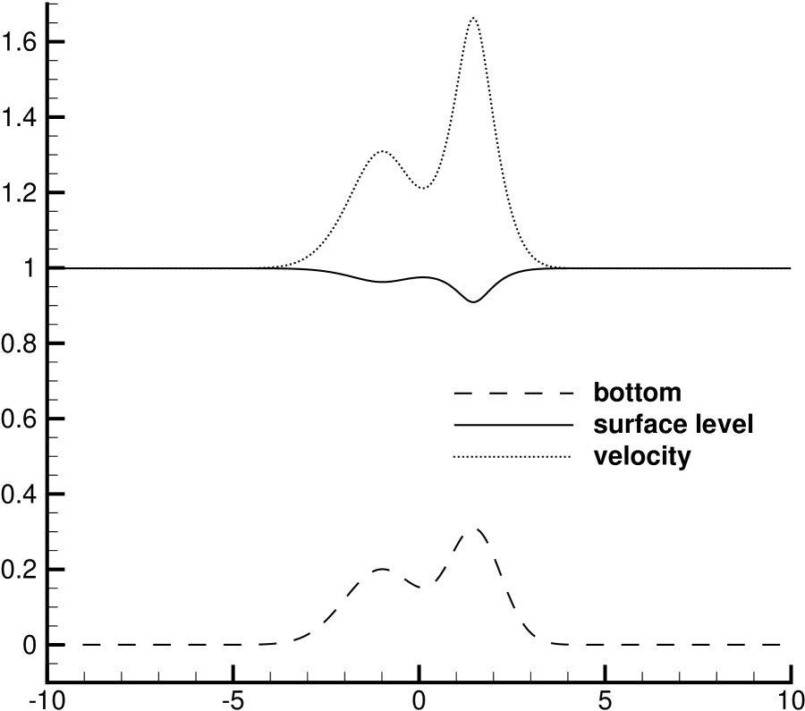
Example 5.4 (Small perturbation of a steady state).

To examine the ability of capturing small perturbation of a steady state, consider two quasi-stationary problems. The first problem is considered in [33, 54]. The bottom topography consists of one hump

b(x)=\begin{cases}0.25(\cos(10\pi(x-1.5))+1),\quad&\text{if}~{}~{}1.4<x<1.6,\\ 0,\quad&\text{otherwise},\end{cases}

and the initial data are

h=\begin{cases}1-b(x)+\epsilon,&\quad\text{if}~{}~{}1.1<x<1.2,\\ 1-b(x),&\quad\text{otherwise},\end{cases}

with zero velocity and zero magnetic field. The second quasi-stationary problem takes into account the magnetic field such that $hB_{1}=1$ . Those problems are solved until $t=0.2$ with the computational domain $[0,2]$ , $g=9.812$ , and $\epsilon=0.2,0.001$ .

The results with zero magnetic field are shown in Figure 5.3, while those with non-zero magnetic field are shown in Figure 5.4. The solutions obtained by using the ES scheme with $N_{x}=200$ are compared to the reference solutions obtained by using the ES scheme with a fine mesh of $N_{x}=3000$ . It can be seen that the structures in the solutions are well captured with no spurious oscillations, and the results with zero magnetic field are well comparable to those in [54].

Example 5.5 (Riemann problem [12]).

The initial data are

(h,v_{1},v_{2},B_{1},B_{2})=\begin{cases}(1,~{}0,~{}0,~{}1,~{}0),&x<0,\\ (2,~{}0,~{}0,~{}0.5,~{}1),&x>0.\end{cases}

The initial discontinuity will be decomposed into two magnetogravity waves and two Alfvén waves propagating away in two directions as the time increases. The problem is solved until $t=0.4$ with $g=1$ .

Figure 5.5 presents the solutions $h,v_{1},v_{2},B_{1},B_{2}$ at $t=0.4$ obtained by the ES schemes with $N_{x}=100$ . One can see that our numerical solutions are in good agreement with the reference solutions, and the discontinuities are well captured without obvious oscillations.

5.2 Two-dimensional case

Example 5.6 (Vortex).

This genuine 2D vortex problem is designed to test the accuracy and the positivity-preserving property of our schemes. With the aid of the SWMHD equations in the polar coordinates given in A, a steady vortex is constructed as follows

	$\displaystyle h^{\prime}=h_{\text{max}}-\left(v_{\text{max}}^{2}-B_{\text{max}}^{2}\right)e^{1-r^{2}}/(2g),$
	$\displaystyle(v_{1}^{\prime},v_{2}^{\prime})=v_{\text{max}}e^{0.5(1-r^{2})}(-y,x),$
	$\displaystyle(B_{1}^{\prime},B_{2}^{\prime})=B_{\text{max}}e^{0.5(1-r^{2})}(-y,x),$

with $v_{\text{max}}=0.2,B_{\text{max}}=0.1,r=\sqrt{x^{2}+y^{2}}$ . Using the Galilean transformation $x^{\prime}=x-t,y^{\prime}=y-t,t^{\prime}=t$ can give a time-dependent exact solution

	$\displaystyle h(x,y,t)=h^{\prime}(x-t,y-t,t),\quad(v_{1},v_{2})(x,y,t)=(1,1)+(v_{1}^{\prime},v_{2}^{\prime})(x-t,y-t,t),$
	$\displaystyle(B_{1},B_{2})(x,y,t)=(B_{1}^{\prime},B_{2}^{\prime})(x-t,y-t,t),$

which describes a vortex moving with a constant speed $(1,1)$ .

The computational domain is $[-8,8]^{2}$ with periodic boundary conditions, $g=1$ , $h_{\text{max}}=1$ , and the output time is $t=16$ so that the vortex travels and returns to the original position after a period. Table 5.3 lists the errors in $h$ and corresponding orders of convergence. The results show that our EC and ES schemes achieve the optimal convergence order. Figure 5.6 plots the contours of $h$ and the magnitude of the magnetic field $|\bm{B}|$ with $40$ equally spaced contour lines. It can be seen that our schemes can preserve the shape of the vortex well after a whole period.

To check the positivity-preserving property, let us do a test with

h_{\text{max}}=10^{-6}+\left(v_{\text{max}}^{2}-B_{\text{max}}^{2}\right)e/(2g),

which implies that the lowest water height is $10^{-6}$ . The errors and orders of convergence obtained by using the ES scheme with or without the positivity-preserving (PP) limiter are listed in Table 5.4. One can see that the ES scheme fails with $N_{x}=N_{y}=20,40$ and without the positivity-preserving limiter, and the positivity-preserving limiter does not destroy the high-order accuracy.

$N_{x}=N_{y}$	EC scheme				ES scheme
$N_{x}=N_{y}$	$\ell^{1}$ error	order	$\ell^{\infty}$ error	order	$\ell^{1}$ error	order	$\ell^{\infty}$ error	order
20	4.079e-05	-	1.787e-02	-	3.756e-05	-	2.446e-02	-
40	7.025e-07	5.86	1.543e-03	3.53	4.082e-06	3.20	1.012e-02	1.27
80	6.401e-09	6.78	3.028e-05	5.67	1.015e-07	5.33	7.531e-04	3.75
160	5.244e-11	6.93	4.994e-07	5.92	1.582e-09	6.00	2.340e-05	5.01
320	4.143e-13	6.98	7.904e-09	5.98	2.453e-11	6.01	7.205e-07	5.02

Table 5.3: Example 5.6: Errors and orders of convergence in

h

t=16

obtained by using the EC and ES schemes,

h_{\text{max}}=1

$N_{x}=N_{y}$	Without PP limiter				With PP limiter
$N_{x}=N_{y}$	$\ell^{1}$ error	order	$\ell^{\infty}$ error	order	$\ell^{1}$ error	order	$\ell^{\infty}$ error	order
20	-	-	-	-	4.007e-05	-	2.680e-02	-
40	-	-	-	-	3.426e-06	3.55	7.087e-03	1.92
80	1.109e-07	-	2.284e-03	-	1.209e-07	4.82	2.657e-03	1.42
160	6.357e-09	4.25	1.000e-03	1.41	5.520e-09	4.45	9.224e-04	1.53
320	3.094e-11	7.68	1.703e-05	5.88	3.089e-11	7.48	1.703e-05	5.76

Table 5.4: Example 5.6: Errors and orders of convergence in

h

t=16

obtained by using the ES schemes,

h_{\text{max}}=10^{-6}+\left(v_{\text{max}}^{2}-B_{\text{max}}^{2}\right)e/(2g)

Example 5.7 (Well-balanced test [33]).

It is used to validate the well-balanced property of our EC and ES schemes. The bottom topography is taken as

b(x,y)=0.8\exp(-5(x-0.9)^{2}-50(y-0.5)^{2}),

(5.3)

b(x,y)=0.5\chi_{[0.5,1.5]\times[0.25,0.75]}.

(5.4)

The computational domain is $[0,2]\times[0,1]$ , $g=1$ , and the initial data are $h(x,y)=1-b(x,y)$ with zero velocity and magnetic field.

The problem is solved until $t=1$ with $N_{x}=N_{y}=40$ . The errors in $h,v_{1},v_{2}$ are listed in Table 5.5. Similar to Example 5.2, one can see that the well-balanced property of the 2D schemes has been verified in the sense that the errors are at the level of round-off errors for the double precision.

		EC scheme		ES scheme
		$\ell^{1}$ error	$\ell^{\infty}$ error	$\ell^{1}$ error	$\ell^{\infty}$ error
(5.3)	$h$	4.943e-15	3.886e-14	2.293e-15	1.077e-14
	$v_{1}$	5.091e-15	4.091e-14	2.577e-15	1.010e-14
	$v_{2}$	3.766e-15	3.168e-14	1.887e-15	9.742e-15
(5.4)	$h$	8.437e-16	5.329e-15	8.102e-16	4.663e-15
	$v_{1}$	5.720e-16	4.585e-15	5.731e-16	3.792e-15
	$v_{2}$	1.385e-15	7.659e-15	1.367e-15	6.306e-15

Table 5.5: Example 5.7: Errors in

h,v_{1},v_{2}

t=1

for the bottom topography (5.3) and (5.4).

Example 5.8 (Small perturbation of a steady state (without magnetic field) [33]).

This problem is used to check the capability of the ES schemes for the perturbation of the steady state. The computational domain and the bottom topography are the same as the last test, and the initial data are

h=\begin{cases}1.01-b(x),&\text{if}~{}~{}0.05<x<0.15,\\ 1-b(x),&\text{otherwise},\end{cases}

with zero velocity and magnetic field. Outflow boundary conditions are used and the problem is solved until $t=0.6$ with $g=9.812$ .

Figure 5.7 shows the contours of the surface level $h+b$ (40 equally spaced contour lines) at $t=0.12,0.24,0.36,0.48,0.6$ obtained by using the ES scheme with $N_{x}=600,N_{y}=300$ , which describe a right-going disturbance as it propagates past the hump. It can be seen that the complex small features are well captured without any spurious oscillations, and the results are comparable to those in [54].

Example 5.9 (Orszag-Tang like problem [56]).

It is similar to the Orszag-Tang problem for the ideal MHD equations [38]. The computational domain is $[0,2\pi]^{2}$ with periodic boundary conditions and $g=1$ . The initial data are

\displaystyle(h,v_{1},v_{2},B_{1},B_{2})=(25/9,-\sin y,\sin x,-\sin y,\sin 2x).

The solution of this problem is smooth initially, but the complicated pattern will arise as the time increases and it has the turbulence behavior. Figure 5.8 presents the results obtained by using the ES scheme with $N_{x}=N_{y}=200$ at $t=1$ and $2$ . The solutions are in good agreement with those in [56]. The left plot in Figure 5.10 shows the time evolution of the discrete total entropy $\sum_{i,j}\eta(\bm{U}_{i,j})\Delta x\Delta y$ with three spatial resolutions $N_{x}=N_{y}=100$ , 200 and 400. The total entropy is conserved when the solutions are smooth during an initial period, but it decays when discontinuities arise.

Example 5.10 (Rotor like problem [30]).

It is an extension of the classical ideal MHD rotor test problem [30]. The computational domain is $[-1,1]^{2}$ with outflow conditions with $g=1$ . Initially $hB_{1}=1$ and $hB_{2}=0$ , and there is a disk of radius $r_{0}=0.1$ centered at $(0,0)$ , where fluid with large $h$ is rotating in the anti-clockwise direction. The ambient fluid is homogeneous for $r>r_{0}$ , where $r=\sqrt{x^{2}+y^{2}}$ . Specifically, the initial data are

\displaystyle(h,v_{1},v_{2})=\begin{cases}(10,-y,~{}x),&r<r_{0},\\ (1,~{}0,~{}0),&r>r_{0}.\\ \end{cases}

This problem is solved until $t=0.2$ .

Figure 5.9 shows the height $h$ , the velocity $\bm{v}$ , and the magnetic field $\bm{B}$ obtained by using the ES scheme with $N_{x}=N_{y}=400$ . The ES scheme gets the high resolution results without obvious spurious oscillations comparable to those in [30]. The right plot of Figure 5.10 displays the time evolution of the discrete total entropy with three spatial resolutions $N_{x}=N_{y}=100$ , 200 and 400. The results show that the total entropy decays as expected, and the fully discrete scheme is also ES.

6 Conclusion

The paper proposed the high-order accurate entropy stable (ES) finite difference schemes for the one- and two-dimensional shallow water magnetohydrodynamic (SWMHD) equations with non-flat bottom topography. The Janhunen source term was added to the conservative SWMHD equations. For the modified SWMHD equations, the second-order accurate well-balanced semi-discrete entropy conservative (EC) finite difference scheme was first constructed, in the sense that it satisfied the semi-discrete entropy identity for the given entropy pair (the total energy served as the mathematical entropy) and preserved the steady state of lake at rest (with zero magnetic field). The key was to match both discretizations for the fluxes and the source term related to the non-flat river bed bottom and the Janhunen source term, and to find the affordable EC fluxes of the second-order EC schemes. Next, the high-order accurate well-balanced EC schemes were obtained by using the second-order accurate EC schemes as building block. In view of that the EC schemes might become oscillatory near the discontinuities, the appropriate dissipation terms were added to the EC fluxes to develop the semi-discrete well-balanced ES schemes satisfying the semi-discrete entropy inequality. The WENO reconstruction of the scaled entropy variables and the high-order explicit Runge-Kutta time discretization were implemented to obtain the fully-discrete high-order schemes. The ES and positivity-preserving properties of the Lax-Friedrichs scheme were also proved without the assumption that the 1D exact Riemann solution of $x$ -split system was ES, and then the high-order positivity-preserving ES schemes were developed by using the positivity-preserving flux limiter. Extensive numerical tests showed that our schemes could achieve the designed accuracy, were well-balanced or positivity-preserving, and could well capture the discontinuities.

Appendix A SWMHD in polar coordinates

In the polar coordinate system $(r,\theta)$ , the modified SWMHD equations (2.4) without the bottom topography become

		$\displaystyle\dfrac{\partial{h}}{\partial{t}}+\nabla\cdot(h\bm{v})=0,$		(A.1)
		$\displaystyle\dfrac{\partial{(hv_{r})}}{\partial{t}}+\nabla\cdot(hv_{r}\bm{v}-hB_{r}\bm{B})+\dfrac{\partial{(gh^{2}/2)}}{\partial{r}}=\dfrac{h(v_{\theta}^{2}-B_{\theta}^{2})}{r},$
		$\displaystyle\dfrac{\partial{(hv_{\theta})}}{\partial{t}}+\nabla^{r}\cdot(hv_{\theta}\bm{v}-hB_{\theta}\bm{B})+\dfrac{\partial{(gh^{2}/2)}}{\partial{\theta}}=0,$
		$\displaystyle\dfrac{\partial{(hB_{r})}}{\partial{t}}+\dfrac{1}{r}\dfrac{\partial{(hv_{\theta}B_{r}-hv_{r}B_{\theta})}}{\partial{\theta}}=-B_{r}\nabla\cdot(h\bm{B}),$
		$\displaystyle\dfrac{\partial{(hB_{\theta})}}{\partial{t}}-\dfrac{\partial{(hv_{\theta}B_{r}-hv_{r}B_{\theta})}}{\partial{r}}=-B_{\theta}\nabla\cdot(h\bm{B}),$

where

\displaystyle\nabla\cdot\bm{F}=\dfrac{1}{r}\dfrac{\partial{(rF_{r})}}{\partial{r}}+\dfrac{1}{r}\dfrac{\partial{F_{\theta}}}{\partial{\theta}},\quad\nabla^{r}\cdot\bm{F}=\dfrac{1}{r^{2}}\dfrac{\partial{(r^{2}F_{r})}}{\partial{r}}+\dfrac{1}{r}\dfrac{\partial{F_{\theta}}}{\partial{\theta}},

(A.2)

and $F_{r},F_{\theta}$ are the radius and azimuth components of the vector $\bm{F}$ , respectively.

Acknowledgments

The authors would like to thank the discussion of Dr. Kailiang Wu at The Ohio State University and Mr. Caiyou Yuan at Peking University. The work was partially supported by the Special Project on High-performance Computing under the National Key R&D Program (No. 2016YFB0200603), Science Challenge Project (No. TZ2016002), the National Natural Science Foundation of China (Nos. 91630310 & 11421101), and High-performance Computing Platform of Peking University.

References

[1] S. Ahmed and S. Zia, The higher-order CESE method for two-dimensional shallow water magnetohydrodynamics equations, Eur. J. Pure Appl. Math., 12 (2019), pp. 1464–1482.
[2] D. S. Balsara, Divergence-free reconstruction of magnetic fields and WENO schemes for magnetohydrodynamics, J. Comput. Phys., 228 (2009), pp. 5040–5056.
[3] T. J. Barth, Numerical methods for gasdynamic systems on unstructured meshes, in An Introduction to Recent Developments in Theory and Numerics for Conservation Laws, D. Kroner, M. Ohlberger, and C. Rohde, eds., Springer, 1999, pp. 195–285.
[4] A. Bermudez and M. E. Vazquez, Upwind methods for hyperbolic conservation laws with source terms, Comput. & Fluids, 23 (1994), pp. 1049–1071.
[5] B. Biswas and R. K. Dubey, Low dissipative entropy stable schemes using third order WENO and TVD reconstructions, Adv. Comput. Math., 44 (2018), pp. 1153–1181.
[6] R. Borges, M. Carmona, B. Costa, and W. S. Don, An improved weighted essentially non-oscillatory scheme for hyperbolic conservation laws, J. Comput. Phys., 227 (2008), pp. 3191–3211.
[7] F. Bouchut, C. Bourdarias, and B. Perthame, A muscl method satisfying all the numerical entropy inequalities, Math. Comp., 65 (1996), pp. 1439–1461.
[8] J. U. Brackbill and D. C. Barnes, The effect of nonzero $\nabla\cdot{\bf B}$ on the numerical solution of the magnetohydrodynamic equations, J. Comput. Phys., 35 (1980), pp. 426–430.
[9] P. Chandrashekar and C. Klingenberg, Entropy stable finite volume scheme for ideal compressible MHD on 2D Cartesian meshes, SIAM J. Numer. Anal., 54 (2016), pp. 1313–1340.
[10] T. Chen and C.-w. Shu, Entropy stable high order discontinuous Galerkin methods with suitable quadrature rules for hyperbolic conservation, J. Comput. Phys., 345 (2017), pp. 427–461.
[11] M. G. Crandall and A. Majda, Monotone difference approximations for scalar conservation laws, Math. Comp., 34 (1980), pp. 1–21.
[12] H. De Sterck, Hyperbolic theory of the “shallow water” magnetohydrodynamics equations, Phys. Plasmas, 8 (2001), pp. 3293–3304.
[13] A. Dedner, F. Kemm, D. Kröner, C. D. Munz, T. Schnitzer, and M. Wesenberg, Hyperbolic divergence cleaning for the MHD equations, J. Comput. Phys., 175 (2002), pp. 645–673.
[14] D. Derigs, A. R. Winters, G. J. Gassner, S. Walch, and M. Bohm, Ideal GLM-MHD: About the entropy consistent nine-wave magnetic field divergence diminishing ideal magnetohydrodynamics equations, J. Comput. Phys., 364 (2018), pp. 420–467.
[15] J. Duan and H. Tang, High-order accurate entropy stable nodal discontinuous galerkin schemes for the ideal special relativistic magnetohydrodynamics, arXiv:1911.03825, (2019).
[16] , High-order accurate entropy stable finite difference schemes for one- and two-dimensional special relativistic hydrodynamics, Adv. Appl. Math. Mech., 12 (2020), pp. 1–29.
[17] C. R. Evans and J. F. Hawley, Simulation of magnetohydrodynamic flows-a constrained transport method, Astrophys. J., 332 (1988), pp. 659–677.
[18] T. C. Fisher and M. H. Carpenter, High-order entropy stable finite difference schemes for nonlinear conservation laws: Finite domains, J. Comput. Phys., 252 (2013), pp. 518–557.
[19] U. S. Fjordholm, S. Mishra, and E. Tadmor, Well-balanced and energy stable schemes for the shallow water equations with discontinuous topography, J. Comput. Phys., 230 (2011), pp. 5587–5609.
[20] , Arbitrarily high-order accurate entropy stable essentially non-oscillatory schemes for systems of conservation laws, SIAM J. Numer. Anal., 50 (2012), pp. 544–573.
[21] , ENO reconstruction and ENO interpolation are stable, Found. Comput. Math., 13 (2013), pp. 139–159.
[22] G. J. Gassner, A. R. Winters, and D. A. Kopriva, A well balanced and entropy conservative discontinuous Galerkin spectral element method for the shallow water equations, Appl. Math. Comput., 272 (2016), pp. 291–308.
[23] P. A. Gilman, Magnetohydrodynamic “shallow water” equations for the solar tachocline, Astrophys. J., 544 (2000), pp. L79–L82.
[24] A. Harten, On the symmetric form of systems of conservation laws with entropy, J. Comput. Phys., 49 (1983), pp. 151–164.
[25] A. Hiltebrand and S. Mishra, Entropy stable shock capturing space – time discontinuous Galerkin schemes for systems of conservation laws, Numer. Math., 126 (2014), pp. 103–151.
[26] X. Y. Hu, N. A. Adams, and C. W. Shu, Positivity-preserving method for high-order conservative schemes solving compressible Euler equations, J. Comput. Phys., 242 (2013), pp. 169–180.
[27] T. J. Hughes, L. Franca, and M. Mallet, A new finite element formulation for computational fluid dynamics: I. symmetric forms of the compressible euler and navier-stokes equations and the second law of thermodynamics, Comput. Methods Appl. Mech. Engrg., 54 (1986), pp. 223–234.
[28] P. Janhunen, A positive conservative method for magnetohydrodynamics based on HLL and Roe methods, J. Comput. Phys., 160 (2000), pp. 649–661.
[29] F. Kemm, Roe-type schemes for shallow water magnetohydrodynamics with hyperbolic divergence cleaning, Appl. Math. Comput., 272 (2016), pp. 385–402.
[30] T. Kröger and M. Lukáčová-Medvid’ová, An evolution Galerkin scheme for the shallow water magnetohydrodynamic equations in two space dimensions, J. Comput. Phys., 206 (2005), pp. 122–149.
[31] Y. Kuang, K. Wu, and H. Tang, Runge-Kutta discontinuous local evolution Galerkin methods for the shallow water equations on the cubed-sphere grid, Numer. Math. Theor. Meth. Appl., 10 (2017), pp. 373–419.
[32] P. G. Lefloch, J. M. Mercier, and C. Rohde, Fully discrete entropy conservative schemes of arbitraty order, SIAM J. Numer. Anal., 40 (2002), pp. 1968–1992.
[33] R. J. LeVeque, Balancing source terms and flux gradients in high-resolution Godunov methods: the quasi-steady wave-propagation algorithm, J. Comput. Phys., 146 (1998), pp. 346–365.
[34] F. Li and C. W. Shu, Locally divergence-free discontinuous Galerkin methods for MHD equations, J. Sci. Comput., 22 (2005), pp. 413–442.
[35] F. Li and L. Xu, Arbitrary order exactly divergence-free central discontinuous Galerkin methods for ideal MHD equations, J. Comput. Phys., 231 (2011), pp. 2655–2675.
[36] P. Londrillo and L. Del Zanna, On the divergence-free condition in Godunov-type schemes for ideal magnetohydrodynamics: the upwind constrained transport method, J. Comput. Phys., 195 (2004), pp. 17–48.
[37] S. Noelle, Y. Xing, and C.-W. Shu, High-order well-balanced finite volume WENO schemes for shallow water equation with moving water, J. Comput. Phys., 226 (2007), pp. 29–58.
[38] S. A. Orszag and C. M. Tang, Small-scale structure of two-dimensional magnetohydrodynamic turbulence, J. Fluid Mech., 90 (1979), pp. 129–143.
[39] S. Osher, Riemann solvers, the entropy condition, and difference, SIAM J. Numer. Anal., 21 (1984), pp. 217–235.
[40] S. Osher and E. Tadmor, On the convergence of difference approximations to scalar conservation laws, Math. Comp., 50 (1988), pp. 19–51.
[41] K. G. Powell, An approximate riemann solver for magnetohydrodynamics (that works in more than one dimension), ICASE 94-24, (1994).
[42] S. Qamar and G. Warnecke, Application of space-time CE/SE method to shallow water magnetohydrodynamic equations, J. Comput. Appl. Math., 196 (2006), pp. 132–149.
[43] J. A. Rossmanith, A constrained transport method for the shallow water mhd equations, in Hyperbolic Problems: Theory, Numerics, Applications, T. Hou and E. Tadmor, eds., Springer, 2003, pp. 851–860.
[44] J. A. Rossmanith, An unstaggered, high-resolution constrained transport method for magnetohydrodynamic flows, SIAM J. Sci. Comput., 28 (2006), pp. 1766–1797.
[45] E. Tadmor, The numerical viscosity of entropy stable schemes for systems of conservation laws. I, Math. Comput., 49 (1987), pp. 91–103.
[46] , Entropy stability theory for difference approximations of nonlinear conservation laws and related time-dependent problems, Acta Numer., 12 (2003), pp. 451–512.
[47] H. Tang, Solution of the shallow-water equations using an adaptive moving mesh method, Internat. J. Numer. Methods Fluids, 44 (2004), pp. 789–810.
[48] H. Tang, T. Tang, and K. Xu, A gas-kinetic scheme for shallow-water equations with source terms, Z. Angew. Math. Phys., 55 (2004), pp. 365–382.
[49] A. R. Winters and G. J. Gassner, Affordable, entropy conserving and entropy stable flux functions for the ideal MHD equations, J. Comput. Phys., 304 (2016), pp. 72–108.
[50] , An entropy stable finite volume scheme for the equations of shallow water magnetohydrodynamics, J. Sci. Comput., 67 (2016), pp. 514–539.
[51] K. Wu and C.-W. Shu, Entropy symmetrization and high-order accurate entropy stable numerical schemes for relativistic MHD equations, arXiv:1907.07467, (2019).
[52] K. Wu and H. Tang, A Newton multigrid method for steady-state shallow water equations with topography and dry areas, Appl. Math. Mech., 37 (2016), pp. 1441–1466.
[53] Y. Xing, Numerical methods for the nonlinear shallow water equations, vol. 18, Elsevier, 2017, ch. Handbook of Numerical Analysis, pp. 361–384.
[54] Y. Xing and C. W. Shu, High order finite difference WENO schemes with the exact conservation property for the shallow water equations, J. Comput. Phys., 208 (2005), pp. 206–227.
[55] K. Xu, A well-balanced gas-kinetic scheme for the shallow-water equations with source terms, J. Comput. Phys., 178 (2002), pp. 533–562.
[56] S. Zia, M. Ahmed, and S. Qamar, Numerical solution of shallow water magnetohydrodynamic equations with non-flat bottom topography, Int. J. Comut. Fluid Dyn., 28 (2014), pp. 56–75.