\setcopyright

ifaamas \acmConference[AAMAS ’24]Proc. of the 23rd International Conference on Autonomous Agents and Multiagent Systems (AAMAS 2024)May 6 – 10, 2024 Auckland, New ZealandN. Alechina, V. Dignum, M. Dastani, J.S. Sichman (eds.) \copyrightyear2024 \acmYear2024 \acmDOI \acmPrice \acmISBN \acmSubmissionID427 \affiliation \institutionCornell University \cityIthaca \stateNY \countryUSA \affiliation \institutionCornell University \cityIthaca \stateNY \countryUSA

High-Level, Collaborative Task Planning Grammar and Execution for Heterogeneous Agents

Amy Fang [email protected] and Hadas Kress-Gazit [email protected]

Abstract.

We propose a new multi-agent task grammar to encode collaborative tasks for a team of heterogeneous agents that can have overlapping capabilities. The grammar allows users to specify the relationship between agents and parts of the task without providing explicit assignments or constraints on the number of agents required. We develop a method to automatically find a team of agents and synthesize correct-by-construction control with synchronization policies to satisfy the task. We demonstrate the scalability of our approach through simulation and compare our method to existing task grammars that encode multi-agent tasks.

Key words and phrases:

Formal methods, multiagent coordination, task planning, robotics

1. Introduction

Agents working together to achieve common goals have a variety of applications, such as warehouse automation or disaster response. Multi-agent tasks have been defined in different ways in the scheduling and planning literature. For example, in multi-agent task allocation Jia and Meng (2013); Gerkey and Matarić (2004); Korsah et al. (2013) and coalition formation Xu et al. (2015); Li et al. (2009), each task is a single goal with an associated utility. Individual agents or agent teams then automatically assign themselves to a task based on some optimization metric. Swarm approaches Schmickl et al. (2006); Wang and Rubenstein (2020) consider emergent behavior of an agent collective as the task, for example, aggregation or shape formation.

Recently, formal methods, such as temporal logics for task specifications and correct-by-construction synthesis, have been used to solve different types of multi-agent planning tasks Ulusoy et al. (2012); Schillinger et al. (2018); Chen et al. (2021). Tasks written in temporal logic, such as Linear Temporal Logic (LTL), allow users to capture complex tasks with temporal constraints. Existing work has extended LTL Luo and Zavlanos (2022); Sahin et al. (2017) and Signal Temporal Logic Leahy et al. (2022) to encode tasks that require multiple agents.

In this paper, we consider tasks that a team of heterogeneous agents are required to collaboratively satisfy. For instance, consider a precision agriculture scenario in which a farm contains agents with different on-board sensors to monitor crop health. The user may want to take a moisture measurement in one region, and then take a soil sample of a different region. Depending on the agents’ sensors and sensing range, the agents may decide to collaborate to satisfy the task. For example, one agent may perform the entire task on its own if it has both a moisture sensor and an arm mechanism to pick up a soil sample and can move between the two regions. However, another possible solution is for two agents to team up so that one takes a moisture measurement and the other picks up the soil. Existing task grammars Luo and Zavlanos (2022); Sahin et al. (2017); Leahy et al. (2022) capture tasks such as the above by providing explicit constraints on the types or number of agents for each part of the task, i.e. the task must explicitly encode whether it should be one agent, two agents, or either of these options. In this paper, we create a task grammar and associated control synthesis that removes the need to a priori decide on the number of agents necessary to accomplish a task, allowing users to focus solely on the actions required to achieve the task (e.g. “take a moisture measurement and then pick up a soil sample, irrespective of which or how many agents perform which actions”).

Our task grammar has several unique aspects. First, this grammar enables the interleaving of agent actions, alleviating the need for explicit task decomposition in order to assign agents to parts of the task. Second, rather than providing explicit constraints on the types or number of agents for each part of the task, the task encodes, using the concept of bindings (inspired by Luo and Zavlanos (2022)), the overall relationship between agent assignments and team behavior; we can require certain parts of the task to be satisfied by the same agent without assigning the exact agent or type of agent a priori. Lastly, the grammar allows users to make the distinction between the requirements “for all agents” and “at least one agent”. Given these types of tasks, agents autonomously determine, based on their capabilities, which parts of the task they can and should do for the team to satisfy the task.

Tasks may require collaboration between different agents. Similar to Kloetzer and Belta (2010); Tumova and Dimarogonas (2016); Chen et al. (2011), to ensure the actions are performed in the correct order, our framework takes the corresponding synchronization constraints into account while synthesizing agent behavior; agents must wait to execute the actions together. In our approach, execution of the synchronous behavior for each agent is decentralized; agents carry out their plan and communicate with one another when synchronization is necessary.

Depending on the task and the available agents, there might be different teams (i.e., subsets of the agent set) that can carry out the task; our algorithm for assigning a team and synthesizing behavior for the agents finds the largest team of agents that satisfies the task. This means that the team may have redundancies, i.e. agents can be removed while still ensuring the overall task is satisfied. This is beneficial both for robustness and optimality; the user can choose a subset of the team (provided that all the required bindings are still assigned) to optimize different metrics, such as cost or overall number of agents.

Related work: One way to encode tasks is to first decompose them into independent sub-tasks and then allocate them to the agents. For example, Schillinger et al. (2018); Faruq et al. (2018) address finite-horizon tasks for multi-agent teams. The authors first automatically decompose a global automaton representing the task into independent sub-tasks. To synthesize control policies, the authors build product automata for each heterogeneous agent. Each automaton is then sequentially linked using switch transitions to reduce state-space explosion in synthesizing parallel plans. In our prior work Fang and Kress-Gazit (2022), we address infinite-horizon tasks that have already been decomposed into sub-tasks. Given a new task, we proposed a decentralized framework for agents to automatically update their behavior based on a new task and their existing tasks, allowing agents to interleave the tasks.

The works discussed above make the critical assumption that tasks are independent, i.e. agents do not collaborate with one another. One approach to including collaborative actions is to explicitly encode the agent assignments in the tasks. To synthesize agent control for these types of tasks, in Tumova and Dimarogonas (2016), the authors construct a reduced product automaton in which the agents only synchronize when cooperative actions are required. The work in Kantaros and Zavlanos (2020) proposes a sampling-based method that approximates the product automaton of the team by building trees incrementally while maintaining probabilistic completeness. In this paper, we consider the more general setting in which agents may need to collaborate with each other, but are not given explicit task assignments a priori.

Rather than providing predetermined task assignments, another approach for defining collaborative tasks is to capture information about the number and type of agents needed for parts of the specification. For example, Sahin et al. (2017) imposes constraints on the number of agents necessary in regions using counting LTL. Leahy et al. (2022) uses Capability Temporal Logic to encode both the number and capabilities necessary in certain abstracted locations in the environment and then formulates the problem as a MILP to find an optimal teaming strategy. The authors of Luo and Zavlanos (2022) introduce the concept of induced propositions, where each atomic proposition not only encodes information about the number, type of agents, and target regions, but also has a connector that binds the truth of certain atomic propositions together. To synthesize behavior for the agents, they propose a hierarchical approach that first constructs the automaton representing the task and then decomposes the task into possible sub-tasks. The temporal order of these sub-tasks is captured using partially ordered sets and are used in the task allocation problem, which is formulated as a MILP.

Inspired by Luo and Zavlanos (2022) and the concept of induced propositions, we create a task grammar that includes information about how the atomic propositions are related to one another, which represents the overall relationship between agents and task requirements. Unlike Luo and Zavlanos (2022), which considers navigation tasks in which the same set of agents of a certain type may need to visit different regions, we generalize these tasks to any type of abstract action an agent may be able to perform. In addition, a key assumption we relax is that we do not require each agent to be only categorized as one type. As a result, agents can have overlapping capabilities. To our knowledge, no other grammars have been proposed for these generalized types of multi-agent collaborative tasks.

Contributions: We propose a task description and control synthesis framework for heterogeneous agents to satisfy collaborative tasks. Specifically, we present a new, LTL-based task grammar for the formulation of collaborative tasks, and provide a framework to form a team of agents and synthesize control and synchronization policies to guarantee the team satisfies the task. We demonstrate our approach in simulated precision agriculture scenarios.

2. Preliminaries

2.1. Linear Temporal Logic

LTL formulas are defined over a set of atomic propositions $AP$ , where $\pi\in AP$ are Boolean variables Emerson (1990). We abstract agent actions as atomic propositions. For example, $UV$ captures an agent taking UV measurement.

Syntax: An LTL formula is defined as:

\varphi::=\pi\ |\ \neg\varphi\ |\ \varphi\vee\varphi\ |\ \bigcirc\varphi\ |\ \varphi\ \mathcal{U}\ \varphi

where $\neg$ (“not”) and $\vee$ (“or”) are Boolean operators, and $\bigcirc$ (“next”) and $\mathcal{U}$ (“until”) are temporal operators. From these operators, we can define: conjunction $\varphi\wedge\varphi$ , implication $\varphi\Rightarrow\varphi$ , eventually $\Diamond\varphi=\text{True}\ \mathcal{U}\ \varphi$ , and always $\Box\varphi=\neg\Diamond\neg\varphi$ .

Semantics: The semantics of an LTL formula $\varphi$ are defined over an infinite trace $\sigma=\sigma(0)\sigma(1)\sigma(2)...$ , where $\sigma(i)$ is the set of true $AP$ at position $i$ . We denote that $\sigma$ satisfies LTL formula $\varphi$ as $\sigma\models\varphi$ .

Intuitively, $\Diamond\varphi$ is satisfied if there exists a $\sigma(i)$ in which $\varphi$ is true. $\Box\varphi$ is satisfied if $\varphi$ is true at every position in $\sigma$ . To satisfy $\varphi_{1}\ \mathcal{U}\ \varphi_{2}$ , $\varphi_{1}$ must remain true until $\varphi_{2}$ becomes true. See Emerson (1990) for the full semantics.

2.2. Büchi Automata

An LTL formula $\varphi$ can be translated into a Nondeterministic Büchi Automaton that accepts infinite traces if and only if they satisfy $\varphi$ . A Büchi automaton is a tuple $\mathcal{B}=(Z,z_{0},\Sigma_{\mathcal{B}},\delta_{\mathcal{B}},F)$ , where $Z$ is the set of states, $z_{0}\in Z$ is the initial state, $\Sigma_{\mathcal{B}}$ is the input alphabet, $\delta_{\mathcal{B}}:Z\times\Sigma_{\mathcal{B}}\times Z$ is the transition relation, and $F\subseteq Z$ is a set of accepting states. An infinite run of $\mathcal{B}$ over a word $w=w_{1}w_{2}w_{3}...$ , $w_{i}\in\Sigma_{\mathcal{B}}$ is an infinite sequence of states $z=z_{0}z_{1}z_{2}...$ such that $(z_{i-1},w_{i},z_{i})\in\delta_{\mathcal{B}}$ . A run is accepting if and only if Inf( $z$ ) $\cap\ F\neq\emptyset$ , where Inf( $z$ ) is the set of states that appear in $z$ infinitely often Baier and Katoen (2008).

2.3. Agent Model

Following Fang and Kress-Gazit (2022), we create an abstract model for each agent based on its set of capabilities. A capability is a weighted transition system $\mathcal{\lambda}=(S,s_{0},AP,\Delta,L,W)$ , where $S$ is a finite set of states, $s_{0}\in S$ is the initial state, $AP$ is the set of atomic propositions, $\Delta\subseteq S\times S$ is a transition relation where for all $s\in S$ , $\exists s^{\prime}\in S$ such that $(s,s^{\prime})\in\Delta$ , $L:S\rightarrow 2^{AP}$ is the labeling function such that $L(s)$ is the set of propositions that are true in state $s$ , and $W:\Delta\rightarrow\mathbb{R}_{\geq 0}$ is the cost function assigning a weight to each transition. Since we are considering a group of heterogeneous agents, agent $j$ has its own set of $k$ capabilities $\Lambda_{j}=\{\lambda_{1},...,\lambda_{k}\}$ .

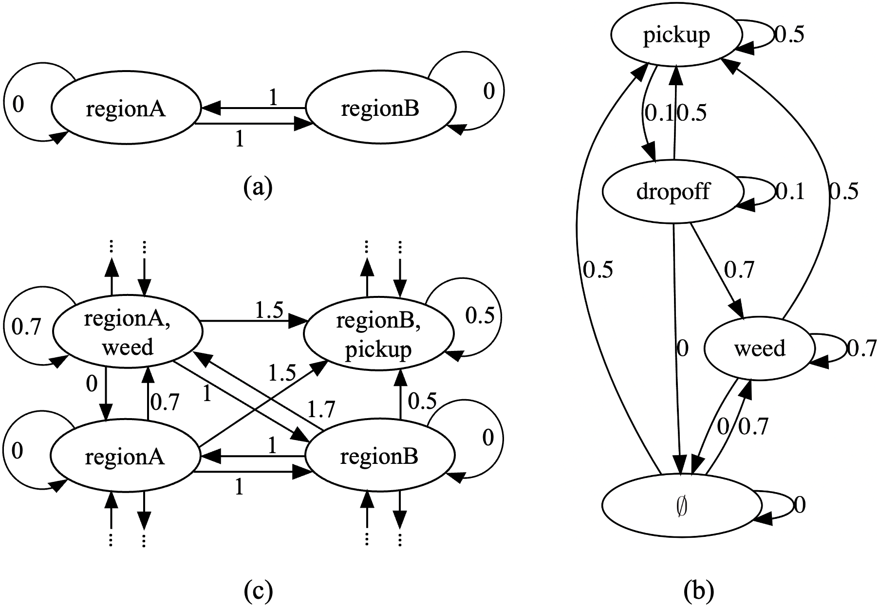
An agent model $A_{j}$ is the product of its capabilities: $A_{j}=\lambda_{1}\times...\times\lambda_{k}$ such that $A_{j}=(S,s_{0},AP_{j},\gamma,L,W)$ , where $S=S_{1}\times...\times S_{k}$ is the set of states, $s_{0}\in S$ is the initial state, $AP_{j}=\bigcup_{i=1}^{k}AP_{i}$ is the set of propositions, $\gamma\subseteq S\times S$ is the transition relation such that $(s,s^{\prime})\in\gamma$ , where $s=(s_{1},...,s_{k}),s^{\prime}=(s^{\prime}_{1},...,s^{\prime}_{k})$ , if and only if for all $i=\{1,...,k\},(s_{i},s^{\prime}_{i})\in\Delta_{i}$ , $L:S\rightarrow 2^{AP_{j}}$ is the labeling function where $L(s)=\bigcup_{i=1}^{k}L_{i}(s_{i})$ , and $W:\gamma\rightarrow\mathbb{R}_{\geq 0}$ is the cost function that combines the costs of the capabilities. Fig. 1c depicts a snippet of an agent model where we treat the cost as additive. Fig. 1a represents the agent’s sensing area $\lambda_{area}$ ; the agent can orient its sensors to take measurements in different regions of a partitioned workspace (in this case, regions A and B). Fig. 1b represents the agent’s robot manipulator, which can pick up and drop off soil samples, as well as pull weeds.

Refer to caption — Figure 1. Agent partial model: (a) $\lambda_{\mathit{area}}$ (b) $\lambda_{\mathit{arm}}$ (c) $A_{green}$

3. Task Grammar - LTL^ψ

We define the task grammar LTL^ψ that includes atomic propositions that abstract agent action, logical and temporal operators, as in LTL, and bindings that connect actions to specific agents; any action labeled with the same binding must be satisfied by the same agent(s) (the actual value of the binding is not important). We define a task recursively over LTL and binding formulas.

$\displaystyle\psi$	$\displaystyle:=\rho\>\|\>\psi_{1}\vee\psi_{2}\>\|\>\psi_{1}\wedge\psi_{2}$	(1)
$\displaystyle\varphi$	$\displaystyle:=\pi\ \|\ \neg\varphi\ \|\ \varphi\vee\varphi\ \|\bigcirc\varphi\ \|\ \varphi\ \mathcal{U}\ \varphi$	(2)
$\displaystyle\varphi^{\psi}\!$	$\displaystyle:=\varphi^{\psi}\!\>\|\>\neg(\varphi^{\psi})\>\|\>\!\varphi_{1}^{\psi_{1}}\!\!\wedge\!\varphi_{2}^{\psi_{2}}\|\ \!\varphi_{1}^{\psi_{1}}\!\!\vee\!\varphi_{2}^{\psi_{2}}\!\>\|\>\!\!\bigcirc\!\varphi^{\psi}\!\>\|\>\varphi_{1}^{\psi_{1}}\mathcal{U}\varphi_{2}^{\psi_{2}}\!\>\|\>\Box\varphi^{\psi}$	(3)

where $\psi$ , the binding formula, is a Boolean formula excluding negation over $\rho\in AP_{\psi}$ , and $\varphi$ is an LTL formula. An LTL^ψ formula consists of conjunction, disjunction, and temporal operators; we define eventually as $\Diamond\varphi^{\psi}=\text{True}\ \mathcal{U}\ \varphi^{\psi}$ . An example of an LTL^ψ formula is shown in Eq. 4.

Semantics: The semantics of an LTL^ψ formula $\varphi^{\psi}$ are defined over $\sigma$ and $R$ ; $\sigma=\sigma_{1}\sigma_{2}...\sigma_{n}$ is the team trace where $\sigma_{j}$ is agent $j$ ’s trace, and $\forall i,\sigma(i)=\sigma_{1}(i)\sigma_{2}(i)...\sigma_{n}(i)$ . $R=\{r_{1},r_{2},...,r_{n}\}$ is the set of binding assignments, where $r_{j}\in R$ is the set of $AP_{\psi}$ that are assigned to agent $j$ . Once a team is established, $R$ is constant, i.e. an agent’s binding assignment does not change throughout the task execution. For example, $r_{1}=\{2,3\},r_{2}=\{1\}$ denotes that agent 1 is assigned bindings 2 and 3, and agent 2 is assigned binding 1.

Given $n$ agents and a set of binding propositions $AP_{\psi}$ , we define the function $\zeta:\psi\rightarrow 2^{2^{AP_{\psi}}}$ such that $\zeta(\psi)$ is the set of all possible combinations of $\rho$ that satisfy $\psi$ . For example, $\zeta\bigl{(}(1\vee 2)\wedge 3\bigr{)}=\{\{1,3\},\{2,3\},\{1,2,3\}\}$ .

The semantics of LTL^ψare:

•

$(\sigma(i),R)\!\models\varphi^{\psi}$ iff $\exists K\in\zeta(\psi)$ s.t. ( $K\subseteq\bigcup\limits_{p=1}^{n}r_{p}$ ) and ( $\forall j$ s.t. $K\cap r_{j}\neq\emptyset$ , $\sigma_{j}(i)\models\varphi$ )
•

$(\sigma(i),R)\!\models(\neg\varphi)^{\psi}$ iff $\exists K\in\zeta(\psi)$ s.t. ( $K\subseteq\bigcup\limits_{p=1}^{n}r_{p}$ ) and ( $\forall j$ s.t. $K\cap r_{j}\neq\emptyset$ , $\sigma_{j}(i)\not\models\varphi$ )
•

$(\sigma(i),R)\!\models\neg(\varphi^{\psi})$ iff $\exists K\in\zeta(\psi)$ s.t. ( $K\subseteq\bigcup\limits_{p=1}^{n}r_{p}$ ) and ( $\exists j$ s.t. $K\cap r_{j}\neq\emptyset$ , $\sigma_{j}(i)\not\models\varphi$ )
•

$(\sigma(i),\!R)\!\!\models\!\!\varphi_{1}^{\psi_{1}}\!\wedge\varphi_{2}^{\psi_{2}}$ iff $(\sigma(i),\!R)\!\!\models\!\varphi_{1}^{\psi_{1}}$ and $(\sigma(i),\!R)\!\models\!\varphi_{2}^{\psi_{2}}$
•

$(\sigma(i),\!R)\!\models\!\varphi_{1}^{\psi_{1}}\!\vee\!\varphi_{2}^{\psi_{2}}$ iff $(\sigma(i),\!R)\!\models\!\varphi_{1}^{\psi_{1}}$ or $(\sigma(i),R)\!\models\varphi_{2}^{\psi_{2}}$
•

$(\sigma(i),R)\models\bigcirc\varphi^{\psi}$ iff $\sigma(i+1),R\models\varphi^{\psi}$
•

$(\sigma(i),R)\!\models\varphi_{1}^{\psi_{1}}\mathcal{U}\varphi_{2}^{\psi_{2}}$ iff $\exists\ell\geq i$ s.t. $(\sigma(\ell),R)\models\varphi_{2}^{\psi_{2}}$ and $\forall i\leq k<\ell,(\sigma(k),R)\models\varphi_{1}^{\psi_{1}}$
•

$(\sigma(i),R)\models\Box\varphi^{\psi}$ iff $\forall\ell>i,(\sigma(\ell),R)\models\varphi^{\psi}$

Intuitively, the behavior of an agent team and their respective binding assignments satisfy $\varphi^{\psi}$ if there exists a possible binding assignment in $\zeta(\psi)$ in which all the bindings are assigned to (at least one) agent, and the behavior of all agents with a relevant binding assignment satisfy $\varphi$ . An agent can be assigned more than one binding, and a binding can be assigned to more than one agent.

Remark 1. For the sake of clarity in notation, $\neg\varphi^{\psi}$ is equivalent to $(\neg\varphi)^{\psi}$ . For example, $\neg pickup^{1}\triangleq(\neg pickup)^{1}$ .

Remark 2. Note the subtle but important difference between $(\neg\varphi)^{\psi}$ and $\neg(\varphi^{\psi})$ . Informally, the former requires all agents with binding assignments that satisfy $\psi$ to satisfy $\neg\varphi$ ; the latter requires the formula $\varphi^{\psi}$ to be violated, meaning that at least one agent’s trace violates $\varphi$ , i.e. satisfies $\neg\varphi$ .

Remark 3. Unique to LTL^ψis the ability to encode both tasks that include constraints on all agents or on at least one agent; “For all agents” is captured by $\varphi^{\psi}$ ; “at least one agent” is encoded as $\neg((\neg\varphi)^{\psi})$ , which captures “at least one agent assigned a binding in $K\in\zeta(\psi)$ satisfies $\varphi$ ”. This allows for multiple agents to be assigned the same binding, but only one of those agents is necessary to satisfy $\varphi$ . This can be particularly useful in tasks with safety constraints; for example, we can write $\neg(\neg region_{A}^{1})\Rightarrow(region_{A}\wedge visual)^{2}$ , which says “if any agent assigned binding 1 is in region A, all agents assigned binding 2 must take a picture of the region.”

Example. Let $AP_{\psi}=\{1,2,3\}$ , $AP_{\varphi}=\{region_{A},region_{B},pickup,$
$thermal,visual,moisture,UV\}$ , and $\varphi^{\psi}=\varphi^{\psi}_{1}\wedge\varphi^{\psi}_{2}$ , where


	$\displaystyle\varphi^{\psi}_{1}\!=\!\Diamond((region_{B}\!\wedge\!moisture\!\wedge\!UV)^{2\wedge 3}\!\!\wedge\!(region_{A}\!\wedge\!pickup)^{1})$		(4a)
	$\displaystyle\varphi^{\psi}_{2}=\neg pickup^{1}\ \mathcal{U}\ (region_{A}$
	$\displaystyle\;\;\;\;\;\;\;\;\;\;\;\;\wedge((thermal\vee visual)\wedge\neg(thermal\wedge visual)))^{2}$		(4b)

$\varphi^{\psi}_{1}$ captures “Agent(s) assigned bindings 2 and 3 should take a moisture measurement and a UV measurement in the region B at the same time that agent(s) assigned binding 1 picks up a soil sample in region A.” $\varphi^{\psi}_{2}$ captures “Before the soil sample can be picked up, agent(s) assigned binding 2 needs to either take a thermal image or a visual image (but not both) of region A.”

Note that, since multiple bindings can be assigned to the same agent, an agent can be assigned both bindings 2 and 3, provided that it has the capabilities to satisfy the corresponding parts of the formula. In addition, depending on the final assignments, the agents may need to synchronize with one another to perform parts of the task. For example, agents assigned with any subset of bindings $\{1,2,3\}$ need to synchronize their respective actions to satisfy $\varphi^{\psi}_{1}$ .

4. Control Synthesis for LTL^ψ

Problem statement: Given $n$ heterogeneous agents $A=\{A_{1},...,A_{n}\}$ and a task $\varphi^{\psi}$ in LTL^ψ, find a team of agents $\hat{A}\subseteq A$ , their binding assignments $R_{\hat{A}}$ , and synthesize behavior $\sigma_{j}$ for each agent such that $(\sigma(0),R_{\hat{A}})\models\varphi^{\psi}$ . This behavior includes synchronization constraints for agents to satisfy the necessary collaborative actions. We assume that each agent is able to wait in any state (i.e. every state in the agent model has a self-transition).

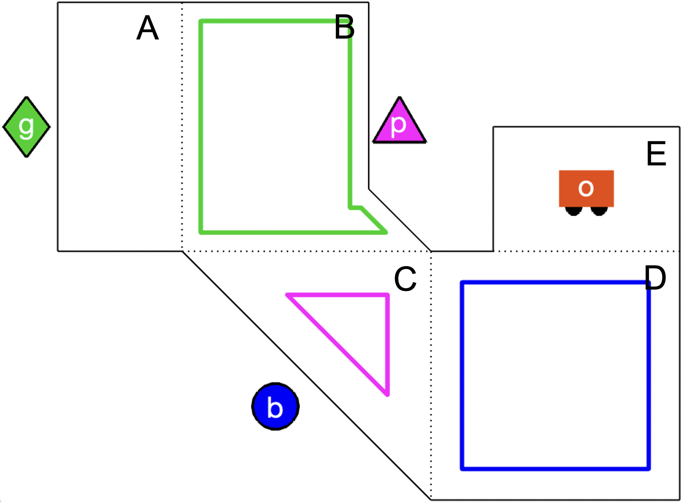
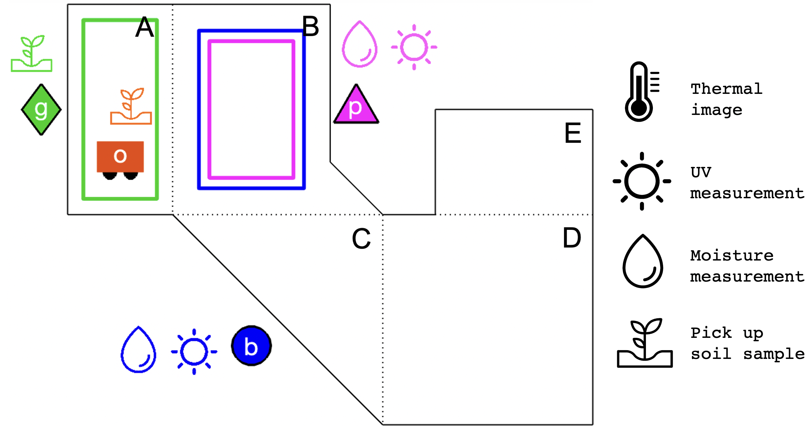
Example. Consider a group of four agents $A=\{A_{green}$ , $A_{blue}$ , $A_{orange}$ , $A_{pink}\}$ in a precision agriculture environment composed of 5 regions, as illustrated in Fig. 2. $A_{orange}$ is a mobile robot manipulator, such as Harvest Automation’s HV-100, while the other agents are stationary with different onboard sensing capabilities. The set of all capabilities is $\Lambda=\{$ $\lambda_{\mathit{area\_j}}$ , $\lambda_{motion}$ , $\lambda_{arm}$ , $\lambda_{UV}$ , $\lambda_{moisture}$ , $\lambda_{visual}$ , $\lambda_{thermal}\}$ , where $\forall j=\{green,blue,pink\}$ , $\lambda_{\mathit{area\_j}}$ is agent $j$ ’s sensing area model. The green agent can orient its arm to reach either region A or B. The blue agent can orient its sensors to see one of three regions, B, C, or D; in order to reorient its sensors from regions B to D, its sensing range must first pass through region C. Similarly, the pink agent can orient its sensors to see either region A, B, or C, and its sensing range must pass through region B to get from regions A to C. The orange agent’s ability to move between adjacent regions is represented by the capability $\lambda_{motion}$ . Its sensing region is whichever region it is in. $AP_{arm}=\{\textit{pickup, dropoff, weed}\}$ is an abstraction of a robot manipulator that represents different actions the arm can perform, such as picking up soil samples or pulling weeds. $AP_{UV}$ , $AP_{moisture}$ , $AP_{visual}$ , $AP_{thermal}$ all contain a single proposition representing a agent’s ability to take UV measurements, soil moisture measurements, visual images, and thermal images, respectively. $\lambda_{arm}$ has more states (see Fig. 1b). Each agent may have distinct cost functions corresponding to individual capabilities.

The agent capabilities and label on the initial state are:
$\Lambda_{green}=\{\lambda_{\mathit{area\_1}},\lambda_{\mathit{arm}}\},L(s_{0})=\{region_{B}\}$
$\Lambda_{blue}=\{\lambda_{\mathit{area\_2}},\lambda_{\mathit{moisture}},\lambda_{UV}\},L(s_{0})=\{region_{D}\}$
$\Lambda_{orange}=\{\lambda_{\mathit{motion}},\lambda_{\mathit{moisture}},\lambda_{UV},\lambda_{arm}\},L(s_{0})=\{region_{E}\}$
$\Lambda_{pink}=\{\lambda_{\mathit{area\_4}},\lambda_{\mathit{thermal}},\lambda_{\mathit{visual}},\lambda_{\mathit{moisture}},\lambda_{UV}\}$ , $L(s_{0})=\{region_{C}\}$

The team receives the task $\varphi^{\psi}$ (Eq. 4) and must determine a teaming assignment and behavior to satisfy the task. During execution, the agents must also synchronize with each other when necessary.

5. Approach

To find a teaming assignment and synthesize the corresponding synchronization and control, we first automatically generate a Büchi automaton $\mathcal{B}$ for the task $\varphi^{\psi}$ (Sec. 5.1). Each agent $A_{j}$ then constructs a product automaton $\mathcal{G}_{j}=A_{j}\times\mathcal{B}$ (Sec. 5.2). For each binding $\rho\in AP_{\psi}$ , it checks whether or not it can perform the task associated with that binding by finding a path to an accepting cycle in $\mathcal{G}_{j}$ . Each agent creates a copy of the Büchi automaton $\mathcal{B}_{j}$ pruned to remove any unreachable transitions and stores information about which combinations of binding assignments it can do.

For parts of the task that require collaboration (e.g., when a transition calls for actions with bindings $\{1,2\}$ and $r_{green}=\{1,2\},r_{blue}=\{2\}$ ), we need agents to synchronize. Thus, we synthesize behavior that allows for parallel execution while also guaranteeing that the team’s overall behavior satisfies the global specification.

To find a team of agents that can satisfy the task and their assignments, we need to guarantee that 1) every binding is assigned to at least one agent and 2) the agents synchronize for the collaborative portions of the task. To do so, we first run a depth-first search (DFS) to find a path through the $\mathcal{B}$ to an accepting cycle in which there exists a team of agents such that for every transition in the path, every proposition in $AP_{\psi}$ is assigned to at least one agent (Sec. 5.4). Each agent then synthesizes behavior to satisfy this path and communicates to other agents when synchronization is necessary.

5.1. Büchi Automaton for an LTL^ψ Formula

When constructing a Büchi automaton for an LTL^ψ specification, we automatically rewrite the specification such that the binding propositions are only over individual atomic proposition $\pi\in AP_{\varphi}$ (i.e. the formula is composed of $\pi^{\rho}$ ). For instance, the formula $(\neg pickup\ \mathcal{U}\ region_{A})^{1\vee 2}$ is rewritten as $(\neg pickup^{1}\ \mathcal{U}\ region_{A}^{1})\vee(\neg pickup^{2}\ \mathcal{U}\ region_{A}^{2}).$

In our running example, we rewrite the formula in Eq. 4a as

		$\displaystyle\Diamond(region_{B}^{2}\wedge moisture^{2}\wedge UV^{2}$		(5)
		$\displaystyle\wedge region_{B}^{3}\wedge moisture^{3}\wedge UV^{3}\wedge region_{A}^{1}\wedge pickup^{1})$

Remark 4. In rewriting the specification, negation follows bindings in the order of operations. For example, $\neg pickup^{1\wedge 2}=\neg pickup^{1}\wedge\neg pickup^{2}$ , and $\neg(pickup^{1\wedge 2})=\neg(pickup^{1}\wedge pickup^{2})=\neg(pickup^{1})\vee\neg(pickup^{2})$ .

From $AP_{\varphi}$ and $AP_{\psi}$ , we define the set of propositions $AP_{\varphi}^{\psi}$ , where $\forall\pi\in AP_{\varphi}$ and $\forall\rho\in AP_{\psi}$ , $\pi^{\rho}\in AP_{\varphi}^{\psi}$ . Given $AP_{\varphi}^{\psi}$ , we automatically translate the specification into a Büchi automaton using Spot Duret-Lutz et al. (2016).

To facilitate control synthesis, we transform any transitions in the Büchi automaton labeled with disjunctive formulas into disjunctive normal form (DNF). We then replace the transition labeled with a DNF formula containing $\ell$ conjunctive clauses with $\ell$ transitions between the same states, each labeled with a different conjunction of the original label.

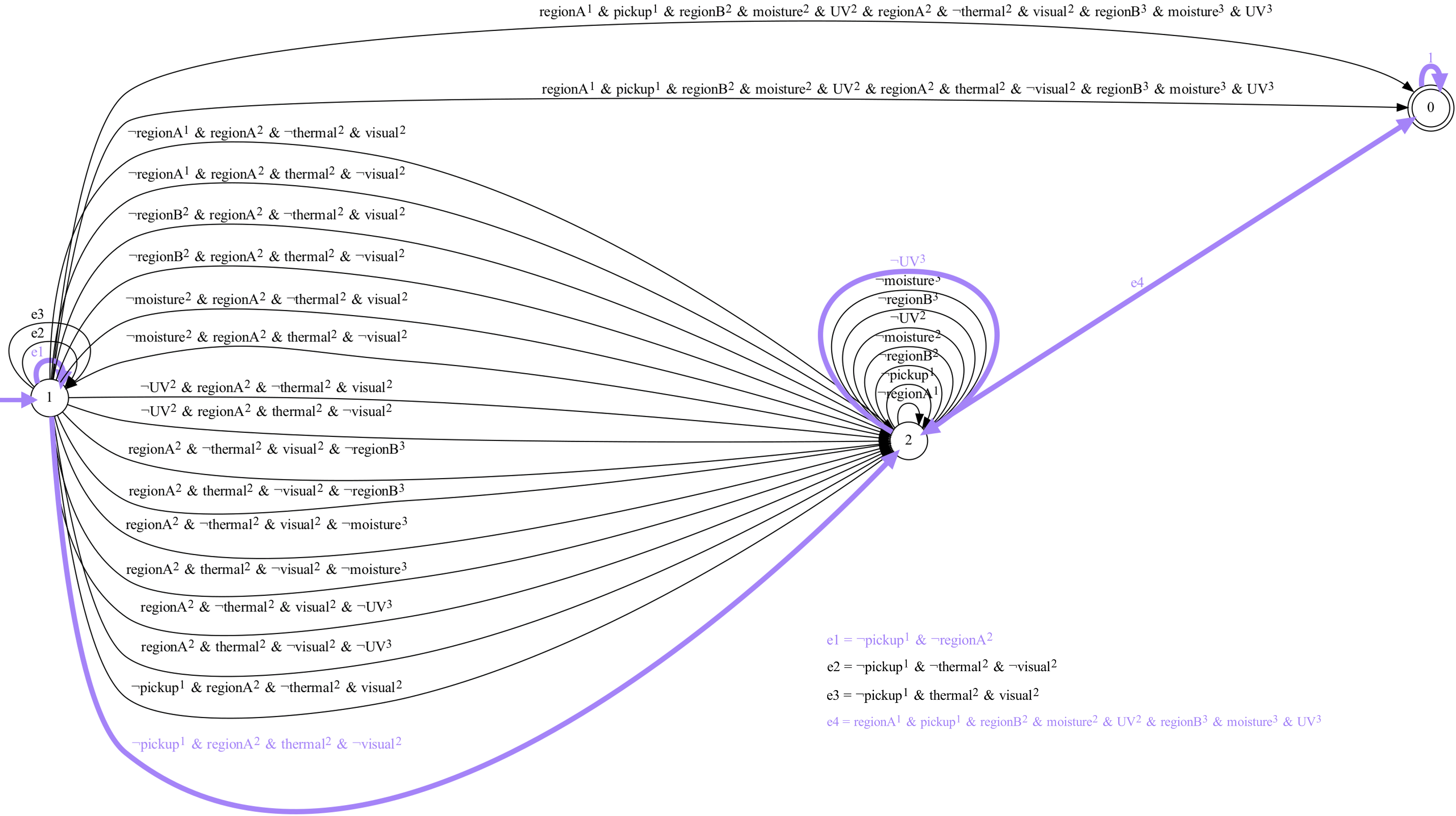
In general, when creating a Büchi automaton from an LTL formula $\varphi$ , $w\in\Sigma_{\mathcal{B}}$ are Boolean formulas over $AP_{\varphi}$ , the atomic propositions that appear in $\varphi$ , as seen in Fig. 3. In the following, for creating the product automaton, we use an equivalent representation, where $\Sigma_{\mathcal{B}}=2^{AP_{\varphi}^{\psi}}\times 2^{AP_{\varphi}^{\psi}}$ and $w=(\sigma_{T},\sigma_{F})\in\Sigma_{\mathcal{B}}$ contains the set of propositions that must be true, $\sigma_{T}$ , and the set of propositions that must be false, $\sigma_{F}$ , for the Boolean formula over a transition to evaluate to True. These sets are unique in our case since each transition is labeled with a conjunctive clause (i.e. no disjunction). Note that $\sigma_{T}\cap\sigma_{F}=\emptyset$ and $\sigma_{T}\cup\sigma_{F}\subseteq AP_{\varphi}$ ; propositions that do not appear in $w$ can have any truth value.

Given a Büchi automaton for an LTL^ψ specification $\mathcal{B}$ , we define the following functions:

Definition 1 (Binding Function). $\mathfrak{B}:\Sigma_{\mathcal{B}}\rightarrow 2^{AP_{\psi}}$ such that for $\sigma{=(\sigma_{T},\sigma_{F})}\in\Sigma_{\mathcal{B}},\mathfrak{B}(\sigma)\subseteq AP_{\psi}$ is the set $\{\rho\in AP_{\psi}\ |\ \exists\pi^{\rho}\in{\sigma_{T}\cup\sigma_{F}\}}$ . Intuitively, it is the set of bindings that appear in label $\sigma$ of a Büchi transition.

Definition 2 (Capability Function). $\mathfrak{C}:\Sigma_{\mathcal{B}}\times AP_{\psi}\rightarrow 2^{AP_{\varphi}}\times 2^{AP_{\varphi}}$ such that for $\sigma=(\sigma_{T},\sigma_{F})\in\Sigma_{\mathcal{B}},\rho\in AP_{\psi}$ , $\mathfrak{C}(\sigma,\rho)=(C_{T},C_{F})$ , where $C_{T}=\{\pi\in AP_{\varphi}\ |\ \exists\pi^{\rho}\in\sigma_{T}\}$ and $C_{F}=\{\pi\in AP_{\varphi}\ |\ \exists\pi^{\rho}\in\sigma_{F}\}$ . Here, $C_{T}$ and $C_{F}$ are the sets of action propositions that are True/False and appear with binding $\rho$ in label $\sigma$ of a Büchi transition.

5.2. Agent Behavior for an LTL^ψ Specification

To synthesize behavior for an agent, we find an accepting trace in its product automaton $\mathcal{G}_{j}=A_{j}\times\mathcal{B}$ , where $A_{j}=(S,s_{0},AP_{j},\gamma,L,W)$ is the agent model, and $\mathcal{B}=(Z,z_{0},\Sigma_{\mathcal{B}},\delta_{\mathcal{B}},F)$ is the Büchi automaton.

Since the set of propositions of $A_{j}$ may not be equivalent to the set of propositions of $\mathcal{B}$ , we borrow from the definition of the product automaton in Fang and Kress-Gazit (2022). We first define the following function:

Definition 3 (Binding Assignment Function). Let $q=(s,z)$ , $q^{\prime}=(s^{\prime},z^{\prime})$ , $\sigma=(\sigma_{T},\sigma_{F})\in\Sigma_{\mathcal{B}}$ . Then $\mathfrak{R}(q,\sigma,q^{\prime})=\{r\in 2^{AP_{\psi}}\setminus\emptyset\ |\ \forall\rho\in r,(C_{T},C_{F})=\mathfrak{C}(\sigma,\rho),\bigcup_{\rho\in r}C_{T}\subseteq L(s^{\prime})$ and $\bigcup_{\rho\in r}C_{F}\cap L(s^{\prime})=\emptyset\}$ .

Intuitively, $\mathfrak{R}$ outputs all possible combinations of binding propositions that the agent can be assigned for a transition $(q,\sigma,q^{\prime})$ . An agent can be assigned $\rho$ if and only if the agent’s next state $s^{\prime}$ is labeled with all the action and motion propositions $\pi\in AP_{\varphi}$ that appear in $\sigma_{T}$ as $\pi^{\rho}$ , and all the propositions $\pi\in AP_{\varphi}$ that appear in $\sigma_{F}$ as $\pi^{\rho}$ are not part of the state label (i.e. the agent is not performing that action). If a proposition $\pi^{\rho}$ is in $\sigma_{F}$ and $\pi$ is not in $AP_{j}$ (e.g. $scan^{1}\in\sigma_{F}$ and the agent does not have $\lambda_{scan}$ ), the agent may be assigned $\rho$ . Note that $r$ may include any binding propositions that are not in $\sigma$ , since there are no actions required by those bindings in that transition. For example, if $\sigma=(\{scan^{1}\},\{pickup^{2}\})$ and $AP_{\psi}=\{1,2,3\}$ , then $\{3\}$ will be in the set $\mathfrak{R}(q,\sigma,q^{\prime})$ for all $q,q^{\prime}$ .

Given $A_{j}$ and $\mathcal{B}$ , we define the product automaton $\mathcal{G}_{j}=A_{j}\times\mathcal{B}$ :

Definition 4 (Product Automaton). The product automaton $\mathcal{G}_{j}=(Q,q_{0},AP_{j},\delta_{\mathcal{G}},L_{\mathcal{G}},W_{\mathcal{G}},F_{\mathcal{G}})$ , where

•

$Q=S\times Z$ is a finite set of states
•

$q_{0}=(s_{0},z_{0})\in Q$ is the initial state
•

$\delta_{\mathcal{G}}\subseteq Q\times Q$ is the transition relation, where for $q=(s,z)$ and $q^{\prime}=(s^{\prime},z^{\prime})$ , $(q,q^{\prime})\in\delta_{\mathcal{G}}$ if and only if $(s,s^{\prime})\in\gamma$ and $\exists\sigma\in\Sigma_{\mathcal{B}}$ such that $(z,\sigma,z^{\prime})\in\delta_{\mathcal{B}}$ and $\mathfrak{R}(q,\sigma,q^{\prime})\neq\emptyset$
•

$L_{\mathcal{G}}$ is the labeling function s.t. for $q=(s,z)$ , $L_{\mathcal{G}}(q)\!=\!L(s)\!\subseteq\!AP_{j}$
•

$W_{\mathcal{G}}:\delta_{\mathcal{G}}\rightarrow\mathbb{R}_{\geq 0}$ is the cost function s.t. for $(q,q^{\prime})\in\delta_{\mathcal{G}}$ , $q=(s,z)$ , $q^{\prime}=(s^{\prime},z^{\prime})$ , $W_{\mathcal{G}}((q,q^{\prime}))=W((s,s^{\prime}))$
•

$F_{\mathcal{G}}=S\times F$ is the set of accepting states

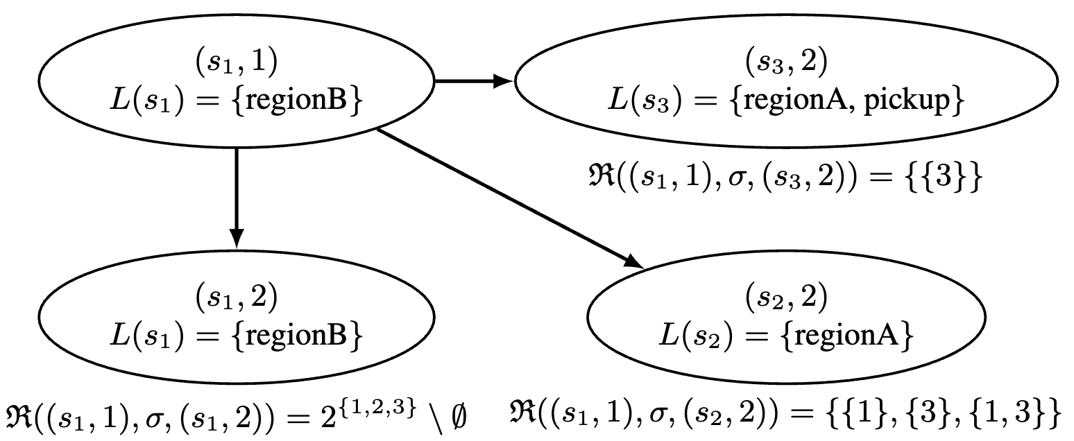
Example. Fig. 4 depicts a small portion of $\mathcal{G}_{green}$ ; for the self-transition in $\mathcal{B}$ that is labeled with $\sigma=(\emptyset$ , $\{pickup^{1},$ $region_{A}^{2}\})$ (labeled as $e1$ in Fig. 3), and for states in $A_{green}$ where $L(s_{1})=\{region_{B}\}$ , $L(s_{2})=\{region_{A}\}$ , $L(s_{3})=\{region_{A},pickup\}$ , then the possible binding assignments are $\mathfrak{R}((s_{1},1),\sigma,(s_{1},2))=2^{\{1,2,3\}}\setminus\emptyset$ and $\mathfrak{R}((s_{1},1),\sigma,(s_{2},2))=\{\{1\},\{3\},\{1,3\}\}$ . When the agent is in $s_{3}$ , it cannot be assigned either bindings 1 or 2, but since no propositions appear with binding 3 in $\sigma$ , $\mathfrak{R}((s_{1},1),\sigma,(s_{3},2))=\{\{3\}\}$ .

5.3. Finding Possible Individual Agent Bindings

To construct a team, we first reason about each agent and the sets of bindings it can perform. For example, for a formula $region_{A}^{1}\wedge region_{B}^{2}$ , an agent may be assigned $r_{j}=\{1\}$ or $r_{j}=\{2\}$ but not $r_{j}=\{1,2\}$ , since it cannot be in two regions at the same time.

To find the set of possible binding assignments $R_{j}\subseteq 2^{AP_{\psi}}$ , we search for an accepting trace in $\mathcal{G}_{j}$ for every binding assignment $r_{j}\in 2^{AP_{\psi}}$ . We start from the full set of bindings $r_{j}=AP_{\psi}$ . Given an assignment $r_{j}$ to check, we find an accepting trace in $\mathcal{G}_{j}$ such that for all transitions $(q,q^{\prime})$ in the trace, $r_{j}\subseteq\mathfrak{R}(q,\sigma,q^{\prime})$ . This ensures that the agent can satisfy its binding assignment for the entirety of its execution (i.e. $r_{j}$ does not change). Since every subset of a binding assignment $r_{j}$ is itself a possible binding assignment, if the agent can be assigned all $m=|AP_{\psi}|$ bindings, then we know it can also be assigned every possible subset of $m$ . If not, we check the ${m\choose m-1}$ combinations, and continue iterating until we have determined the agent’s ability to perform every combination of the $m$ bindings.

Once an agent determines its possible binding assignments $R_{j}$ , it creates the Büchi automaton $\mathcal{B}_{j}$ by removing any transition in $\mathcal{B}$ that cannot be traversed by any assignment in $R_{j}$ . In our example (Fig. 3), each agent can be assigned at least one binding over every transition in $\mathcal{B}$ . Thus, $\forall j\in\{green,blue,orange,pink\},\mathcal{B}_{j}=\mathcal{B}$ .

5.4. Agent Team Assignment

A team of agents can perform the task if 1) all the bindings are assigned, with each agent maintaining the same binding assignment for the entirety of the task, and 2) the agents satisfy synchronization requirements. For a viable team, the agents’ control follows the same path in the Büchi automaton $\mathcal{B}$ to an accepting cycle. We perform DFS over $\mathcal{B}$ to find an accepting trace (Alg. 1), where each tuple in $stack$ contains the current edge $(z,\sigma,z^{\prime})$ , the current team of agents $R_{\hat{A}}$ , and the path traversed so far $\beta_{\hat{A}}$ .

We initialize the team with all agents $A_{j}$ and all possible binding assignments $R_{j}$ , and each path $\beta_{\hat{A}}$ starts from state $z_{0}$ of $\mathcal{B}$ . When checking a transition $(z,\sigma,z^{\prime})$ , we remove any agent $j$ if $\forall((s,z),(s^{\prime},z^{\prime}))\in\delta_{\mathcal{G}_{j}}$ , there are no possible binding assignments it can satisfy. This is done by checking each agent’s pruned Büchi automaton $\mathcal{B}_{j}$ in update_team (line 1). We want the agent’s behavior to satisfy not only the current transition, but also the entire path with a consistent binding assignment. Thus, we update possible bindings (update_bindings, lines 1-1).

To guarantee the overall team behavior, we need to ensure agents are able to “wait in a state” before they synchronize, as they may reach states at different times. This means that each state in the trace must have a corresponding self-transition. Thus, for every $(z,\sigma,z^{\prime})$ that we add to the path in which $z\neq z^{\prime}$ , the next edge to traverse must be a self-transition from $z^{\prime}$ to itself; the same holds vice-versa. In line 1, we check if the current transition is self-looping or not, and add subsequent transitions into the stack accordingly. If there is no self-transition on $z^{\prime}$ (i.e. $(z^{\prime},\sigma,z^{\prime})\notin\delta_{\mathcal{B}}$ ), then we do not consider $z^{\prime}$ to be valid and do not add it to the path.

Once we find a valid path to an accepting cycle, we parse it into $\beta$ , the path without self-transitions, and $\delta_{self}$ , which contains the corresponding self-transition for each state in the path. Fig. 3 shows a valid path in $\mathcal{B}$ for the example in Sec. 4 and the corresponding team assignment $\hat{A}=\{A_{green},A_{blue},A_{orange},A_{pink}\}$ and bindings $r_{green}=\{1\}$ , $r_{blue}=\{3\},r_{orange}=\{1\},r_{pink}=\{2,3\}$ . Note that we find a valid path rather than a globally optimal one. However, the algorithm is complete; it will find a feasible path if one exists.

Input :

A=\{A_{1},A_{2},...,A_{n}\}

R=\{R_{1},R_{2},...,R_{n}\}

\mathcal{B}

\{\mathcal{B}_{1},\mathcal{B}_{2}...,\mathcal{B}_{n}\}

Output :

\beta

\delta_{self}

\hat{A}\subseteq A

R_{\hat{A}}

stack=\emptyset

visited=\emptyset

3 for

e\in\{(z,\sigma,z^{\prime})\in\delta_{\mathcal{B}}\ |\ z=z_{0}\}

stack=stack\cup\{(e,R,[e])\}

5while

stack\neq\emptyset

((z,\sigma,z^{\prime}),R_{\hat{A}},\beta_{\hat{A}})=stack.pop()

8 if

(z,\sigma,z^{\prime})\not\in visited

then

visited=visited\cup(z,\sigma,z^{\prime})

R_{\hat{A}}=\textsc{update\_team}((z,\sigma,z^{\prime}),\{\mathcal{B}_{1},...,\mathcal{B}_{n}\})

12 for

R_{j}\in R_{\hat{A}}

R_{j}^{\prime}=\textsc{update\_bindings}(R_{j},(z,\sigma,z^{\prime}))

14 if

R_{j}^{\prime}=\emptyset

then

R_{\hat{A}}=R_{\hat{A}}\setminus R_{j}

16 else

R_{\hat{A}}=(R_{\hat{A}}\setminus R_{j})\cup R_{j}^{\prime}

19 if

\bigcup_{j}(R_{j}\in R_{\hat{A}})=AP_{\psi}

then

21 if

z^{\prime}\in F

then

\beta,\delta_{self}=\textsc{parse\_path}(\beta_{\hat{A}})

23 return

\beta,\delta_{self},R_{\hat{A}}

E=\{(z^{\prime},\sigma^{\prime},z^{\prime\prime})\in\delta_{\mathcal{B}}\}

25 for

(z^{\prime},\sigma^{\prime},z^{\prime\prime})\in E

26 if

(z=z^{\prime}\text{ and }z^{\prime}\neq z^{\prime\prime})

(z\neq z^{\prime}\text{ and }z^{\prime}=z^{\prime\prime})

then

stack=stack\cup\{\left((z^{\prime},\sigma^{\prime},z^{\prime\prime}),R_{\hat{A}},[\beta_{\hat{A}}\ (z^{\prime},\sigma^{\prime},z^{\prime\prime})]\right)\}

Algorithm 1 Find Accepting Trace for Agent Team

5.5. Synthesis and Execution of Control and Synchronization Policies

Given an accepting trace $\beta$ through $\mathcal{B}$ and the corresponding self-transitions $\delta_{self}$ that are valid for all agents in $R_{\hat{A}}$ , we synthesize control and synchronization for each agent such that the overall team execution satisfies $\beta$ (Alg. 2). For each transition $(z,\sigma,z^{\prime})$ in $\beta$ , we find $\overline{R}$ , which contains the binding assignments of all agents that require synchronization at state $z^{\prime}$ . Agent $j$ participates in the synchronization step if $r_{j}$ contains a binding $\rho$ that is required by $\sigma$ and is not the only agent assigned bindings from $\sigma$ (line 2).

Subsequently, agent $j$ finds an accepting trace in $\mathcal{G}_{j}$ that reaches $z^{\prime}$ with minimum cost, following self-transitions stored in $\delta_{self}$ if necessary. As it executes this behavior, it communicates with other agents the tuple $p$ , which contains 1) its ID, 2) the state $z^{\prime}$ it is currently going to, and 3) if it is ready for synchronization (line 2). If no synchronization is required (line 2), the agent can simply execute the behavior. Otherwise, to guarantee that the behavior does not violate the requirements of the task, the agent executes the synthesized behavior up until the penultimate state, $z_{wait}$ .

When the agent reaches $z_{wait}$ , it signals to other agents that it is ready for synchronization. Since all agents know the overall teaming assignment, the agent continues to wait in state $z_{wait}$ until it receives a signal that all other agents in $\overline{R}$ are ready (line 2). These agents then move to the next state in the behavior simultaneously. Agent $j$ continues synthesizing behavior through $\beta$ until synchronization is necessary again, and this process is repeated.

Input :

\mathcal{G}_{j}

r_{j}

R_{\hat{A}}

\beta

\delta_{self}

1 for

(z,\sigma,z^{\prime})\in\beta

b_{j}=\textsc{find\_behavior}(\mathcal{G}_{j},r_{j},(z,\sigma,z^{\prime}),\delta_{self})

\overline{R}=\{r_{k}\in R_{\hat{A}}\ |\ r_{k}\cap\mathfrak{B}(\sigma)\neq\emptyset\}

r_{j}\not\in\overline{R}

\overline{R}=\{r_{j}\}

then

p=()

\textsc{execute}(b_{j},p)

6 else

p=(j,z^{\prime},0)

\ell=length(b_{j})

\textsc{execute}(b_{j}[1:\ell-1],p)

z_{wait}=b_{j}[\ell-1]

P=\{j\}

10 while

\bigcup_{i\in P}(r_{i}\in\overline{R})\neq\mathfrak{B}(\sigma)

p=(j,z^{\prime},1)

\textsc{execute}(z_{wait},p)

P=j\cup\{k\ |\ (k,z^{\prime},1)\in\textsc{receive}()\}

\textsc{execute}(b_{j}[\ell])

Algorithm 2 Synthesize an Agent’s Behavior

6. Results and Discussion

Fig. 5 shows the final step of the synchronized behavior of the agent team for the example in Section 4, where $\hat{A}=\{$ $A_{green}$ , $A_{blue}$ , $A_{orange}$ , $A_{pink}\}$ with binding assignments $r_{green}=\{1\}$ , $r_{blue}=\{3\},r_{orange}=\{1\},r_{pink}=\{2,3\}$ . A simulation of the full behavior is shown in the accompanying video.

Optimizing teams: Our synthesis algorithm can be seen as a greatest fixpoint computation, where we start with the full set of agents and remove those that cannot contribute to the task. As a result, the team may have redundancies, i.e. agents can be removed while still ensuring the overall task will be completed; this may be beneficial for robustness. Furthermore, we can choose a sub-team to optimize different metrics, as long as the agent bindings assignments still cover all the required bindings. For example, minimizing the number of bindings per agent could result in $\hat{A}=\{A_{green},A_{blue},A_{pink}\}$ , $r_{green}=\{1\},r_{blue}=\{3\},r_{pink}=\{2\}$ ; minimizing the number of agents results in $\hat{A}=\{A_{green},A_{pink}\}$ , $r_{green}=\{1\},r_{pink}=\{2,3\}$ .

To illustrate other possible metrics, we consider a set of 20 agents and create a team for the specification in Eq. 4. Their final binding assignments and costs are shown in Table 1. Minimizing cost results in a team $\hat{A}=\{A_{7},A_{11}\}$ . Minimizing cost while requiring each binding to be assigned to two agents results in $\hat{A}=\{A_{4},A_{7},A_{11},A_{16}\}$ .

Agent	$r_{j}$	$cost$	Agent	$r_{j}$	$cost$	Agent	$r_{j}$	$cost$	Agent	$r_{j}$	$cost$	Agent	$r_{j}$	$cost$
1	1	1.2	5	3	2.75	9	3	2.6	13	3	2.0	17	2,3	3.275
2	3	1.0	6	1	0.95	10	1	2.8	14	1	1.2	18	3	2.55
3	1	1.2	7	1	0.65	11	2,3	0.9	15	3	1.1	19	1	1.9
4	2,3	1.3	8	1	1.0	12	2,3	1.825	16	1	0.775	20	2,3	2.35

Table 1. Example teaming assignment with 20 robots

Computational complexity: The control synthesis algorithm (Alg. 2) is agnostic to the number of agents, since each agent determines its own possible bindings assignments and behavior. For the team assignment (Alg. 1), since it is a DFS algorithm, we need to store the agent team and their possible binding assignments as we build an accepting trace. Thus, it has both a space and time complexity of $O(|E|*2^{m}*n)$ , where $|E|$ is the number of edges in $\mathcal{B}$ , $m$ is the number of bindings, and $n$ is the number of agents.

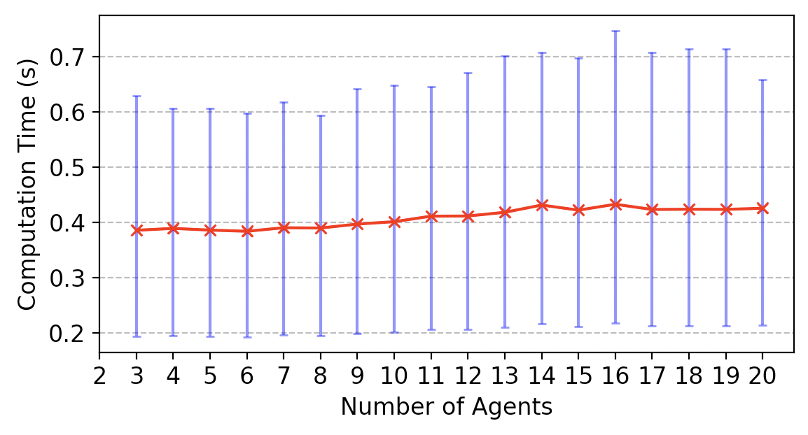
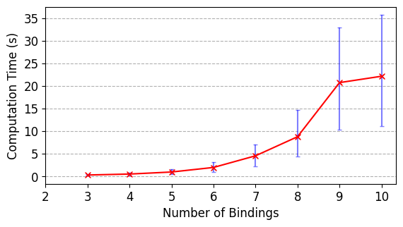
Fig. 6(a) shows the computation time of the synthesis framework (Sec. 5.2 – 5.4) for simulated agent teams in which we vary the number of agents from 3 to 20, running 30 simulations for each set of agents and randomizing their capabilities. The task for each simulation is the example in Eq. 4. We also ran simulations in which we increase the number of bindings from 3 to 10 and randomized the capabilities of 4 agents (Fig. 6(b)). The variance in computation time is a result of the randomized agent capabilities, which affects the computation time of possible binding assignments (Sec. 5.3). All simulations ran on a 2.5 GHz quad-core Intel Core i7 CPU.

Task expressivity with respect to other approaches: We compare LTL^ψ to other approaches that encode collaborative heterogeneous multi-agent tasks using temporal logic.

Standard LTL: One approach is to use LTL to express the task by enumerating all possible assignments in the specification. In our example, Eq. 4a would be rewritten as:

	$\displaystyle\varphi^{\psi}_{1}=$	$\displaystyle(\Diamond((region_{B}^{green}\wedge moisture^{green}\wedge UV^{green})$
	$\displaystyle\wedge$	$\displaystyle(region_{A}^{blue}\wedge pickup^{blue})))$
	$\displaystyle\vee$	$\displaystyle(\Diamond((region_{B}^{green}\wedge moisture^{green}\wedge UV^{green})$
	$\displaystyle\wedge$	$\displaystyle(region_{A}^{orange}\wedge pickup^{orange})))\vee...$

where each agent has its own unique set of $AP$ , denoted here by each proposition’s superscript. As a result, the number of propositions increases exponentially with the number of agents. The task complexity also increases, as the specification must include all possible agent assignments. Another drawback of using LTL for such tasks is that the specification is not generalizable to any number of agents; it must be rewritten when the set of agents change.

LTL^χ: In Luo and Zavlanos (2022), tasks are written in LTL^χ, where proposition $\pi_{i,j}^{k,\chi}$ is true if at least $i$ agents of type $j$ are in region $k$ with binding $\chi$ . We can express $\varphi^{\psi}_{1}$ (Eq. 4a) of our example as $\Diamond(\pi_{1,mois}^{regionB,2}\wedge\pi_{1,UV}^{regionB,2}\wedge\pi_{1,mois}^{regionB,3}\wedge\pi_{1,UV}^{regionB,3}\wedge\pi_{1,arm}^{regionA,1})$ . The truth value of $\pi_{i,j}^{k,\chi}$ is not dependent on any particular action an agent might take. LTL^χ can be extended to action propositions, but since an agent can only be categorized as one type, each type of agent must have non-overlapping capabilities (here, we have written the LTL^χ formula such that each type of agent only has one capability). In addition, $\varphi^{\psi}_{2}$ (Eq. 4b) cannot be written in LTL^χ because the negation defined in our grammar cannot be expressed in LTL^χ. On the other hand, the negative proposition $\neg\pi_{i,j}^{k,\chi}$ from Luo and Zavlanos (2022) is equivalent to “less than $i$ agents of type $j$ are in region $k$ ”, which our logic cannot encode.

Capability Temporal Logic (CaTL): Tasks in CaTL Leahy et al. (2022) are constructed over tasks $T=(d,\pi,cp_{T})$ , where $d$ is a duration of time, $\pi$ is a region in AP, $(c_{i},m_{i})\in cp_{T}$ denotes that at least $m_{i}$ agents with capability $c_{i}$ are required. Similar to our grammar, CaTL allows agents to have multiple capabilities, but each task must specify the number of agents required. Since it is an extension of Signal Temporal Logic, tasks provide timing requirements, which our logic cannot encode. However, it does not include the concept of binding assignments; in our example $\varphi^{\psi}_{1}$ (Eq. 4a), CaTL cannot express that we require the same agent that took a UV measurement to also take a thermal image. Ignoring binding assignments and adding timing constraints, $\varphi^{\psi}_{1}$ (Eq. 4a) can be rewritten in CaTL as $\Diamond_{[0,10)}$ $(T(0.1,region_{B},$ $\{(moisture,2),(UV,2)\})\wedge$ $T(0.5,$ $region_{A},$ $\{(arm,1)\})$ . Each capability in CaTL is represented as a sensor and therefore cannot include more complex capabilities, such as a robot arm that can perform several different actions. In addition, because CaTL requires the formula to be in positive normal form (i.e. no negation), we cannot express $\varphi^{\psi}_{2}$ (Eq. 4b) in this grammar.

7. Conclusion

We define a new task grammar for heterogeneous teams of agents and develop a framework to automatically assign the task to a (sub)team of agents and synthesize correct-by-construction control policies to satisfy the task. We include synchronization constraints to guarantee that the agents perform the necessary collaborations.

In future work, we plan to demonstrate the approach on physical systems where we need to ensure that the continuous execution satisfies all the collaboration and safety constraints. In addition, we will explore different notions of optimality when finding a teaming plan, as well as increase the expressivity of the grammar by allowing reactive tasks where agents modify their behavior at runtime in response to environment events.

{acks}

This work is supported by the National Defense Science & Engineering Graduate Fellowship (NDSEG) Fellowship Program.

References

(1)
Baier and Katoen (2008) Christel Baier and Joost-Pieter Katoen. 2008. Principles of Model Checking. The MIT Press.
Chen et al. (2021) Ji Chen, Ruojia Sun, and Hadas Kress-Gazit. 2021. Distributed Control of Robotic Swarms from Reactive High-Level Specifications. In 2021 IEEE 17th International Conference on Automation Science and Engineering (CASE). 1247–1254. https://doi.org/10.1109/CASE49439.2021.9551578
Chen et al. (2011) Yushan Chen, Xu Chu Ding, and Calin Belta. 2011. Synthesis of distributed control and communication schemes from global LTL specifications. In 2011 50th IEEE Conference on Decision and Control and European Control Conference. 2718–2723. https://doi.org/10.1109/CDC.2011.6160740
Duret-Lutz et al. (2016) Alexandre Duret-Lutz, Alexandre Lewkowicz, Amaury Fauchille, Thibaud Michaud, Etienne Renault, and Laurent Xu. 2016. Spot 2.0 — a framework for LTL and $\omega$ -automata manipulation. In Proceedings of the 14th International Symposium on Automated Technology for Verification and Analysis (ATVA’16) (Lecture Notes in Computer Science, Vol. 9938). Springer, 122–129. https://doi.org/10.1007/978-3-319-46520-3_8
Emerson (1990) E. Allen Emerson. 1990. Temporal and Modal Logic. In Formal Models and Semantics, JAN Van Leeuwen (Ed.). Elsevier, Amsterdam, 995–1072. https://doi.org/10.1016/B978-0-444-88074-1.50021-4
Fang and Kress-Gazit (2022) Amy Fang and Hadas Kress-Gazit. 2022. Automated Task Updates of Temporal Logic Specifications for Heterogeneous Robots. In 2022 International Conference on Robotics and Automation (ICRA). 4363–4369. https://doi.org/10.1109/ICRA46639.2022.9812045
Faruq et al. (2018) Fatma Faruq, David Parker, Bruno Laccrda, and Nick Hawes. 2018. Simultaneous Task Allocation and Planning Under Uncertainty. In 2018 IEEE/RSJ International Conference on Intelligent Robots and Systems (IROS). 3559–3564. https://doi.org/10.1109/IROS.2018.8594404
Gerkey and Matarić (2004) Brian P. Gerkey and Maja J. Matarić. 2004. A Formal Analysis and Taxonomy of Task Allocation in Multi-Robot Systems. The International Journal of Robotics Research 23, 9 (2004), 939–954. https://doi.org/10.1177/0278364904045564 arXiv:https://doi.org/10.1177/0278364904045564
Jia and Meng (2013) Xiao Jia and Max Q.-H. Meng. 2013. A survey and analysis of task allocation algorithms in multi-robot systems. In 2013 IEEE International Conference on Robotics and Biomimetics (ROBIO). 2280–2285. https://doi.org/10.1109/ROBIO.2013.6739809
Kantaros and Zavlanos (2020) Yiannis Kantaros and Michael M Zavlanos. 2020. STyLuS*: A Temporal Logic Optimal Control Synthesis Algorithm for Large-Scale Multi-Robot Systems. The International Journal of Robotics Research 39, 7 (2020), 812–836. https://doi.org/10.1177/0278364920913922 arXiv:https://doi.org/10.1177/0278364920913922
Kloetzer and Belta (2010) Marius Kloetzer and Calin Belta. 2010. Automatic Deployment of Distributed Teams of Robots From Temporal Logic Motion Specifications. IEEE Transactions on Robotics 26, 1 (2010), 48–61. https://doi.org/10.1109/TRO.2009.2035776
Korsah et al. (2013) G. Ayorkor Korsah, Anthony Stentz, and M. Bernardine Dias. 2013. A comprehensive taxonomy for multi-robot task allocation. The International Journal of Robotics Research 32, 12 (2013), 1495–1512. https://doi.org/10.1177/0278364913496484 arXiv:https://doi.org/10.1177/0278364913496484
Leahy et al. (2022) Kevin Leahy, Zachary Serlin, Cristian-Ioan Vasile, Andrew Schoer, Austin M. Jones, Roberto Tron, and Calin Belta. 2022. Scalable and Robust Algorithms for Task-Based Coordination From High-Level Specifications (ScRATCHeS). IEEE Transactions on Robotics 38, 4 (2022), 2516–2535. https://doi.org/10.1109/TRO.2021.3130794
Li et al. (2009) Zhiyong Li, Bo Xu, Lei Yang, Jun Chen, and Kenli Li. 2009. Quantum Evolutionary Algorithm for Multi-Robot Coalition Formation. In Proceedings of the First ACM/SIGEVO Summit on Genetic and Evolutionary Computation (Shanghai, China) (GEC ’09). Association for Computing Machinery, New York, NY, USA, 295–302. https://doi.org/10.1145/1543834.1543874
Luo and Zavlanos (2022) Xusheng Luo and Michael M. Zavlanos. 2022. Temporal Logic Task Allocation in Heterogeneous Multirobot Systems. IEEE Transactions on Robotics (2022), 1–20. https://doi.org/10.1109/TRO.2022.3181948
Sahin et al. (2017) Yunus Emre Sahin, Petter Nilsson, and Necmiye Ozay. 2017. Synchronous and asynchronous multi-agent coordination with cLTL+ constraints. In 2017 IEEE 56th Annual Conference on Decision and Control (CDC). 335–342. https://doi.org/10.1109/CDC.2017.8263687
Schillinger et al. (2018) Philipp Schillinger, Mathias Bürger, and Dimos V. Dimarogonas. 2018. Simultaneous task allocation and planning for temporal logic goals in heterogeneous multi-robot systems. The International Journal of Robotics Research 37, 7 (2018), 818–838. https://doi.org/10.1177/0278364918774135 arXiv:https://doi.org/10.1177/0278364918774135
Schmickl et al. (2006) Thomas Schmickl, Christoph Möslinger, and Karl Crailsheim. 2006. Collective Perception in a Robot Swarm. 144–157. https://doi.org/10.1007/978-3-540-71541-2_10
Tumova and Dimarogonas (2016) Jana Tumova and Dimos V. Dimarogonas. 2016. Multi-agent planning under local LTL specifications and event-based synchronization. Automatica 70 (2016), 239–248. https://doi.org/10.1016/j.automatica.2016.04.006
Ulusoy et al. (2012) Alphan Ulusoy, Stephen L. Smith, Xu Chu Ding, and Calin A. Belta. 2012. Robust multi-robot optimal path planning with temporal logic constraints. 2012 IEEE International Conference on Robotics and Automation (2012), 4693–4698.
Wang and Rubenstein (2020) Hanlin Wang and Michael Rubenstein. 2020. Shape Formation in Homogeneous Swarms Using Local Task Swapping. IEEE Transactions on Robotics 36, 3 (2020), 597–612. https://doi.org/10.1109/TRO.2020.2967656
Xu et al. (2015) Bo Xu, Zhaofeng Yang, Yu Ge, and Zhiping Peng. 2015. Coalition Formation in Multi-agent Systems Based on Improved Particle Swarm Optimization Algorithm. International Journal of Hybrid Information Technology 8 (03 2015), 1–8. https://doi.org/10.14257/ijhit.2015.8.3.01

High-Level, Collaborative Task Planning Grammar and Execution for Heterogeneous Agents

Abstract.

Key words and phrases:

1. Introduction

2. Preliminaries

2.1. Linear Temporal Logic

2.2. Büchi Automata

2.3. Agent Model

3. Task Grammar - LTLψ

4. Control Synthesis for LTLψ

5. Approach

5.1. Büchi Automaton for an LTLψ Formula

5.2. Agent Behavior for an LTLψ Specification

5.3. Finding Possible Individual Agent Bindings

5.4. Agent Team Assignment

5.5. Synthesis and Execution of Control and Synchronization Policies

6. Results and Discussion

7. Conclusion

References

3. Task Grammar - LTL^ψ

4. Control Synthesis for LTL^ψ

5.1. Büchi Automaton for an LTL^ψ Formula

5.2. Agent Behavior for an LTL^ψ Specification