High-Fidelity Semianalytical Theory for a Low Lunar Orbit
1 Introduction
Since the 1990s, there has been a renewed interest in the exploration of the Moon. A significant number of lunar missions have been and are being conducted by the United States of America, Russia, Europe, Japan, India, and China. Most of these missions require low-altitude orbits. For this reason, looking for ideal orbits that minimize or cancel the undesirable effects of some perturbations which can modify spacecraft orbits continue to be a current problem. Classically, these ideal orbits have been known as frozen orbits. A historical review of the frozen-orbit concept can be found in [1] and the references cited therein.
Basically, from the mathematical point of view, a frozen orbit corresponds to an equilibrium of a system of differential equations in which the influence of the short- and medium-period terms has been removed. The reduced or double-averaged system only maintains the long-period dynamics. This system of differential equations can be derived in two ways. First, the problem can be formulated using the well-known Lagrange planetary equations, where the short- and medium-period terms can be removed by classical averaging techniques [2, 3, 4, 5, 6, 7, 8]. Second, the problem can also be expressed in Hamiltonian form, in which case the elimination process can be carried out by sophisticated methods based on Lie transforms [1, 9, 10, 11], which allow determining easily the transformations between mean and osculating elements.
In general, these ideas have been employed extensively for mission-design studies. When they are applied to the case of an orbiter around the Earth, only a few zonal harmonic coefficients of the Earth’s gravitational potential are enough to allow characterizing the phase-space structure of the full problem [1]. However, in the case of real mission-design analyses of low lunar orbiters, it is necessary to consider a full perturbation model which must include both a high-resolution lunar gravitational-field model and the third-body attraction caused by the Earth [12]. As a reference, Roncoli [13] recommends a lunar gravitational-field model as the minimum for orbits with altitudes below 100 km, resolution later confirmed by Lara et al. in [10, 11].
In this context, we consider it necessary to revisit and extend the semi-analytical models developed in [14, 15], whose aim was to test the feasibility of perturbation theories based on Lie transforms, and therefore constituted mere academic proof-of-concept studies that served the author to develop specific software for this task444Using this software, results in [14] where later validated by the coworkers of the first author of this paper [16].. Indeed, since the first high-resolution lunar gravitational fields were released [17], it is well known that high-inclination, low-altitude lunar orbits behave quite differently from what lower-degree models predict.
In the present work, both the symbolic-manipulation software developed by the authors of this article and our expertise from previous models are applied to the analysis of an orbiter in a low-altitude near-circular orbit around the Moon, perturbed by the combined effect of a lunar gravitational-field model and the third-body attraction caused by the Earth. Our objective is to develop a semi-analytical theory that can be integrated both in a symbolic software tool for the computation of real low-altitude frozen orbits and in a semi-analytical propagator for low-altitude orbits. By means of two Lie transforms, we remove the short- and medium-period terms from the original problem. As a result, the double-averaged problem only depends on the argument of the periapsis, and then its long-term behavior can be studied. Finally, we analyze the influence of the zonal coefficients and the third-body attraction from the Earth in the phase-space structure of the double-averaged problem. The resulting analytical expressions can be used to locate frozen orbits in the double-averaged problem, as well as to perform all the required computations in order to transform the frozen conditions into a near-periodic orbit for the original problem.
2 Dynamical model
The following Hamiltonian describes the motion of an orbiter around the Moon, perturbed by its gravitational force, , and by the third-body attraction due to the Earth , under the Hill hypothesis, that is, assuming that the Moon is in circular orbit around the Earth and that the Earth is moving in a circular orbit in synchronization with the lunar rotation:
| (1) |
In this equation, are coordinates and their conjugate momenta, and represents the angular velocity vector of the Moon. The lunar gravitational potential, for which only the order and degree is taken into account, is given in selenocentric spherical coordinates by
| (2) |
where is the equatorial radius of the Moon, the gravitational parameter for the Moon, and the lunar harmonic coefficients, and the Legendre function of degree and order . For the third-body attraction, only the dominant effect is considered, which is given by
| (3) |
For the low-altitude orbit case, approximately below km, the Hamiltonian (1) can be rewritten as
| (4) |
where and correspond to the Kepler problem and the Coriolis effect, respectively. represents a small parameter [9, 18] which is defined as , where is the mean motion of the orbiter.
In order to reveal the qualitative behavior of the dynamic system given in (4), we use two Lie transforms: the elimination of the parallax [19, 20, 21], in order to reduce the number of terms of the transformed Hamiltonian, and the double normalization [22, 23], to remove simultaneously the short- and medium-period terms. As a consequence, the system is reduced to an integrable one governed by a truncated second-order closed-form Hamiltonian. In Delaunay variables the transformed Hamiltonian yields
| (5) |
with , , and . It only depends on the long-period terms and the dynamic and physical parameters, which are handled as symbolic constants. The total number of terms of is , which reveals the current capabilities of both the hardware and the general-purpose symbolic-manipulation software, such as Mathematica, as opposed to the usual situation not so many years ago, when specific software, for example the Poisson-series processors, was necessary in order to handle this type of expressions. From the generating function of the two Lie transforms, it is easy to determine the transformations from mean to osculating and from osculating to mean elements. It is worth noting that the second order of this theory is equivalent to applying the classical averaging techniques twice over Hamiltonian (1).
The semi-analytical theory has been developed using MathATESAT [24]. It is a framework embedded in Mathematica which allows applying perturbation methods based on Lie transforms and classical averaging techniques to perturbed Keplerian and oscillator systems. Thus, MathATESAT benefits from other Mathematica capabilities such as visualization, resolution of systems of algebraic equations, numerical integration, and so forth. Another facility included in our system is the capability to export all the Mathematica expressions involved in the analytical theory in order to evaluate them later in an independent program.
3 Phase-space structure: frozen orbits
The phase-space structure of the double-reduced Hamiltonian (5) can be explored by using graphical, analytical, and numerical techniques [25, 26, 5, 1, 27]. This Hamiltonian is governed by the following system of differential equations
| (6) | |||||
where , , and depend on all the physical parameters, and on the momenta , and . This system describes the averaged motion of the argument of the periapsis and the angular momentum. From Eqs. (6), the global qualitative behavior can be described in function of the dynamics constraints obtained from Hamilton’s equations. Although the angle-action variables of Delaunay are best suited for the development of this semi-analytical theory, the more commonly used orbital elements seem more convenient so as to present some graphical results from which to draw conclusions. The conversion between both sets of variables can be easily done by means of the following expressions: , , , , , .
Since our goal is to analyze the conditions in which frozen orbits can exist, depending on both the number of zonal harmonics considered in the dynamical model and the perturbation introduced by the third-body attraction from the Earth, we will use the classical representation of families of frozen orbits in function of both the inclination and eccentricity. It is worth mentioning that generating the figures that will be presented next, which we have done with Mathematica, requires a very intensive computational process, derived from the fact that the analytical expression that we need to evaluate comprises terms. Moreover, in order not to lose accuracy in intermediate calculations, physical parameters have been rationalized so as to use rational arithmetic, and the working precision has been set to digits, thereby increasing further the computational burden.
In order to investigate the phase-space structure of the double-reduced Hamiltonian given in (5), we determine the equilibrium solutions to system (6). These solutions correspond to the so-called frozen orbits, which are characterized by keeping both the mean eccentricity and the argument of the periapsis constant. These orbits are determined by the conditions
| (7) |
It can be verified that constitutes a trivial solution to these equations, which leads to the well-known argument-of-the-periapsis values of and at which frozen orbits can be found [2]. Some other arguments of the periapsis have been obtained for low-order truncations of the gravitational potential in the case of the Earth [1, 28]. Nevertheless, the huge magnitude of the expressions handled in this case would make it very complex to conduct an equivalent search.
Next, we present some graphics to illustrate the decisive effect that the high-order zonal coefficients of the lunar gravitational field exert on the dynamics of frozen orbits, which makes those harmonics indispensable in the process of searching for this type of orbits. Since the software we have developed for generating these plots is completely parameterized, it admits any gravitational models [29, 30, 31, 32]. We will use the LP150 model for this purpose.
First, we characterize the complete set of families of frozen orbits that can be found at an altitude of km when a lunar gravitational-field model is considered, together with the third-body attraction from the Earth. With that aim, Fig. 1 depicts the feasible couples of eccentricity and inclination values, which can correspond to an argument of the periapsis of either , solid lines, or , dashed lines. It is worth noting that there is an eccentricity value, for the mean semi-major axis of km that we are considering, above which the periapsis altitude would be negative, therefore corresponding to unfeasible orbits that would impact on the lunar surface. Due to the fact that the averaged Hamiltonian only depends on the even powers of the cosine of the inclination, the plot is symmetrical about the inclination of , as can be observed, which allows omitting inclinations from to from this kind of graphics for the sake of clarity, as we will do in some of the following figures. It should be noted that there are five possible values of inclination, , , , , and , plus their corresponding symmetrical values for retrograde orbits, for which circular frozen orbits can be found. In all those cases, the circular orbit always implies a change in the argument of the periapsis between frozen orbits with lower and higher inclinations.

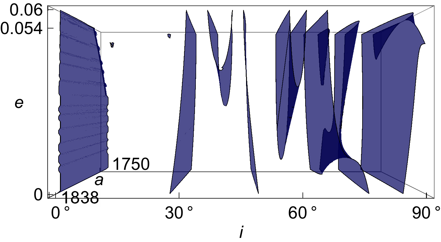
The plot shown in Fig. 1 can vary slightly for different values of semi-major axis within the range of low orbits. In order to illustrate that variation, Fig. 2 extends Fig. 1 by including a third axis that represents semi-major axis values from to km, thus corresponding to orbits with mean altitudes from to km. Red surfaces correspond to an argument of the periapsis of and blue surfaces to . As previously mentioned, only inclinations from to have been plotted, since inclinations between and show the same patterns for retrograde orbits.
3


With the aim of analyzing separately the effects of both the lunar gravitational field and the third-body attraction from the Earth over the families of frozen orbits, Fig. 3 includes a new plot with respect to Fig. 1, the red one, which represents the families of frozen orbits when the third-body effect is ignored. It is worth mentioning that this figure coincides with the central plot of Fig. 3 in Ref. [11]. As can be observed, the differences between the blue and the red plots are not significant for inclinations below approximately and their corresponding retrograde inclinations. Nevertheless, both plots exhibit important differences for frozen orbits near the polar region, for inclinations above and the equivalent retrograde orbits. In these cases, considering the gravitational pull from the Earth becomes indispensable, since it can make the difference between a feasible frozen orbit and a non-viable orbit with an eccentricity over the impact limit.
Finally, with the aim of highlighting the importance of considering the high-order harmonics of the lunar gravitational field for the purpose of searching for frozen orbits in real applications, we delve into the effect that each of the zonal harmonics contributes to the characterization of frozen orbits. A similar approach has been recently proposed in [28] to ascertain the correct truncation of the Geopotential required in orbit prediction problems. We plot separately the families of frozen orbits that correspond to the joint effect of the lunar gravitational field up to each individual order from to and the third-body attraction from the Earth. In general, every new harmonic that is included modifies very slightly the distribution of frozen orbits from lower-order terms. Nonetheless, there are three specific harmonics, , , and , that introduce variations in the number of families of frozen orbits. Then, in each of the graphics of Fig. 4 we gather together the plots that correspond to zonal consecutive harmonics with similar behavior, and include in blue the plot with the next harmonic that introduces a change in the number of families of frozen orbits. The same conventions from previous figures regarding the argument of the periapsis and the eccentricity limit for non-impact orbits also apply to Fig. 4.
2


Figure 4(a) shows a single critical inclination when only is considered. If is also included, Fig. 4(b), new frozen orbits appear with an argument of the periapsis of . The incorporation of the zonal harmonic in Fig. 4(c) implies that a new circular frozen orbit appears near the inclination of , whereas the one that already existed near is shifted towards a higher inclination, near . As a consequence of the former, a new family of frozen orbits appears for an argument of the periapsis of , whereas the latter implies that a wide region of inclinations between approximately and is deprived of feasible frozen orbits with eccentricities under the impact limit. In addition, the change in the argument of the periapsis that this circular frozen orbit caused before, from to , now becomes the opposite, that is, from to . Finally, Fig. 4(d) reveals a new family of frozen orbits surrounding the inclination of when is taken into account.
Higher-order harmonics over do not modify the number of families of frozen orbits, although they introduce variations in their evolution. In order to illustrate those changes, we divide the plots that correspond to the incorporation of every new harmonic into Figs. 5(a) and 5(b) for the sake of clarity, following the same conventions as in Fig. 4. The most important variations concern the feasibility of certain frozen orbits, which can cross the eccentricity limit for non-impact orbits in either direction when new harmonics are taken into account. That is especially significant for polar orbits, which, depending on the number of considered harmonics, can be frozen or not.
2


This analysis evinces the necessity of considering high-order lunar gravitational models when searching for low-altitude frozen orbits as part of a real mission-design process. Otherwise, certain families of frozen orbits will be missed, and the rest will be characterized with inaccurate values of eccentricity and inclination, especially in the region of polar orbits, to the extent that ignoring high-order harmonic coefficients can regard an impact orbit as a feasible frozen orbit. Therefore, it is essential to highlight that analyses that restrict their gravitational models to a few harmonics can only constitute academic studies, but can never be recommended for real applications.
4 Conclusion
We have conducted this study in order to clarify what the minimum resolution of the lunar gravitational potential should be considered when searching for frozen orbits in a real mission-design context, rather than within an academic scope. With this aim in view, we have developed a closed-form second-order semi-analytical theory for low-altitude orbiters around the Moon by applying perturbation methods based on Lie transforms. A lunar gravitational field has been considered, together with the third-body attraction from the Earth. The application of Lie transforms allows removing the short- and medium-period terms. Once an analytical theory is available, the full phase space of the dynamical system can be described, which allows, among other applications, characterizing the different families of frozen orbits. That can constitute a valuable tool for searching for frozen orbits in mission analysis and design, provided a reliable force model is used. In this study we have restricted the search for frozen orbits to the well-known argument-of-the-periapsis values of and . In principle, frozen orbits could also exist for other arguments of the periapsis, although, given the complexity of the expressions to manipulate, finding them can be a formidable task.
We have analyzed in depth the effect that changing the number of lunar harmonic coefficients that are considered produces on the distribution of families of frozen orbits. It has been verified that an insufficient order can miss certain families, and, what is worse, may predict the existence of valid frozen orbits at certain inclinations at which no frozen orbits exist for eccentricities below the impact limit. We have concluded that a gravitational model should be the minimum for real applications, thus confirming previous results in the scientific literature obtained with different techniques. Lower orders can only be regarded as academic studies, whereas in the case of higher orders, since the qualitative behavior no longer changes, the small gain in accuracy does not justify the significant increase in the computational load.
Likewise, the influence of the gravitational attraction from the Earth has also been analyzed. It can be concluded that the effect of this perturbation on the distribution of families of frozen orbits is especially important for orbits near the polar region, at inclinations above approximately , where this third-body effect allows for the existence of viable frozen orbits that, otherwise, would not be possible for eccentricities below the impact limit.
Finally, we have implemented this semi-analytical theory in a Mathematica package for mission planning, which allows finding suitable frozen conditions that constitute an accurate first approximation for a periodic orbit in the original space, once mean elements have been converted into osculating elements, that is, once the short- and medium-period terms have been recovered.
Funding Sources
This work has been funded by the Spanish State Research Agency and the European Regional Development Fund under Project ESP2016-76585-R (AEI/ERDF, EU).
Acknowledgments
The authors would like to thank two anonymous reviewers for their valuable suggestions.
References
- Coffey et al. [1994] Coffey, S. L., Deprit, A., and Deprit, E., “Frozen orbits for satellites close to an Earth-like planet,” Celestial Mechanics and Dynamical Astronomy, Vol. 59, No. 1, 1994, pp. 37–72. 10.1007/BF00691970.
- Cook [1966] Cook, G. E., “Perturbations of near-circular orbits by the Earth’s gravitational potential,” Planetary and Space Science, Vol. 14, No. 5, 1966, pp. 433–444. 10.1016/0032-0633(66)90015-8.
- Rosborough and Ocampo [1992] Rosborough, G. W., and Ocampo, C. A., “Influence of higher degree zonals on the frozen orbit geometry,” Advances in the Astronautical Sciences, Vol. 76, 1992, pp. 1291–1304. Paper AAS 91-428.
- Kiedron and Cook [1992] Kiedron, K., and Cook, R., “Frozen orbits in the problem,” Advances in the Astronautical Sciences, Vol. 76, 1992, pp. 1273–1289. Paper AAS 91-426.
- Cook [1992] Cook, R. A., “The long-term behavior of near-circular orbits in a zonal gravity field,” Advances in the Astronautical Sciences, Vol. 76, 1992, pp. 2205–2221. Paper AAS 91-463.
- Folta et al. [1998] Folta, D., Galal, K., and Lozier, D., “Lunar prospector frozen orbit mission design,” Proceedings 1998 AIAA/AAS Astrodynamics Specialist Conference and Exhibit, American Institute of Aeronautics and Astronautics, Boston, MA, USA, 1998. 10.2514/6.1998-4288, paper AIAA-98-4288.
- Park and Junkins [1994] Park, S. Y., and Junkins, J. L., “Orbital mission analysis for a lunar mapping satellite,” Proceedings 1994 AIAA/AAS Astrodynamics Conference, American Institute of Aeronautics and Astronautics, Scottsdale, AZ, USA, 1994, pp. 93–98. 10.2514/6.1994-3717, paper AIAA-94-3717-CP.
- Folta and Quinn [2006] Folta, D., and Quinn, D., “Lunar frozen orbits,” Proceedings 2006 AIAA/AAS Astrodynamics Specialist Conference and Exhibit, American Institute of Aeronautics and Astronautics, Keystone, CO, USA, 2006. 10.2514/6.2006-6749, paper AIAA 2006-6749.
- Kozai [1963] Kozai, Y., “Motion of a lunar orbiter,” Publications of the Astronomical Society of Japan, Vol. 15, No. 3, 1963, pp. 301–312.
- Lara et al. [2009] Lara, M., Ferrer, S., and De Saedeleer, B., “Lunar analytical theory for polar orbits in a 50-degree zonal model plus third-body effect,” The Journal of the Astronautical Sciences, Vol. 57, No. 3, 2009, pp. 561–577. 10.1007/BF03321517.
- Lara [2011] Lara, M., “Design of long-lifetime lunar orbits: a hybrid approach,” Acta Astronautica, Vol. 69, No. 3-4, 2011, pp. 186–199. 10.1016/j.actaastro.2011.03.009.
- Russell and Lara [2007] Russell, R. P., and Lara, M., “Long-lifetime lunar repeat ground track orbits,” Journal of Guidance, Control, and Dynamics, Vol. 30, No. 4, 2007, pp. 982–993. 10.2514/1.27104.
- Roncoli [2005] Roncoli, R. B., “Lunar constants and models document,” Tech. Rep. JPL D-32296, Jet Propulsion Laboratory, California Institute of Technology, Pasadena, CA, USA, September 2005.
- San-Juan et al. [2008] San-Juan, J. F., Abad, A., Elipe, A., and Tresaco, E., “Analytical model for lunar orbiter,” Advances in the Astronautical Sciences, Vol. 130, 2008, pp. 1281–1299. Paper AAS 08-184.
- San-Juan [2010] San-Juan, J. F., “Analytical model for lunar orbiter revisited,” Advances in the Astronautical Sciences, Vol. 136, 2010, pp. 245–263. Paper AAS 10-116.
- Abad et al. [2009] Abad, A., Elipe, A., and Tresaco, E., “Analytical model to find frozen orbits for a lunar orbiter,” Journal of Guidance, Control, and Dynamics, Vol. 32, No. 3, 2009, pp. 888–898. 10.2514/1.38350.
- Konopliv et al. [1994] Konopliv, A. S., Sjogren, W. L., Wimberly, R. N., Cook, R. A., and Vijayaraghavan, A., “A high resolution lunar gravity field and predicted orbit behavior,” Advances in the Astronautical Sciences, Vol. 85, 1994, pp. 1275–1294. Paper AAS 93-622.
- Garfinkel [1965] Garfinkel, B., “Tesseral harmonic perturbations of an artificial satellite,” The Astronomical Journal, Vol. 70, No. 10, 1965, pp. 784–786. 10.1086/109817.
- Deprit [1981] Deprit, A., “The elimination of the parallax in satellite theory,” Celestial Mechanics, Vol. 24, No. 2, 1981, pp. 111–153. 10.1007/BF01229192.
- San-Juan et al. [2013] San-Juan, J. F., Ortigosa, D., López-Ochoa, L. M., and López, R., “Deprit’s elimination of the parallax revisited,” The Journal of the Astronautical Sciences, Vol. 60, No. 2, 2013, pp. 137–148. 10.1007/s40295-015-0033-5.
- Lara et al. [2014] Lara, M., San-Juan, J. F., and López-Ochoa, L. M., “Proper averaging via parallax elimination,” Advances in the Astronautical Sciences, Vol. 150, 2014, pp. 315–331. Paper AAS 13-722.
- Deprit [1982] Deprit, A., “Delaunay normalisations,” Celestial Mechanics, Vol. 26, No. 1, 1982, pp. 9–21. 10.1007/BF01233178.
- San-Juan et al. [2015] San-Juan, J. F., López, R., Pérez, I., and San-Martín, M., “A note about certain arbitrariness in the solution of the homological equation in Deprit’s method,” Mathematical Problems in Engineering, Vol. 2015, 2015, p. 10 pages. 10.1155/2015/982857, article ID 982857.
- San-Juan et al. [2011] San-Juan, J. F., López, L. M., and López, R., “MathATESAT: A symbolic-numeric environment in Astrodynamics and Celestial Mechanics,” Lecture Notes in Computer Science, Vol. 6783, No. 2, 2011, pp. 436–449. 10.1007/978-3-642-21887-3_34.
- Coffey et al. [1986] Coffey, S. L., Deprit, A., and Miller, B. R., “The critical inclination in artificial satellite theory,” Celestial Mechanics, Vol. 39, No. 4, 1986, pp. 365–406. 10.1007/BF01230483.
- Coffey et al. [1990] Coffey, S., Deprit, A., Deprit, E., and Healy, L., “Painting the phase space portrait of an integrable dynamical system,” Science, Vol. 247, No. 4944, 1990, pp. 833–836. 10.1126/science.247.4944.833.
- Ferrer et al. [2007] Ferrer, S., San-Juan, J. F., and Abad, A., “A note on lower bounds for relative equilibria in the main problem of artificial satellite theory,” Celestial Mechanics and Dynamical Astronomy, Vol. 99, No. 1, 2007, pp. 69–83. 10.1007/s10569-007-9091-8.
- Lara [2018] Lara, M., “Exploring sensitivity of orbital dynamics with respect to model truncation: the frozen orbits approach,” Stardust Final Conference - Advances in Asteroids and Space Debris Engineering and Science, Astrophysics and Space Science Proceedings, Vol. 52, edited by M. Vasile, E. Minisci, L. Summerer, and P. McGinty, Springer International Publishing, Cham, Switzerland, 2018, pp. 69–83. 10.1007/978-3-319-69956-1_4.
- Konopliv et al. [2001] Konopliv, A. S., Asmar, S. W., Carranza, E., Sjogren, W. L., and Yuan, D. N., “Recent gravity models as a result of the Lunar Prospector mission,” Icarus, Vol. 150, No. 1, 2001, pp. 1–18. 10.1006/icar.2000.6573.
- Matsumoto et al. [2010] Matsumoto, K., Goossens, S., Ishihara, Y., Liu, Q., Kikuchi, F., Iwata, T., Namiki, N., Noda, H., Hanada, H., Kawano, N., Lemoine, F. G., and Rowlands, D. D., “An improved lunar gravity field model from SELENE and historical tracking data: revealing the farside gravity features,” Journal of Geophysical Research, Planets, Vol. 115, No. E6, 2010, pp. 1–20. 10.1029/2009JE003499.
- Mazarico et al. [2010] Mazarico, E., Lemoine, F. G., Han, S. C., and Smith, D. E., “GLGM-3: a degree-150 lunar gravity model from the historical tracking data of NASA Moon orbiters,” Journal of Geophysical Research, Planets, Vol. 115, No. E5, 2010, pp. 1–14. 10.1029/2009JE003472.
- Konopliv et al. [2013] Konopliv, A. S., Park, R. S., Yuan, D. N., Asmar, S. W., Watkins, M. M., Williams, J. G., Fahnestock, E., Kruizinga, G., Paik, M., Strekalov, D., Harvey, N., Smith, D. E., and Zuber, M. T., “The JPL lunar gravity field to spherical harmonic degree 660 from the GRAIL Primary Mission,” Journal of Geophysical Research, Planets, Vol. 118, No. 7, 2013, pp. 1415–1434. 10.1002/jgre.20097.