HIGH-FIDELITY DIGITAL TWINS: DETECTING AND LOCALIZING WEAKNESSES IN STRUCTURES
Abstract.
An adjoint-based procedure to determine weaknesses, or, more generally,
the material properties of structures is developed and tested. Given a
series of load cases and corresponding displacement/strain
measurements, the material
properties are obtained by minimizing the weighted differences
between the measured and computed values. In a subsequent step,
techniques to minimize the number of load cases and sensors are
proposed and tested.
Several examples show the viability, accuracy and efficiency of
the proposed methodology and its potential use for
high fidelity digital twins.
1. Introduction
Given that all materials exposed to the environment and/or undergoing
loads eventually age and fail, the task of trying to detect and localize
weaknesses in structures is common to many fields. To mention just a few:
airplanes, drones, turbines, launch pads and airport
and marine infrastructure, bridges, high-rise buildings, wind turbines,
and satellites.
Traditionally, manual inspection was the only way of carrying out this task,
aided by ultrasound, X-ray, or vibration analysis techniques.
The advent of accurate, abundant and cheap sensors, together with
detailed, high-fidelity computational models
in an environment of digital twins has opened the possibility of
enhancing and automating the detection and localization of
weaknesses in structures.
From an abstract setting, it would seem that the task of determining
material properties from loads and measurements is an ill-posed
problem. After all, if we think of atoms, granules or some polygonal
(e.g. finite element [FEM]) subdivision of space, the amount of data
given resides in a much smaller space than the data sought.
If we think of a cuboid domain in dimensions with subdivisions,
the maximum amount of surface information/ data given is of
while the data sought is of .
Another aspect that would seem to imply that this is an ill-posed
problem is the possibility that many different spatial distributions
of material properties could yield very similar or equal displacements
under loads.
On the other hand, the propagation of physical properties (e.g.
displacements, temperature, electrical currents, etc.) through the
domain obeys physical conservation laws, i.e. some partial differential
equations (PDEs). This implies that the material properties that can give
rise to the data measured on the boundary are restricted by these
conservation laws, i.e. are constrained. This would indicate that perhaps
the problem is not as ill-posed as initially thought.
As the task of damage detection is of such importance, many
analytical techniques have been developed over the last decades
[7, 13, 18, 12, 23, 22, 21, 8, 20, 2, 5, 11].
Some of these were developed to identify weaknesses in
structures, others (e.g. [13]) to
correct or update finite element models.
The damage/weakness detection from measurements falls into
the more general class of inverse problems where material properties
are sought based on a desired cost functional
[4, 14, 6, 24]. It is known that these inverse
problems are ill-defined and require regularization techniques.
The analytical methods depend on the measurement device
at hand, and one can classify broadly according to them.
The first class of analytical methods is based on changes
observed in (steady) displacements or strains
[22, 8, 2, 25, 11]. The second
class considers velocities or accelerations in the time domain
[12, 23, 20].
The third class is based on changes observed in the frequency domain
[7, 13, 18, 21, 6].
Some of the methods based on displacements, strains, velocities or
accelerations used adjoint formulations
[27, 22, 8, 20, 3, 25, 17]
in order to obtain the gradient of the cost function with the least
amount of effort. In the present case, the procedures used are
also based on measured forces and displacements/strains, use adjoint
formulations and smoothing of gradients to quickly localize damaged
regions [1]. Unlike previous efforts, they are intended for
weakness/damage detection in the context of digital twins, i.e. we
assume a set of defined loadings
and sensors that accompany the structure (object, product, process)
throughout its lifetime in order to monitor its state. The digital
twins are assumed to contain finite element discretizations/models
of high fidelity, something that nowadays is common the aerospace
industry. Therefore, the proposed approach fits well into the overall
workflow of high-level CAD environments and high fidelity FEM models
seen in the design phase.
2. Assumptions
What follows relies on the following set of assumptions:
-
-
Monitoring the weakening of a structure is carried out by applying a set of different forces and measuring the resulting displacements and/or strains at different locations (the intrinsic assumption is that the forces can be standardized and perhaps even maintained throughout the life of the structure);
-
-
The weakening of a structure may occur at any location, i.e. there are no regions that are excluded for weakening; this is the most conservative assumption, and could be relaxed under certain conditions;
-
-
The sensors for displacements and strains are limited in their ability to measure by noise/signal ratios, i.e. actual displacements and strains have to be larger than a certain threshold to be of use:
(2.1) -
-
The type of force used to monitor the weakening of a structure is limited by practical considerations; this implies that the number of different forces is limited, and can not assume arbitrary distributions in space.
-
-
The weakening of a structure may be described by a field , where and corresponds to total failure (no load bearing capability) while is the original state;
- -
-
where are the displacements and the usual stiffness matrix, which is obtained by assembling all the element matrices:
(2.3)
3. Determining material properties via optimization
The determination of material properties (or weaknesses) may be formulated as an optimization problem for the strength factor as follows: Given force loadings and corresponding measurements at measuring points/locations of their respective displacements or strains , obtain the spatial distribution of the strength factor that minimizes the cost function:
| (3.1) |
subject to the finite element description (e.g. trusses, beams, plates, shells, solids) of the structure [28, 26] under consideration (i.e. the digital twin/system [18, 9]):
| (3.2) |
where are displacement and strain weights, interpolation matrices that are used to obtain the displacements and strains from the finite element mesh at the measurement locations, and the usual stiffness matrix, which is obtained by assembling all the element matrices:
| (3.3) |
where the strength factor of the elements has already been incorporated. We note in passing that in order to ensure that is invertible and non-degenerate . Note that the optimization problem given by Eqns.(3.1)-(3.3) does not assume any specific choice of finite element basis functions, i.e. is widely applicable.
3.1. Optimization via adjoints
The objective function can be extended to the Lagrangian functional
| (3.4) |
where are the Lagrange multipliers (adjoints). Variation of the Lagrangian with respect to each of the measurements then results in:
| (3.5a) | |||
| (3.5b) | |||
| (3.5c) | |||
where denotes the relationship between the displacements
and strains (i.e. the derivatives of the displacement field on the
finite element mesh and the location (see Section 4 below)).
The consequences of this rearrangement are profound:
-
-
The gradient of , with respect to may be obtained by solving forward and adjoint problems; i.e.
-
-
Unlike finite difference methods, which require at least forward problems per design variable, the number of forward and adjoint problems to be solved is independent of the number of variables used for (!);
-
-
Once the forward and adjoint problems have been solved, the cost for the evaluation of the gradient of each design variable only involves the degrees of freedom of the element, i.e. is of complexity ;
-
-
For most structural problems , so if a direct solver has been employed for the forward problem, the cost for the evaluation of the adjoint problems is negligible;
-
-
For most structural problems , so if an iterative solver is employed for the forward and adjoint problems, the preconditioner can be re-utilized.
3.2. Optimization steps
An optimization cycle using the adjoint approach is composed
of the following steps:
For each force/measurement pair :
-
-
With current : solve for the displacements
-
-
With current , and : solve for the adjoints
-
-
With : obtain gradients
Once all the gradients have been obtained:
-
-
Sum up the gradients
-
-
If necessary: smooth gradients
-
-
Update .
Here is a small stepsize that can be adjusted so as to obtain optimal convergence (e.g. via a line search method).
4. Interpolation of displacements and strains
The location of a displacement or strain gauge may not coincide with any of the nodes of the finite element mesh. Therefore, in general, the displacement at a measurement location needs to be obtained via the interpolation matrix as follows:
| (4.1) |
where are the values of the displacements vector at all
gridpoints.
In many cases it is much simpler to install strain gauges instead of
displacement gauges. In this case, the strains need to be obtained
from the displacement field. This can be written formally as:
| (4.2) |
where the ‘derivative matrix’ contains the local values of the derivatives of the shape-functions of . The strain at an arbitrary position is obtained via the interpolation matrix as follows:
| (4.3) |
Note that in many cases the strains will only be defined in the elements, so that the interpolation matrices for displacements and strains may differ.
5. Choice of weights
The cost function is given by Eqn.(3.1), repeated here for clarity:
| (5.1) |
One can immediately see that the dimensions of displacements and strains are different. This implies that the weights should be chosen in order that all the dimensions coincide. The simplest way of achieving this is by making the cost function dimensionless. This implies that the displacement weights should be of dimension [1/(displacement*displacement)] (the strains are already dimensionless). Furthermore, in order to make the procedures more generally applicable they should not depend on a particular choice of measurement units (metric, imperial, etc.). This implies that the weights for the displacements and strains should be of the order of the characteristic or measured magnitude. Several options are possible, listed below.
5.1. Local Weighting
In this case
| (5.2) |
this works well, but may lead to an ‘over-emphasis’ of small displacements/strains that are in regions of marginal interest.
5.2. Average weighting
In this case one first obtains the average of the absolute value of the displacements/strains for a loadcase and uses them for the weights, i.e.:
| (5.3) |
this works well, but may lead to an ‘under-emphasis’ of small displacements/strains that may occur in important regions.
5.3. Max weighting
In this case one first obtains the maximum of the absolute value of the displacements/strains for a loadcase and uses them for the weights, i.e.:
| (5.4a) | |||
| (5.4b) | |||
this also works well for many cases, but may lead to an ‘under-emphasis’ of smaller displacements/strains that can occur in important regions.
5.4. Local/Max weighting
In this case
| (5.5) |
with ; this seemed to work best of all, as it combines local weighting with a max-bound minimum for local values.
6. Smoothing of gradients
The gradients of the cost function with respect to allow for oscillatory solutions. One must therefore smooth or ‘regularize’ the spatial distribution. This happens naturally when using few degrees of freedom, i.e. when is defined via other spatial shape functions (e.g. larger spatial regions of piecewise constant [22]). As the (possibly oscillatory) gradients obtained in the (many) finite elements are averaged over spatial regions, an intrinsic smoothing occurs. This is not the case if and the gradient are defined and evaluated in each element separately, allowing for the largest degrees of freedom in a mesh and hence the most accurate representation. Three different types of smoothing or ‘regularization’ were considered. All of them start by performing a volume averaging from elements to points:
| (6.1) |
where denote the value of at point , as well as the values of in element and the volume of element , and the sum extends over all the elements surrounding point .
6.1. Simple point/element/point averaging
In this case, the values of are cycled between elements and points. When going from point values to element values, a simple average is taken:
| (6.2) |
where denotes the number of nodes of an element and the sum extends over all the nodes of the element. After obtaining the new element values via Eqn.(6.2) the point averages are again evaluated via Eqn.(6.1). This process is repeated for a specified number of iterations (typically 1-5). While very crude, this form of averaging works surprisingly well.
6.2. (Weak) Laplacian Smoothing
In this case, the initial values obtained for are smoothed via:
| (6.3) |
Here is a free parameter which may be problem and mesh dependent (its dimensional value is length squared). Discretization via finite elements yields:
| (6.4) |
where denote the consistent mass matrix, the stiffness or ‘diffusion’ matrix obtained for the Laplacian operator and the projection matrix from element values () to point values ().
6.3. Pseudo-Laplacian Smoothing
One can avoid the dimensional dependency of by smoothing via:
| (6.5) |
where is a characteristic element size. For linear elements, one can show that this is equivalent to:
| (6.6) |
where denotes the lumped mass matrix [15]. In the examples shown below this form of smoothing was used for the gradients, setting .
7. Implementation in black-box solvers
The optimization cycle outlined above can be implemented in a very efficient way if one has direct access to the source-code of finite element-based structural mechanics solvers, but is also amenable to black-box (e.g. commercial) solvers. A possible way to proceed is the following:
-
-
Output the original stiffness matrix for each element;
-
-
For each optimization step/cycle:
-
-
With the current element values for : build the new stiffness matrix; this is usually done with a user-defined subroutine or module (all commercial codes allow for that);
-
-
For each load case :
-
-
Solve the forward problem ();
-
-
Post-process the results of the forward problem in order to obtain the displacements and strains;
-
-
With the measured and computed displacements/ strains and weights: compute the cost function part of this load case ();
-
-
Build the ‘force vector’ (i.e. the right-hand-side) for the adjoint problem by comparing the measured and computed displacements/ strains and weighting them appropriately;
-
-
Solve the adjoint problem ();
-
-
With and the original stiffness matrix : get the gradient in each element;
-
-
Smooth the gradients (either via a ‘fake-heat-solver’ if Laplacian smoothing is desired, or via an external smoother);
-
-
Send the cost function and the smoothed gradients to the optimizer;
-
-
Update
8. Optimization of loadings
The aim of choosing a minimal yet optimal set of forces to monitor
the weakening of structures is to be able to determine the
field as best as possible. From structural mechanics,
this implies that one should avoid regions where the strains are very
small or vanish. For these regions, can assume an
arbitrary value without having any effect on the overall displacements
or strains. Therefore, the forces should be chosen such that the
number of regions with very small or vanishing strains should be
minimized.
As stated before, for practical reasons the number and type of possible
loads is limited. This ‘limitation of the search space for loads’ opens
up the possibility of a simple algorithm to determine the optimal
choice. For each of the possible loads ,
obtain the resulting displacement and strains, and record all
elements for which the strains are above a minimal sensor
threshold .
If only one force is to be applied, the obvious choice is to select
the one that produces the largest area with strains that are above
a minimal threshold. Having selected this force, the regions
that have already been affected by this force (i.e. with strains
that are above the minimal threshold) are excluded
from further consideration. The next best force is then again the one that
is able to measure the largest area with strains that are above
a minimal threshold. And so on recursively.
9. Optimal placement of sensors
Let us assume that a certain part of the structure has weakened. This could be a region of several elements, or a single element. This will lead to a change in the stiffness matrix, and a resulting change in displacements and strains. The aim is to be able to record and identify the spatial location of this weakening with the minimum number of sensors. The change in displacements or strains due to a weakening requires the evaluation of the derivative
| (9.1) |
for all possible combination of locations .
In the most general case is arbitrary, i.e. it could
be any node or element of the mesh. However, if sensors can only
be placed in certain regions of the domain, the location of
can be reduced significantly.
Two possible ways were explored to obtain :
forward-based and adjoint-based.
9.1. Forward-based
An immediate approach takes each ‘region of elements’, changes the stiffness matrix and computes the resulting changes in displacements and strains at the possible sensor locations. Dropping the index for the load cases, for each of them this results in:
| (9.2) |
With the original system (Eqn.(2.2)) this results in:
| (9.3) |
As the inverse (or LU decomposed) matrix of is assumed as
given (it was needed to compute ), there are now two options:
a) Neglect the higher order terms ,
which results in:
| (9.4) |
b) Iterate for :
| (9.5) |
One is now able to determine for each possible weakening region
the resulting deformations and strains, and
with the thresholds those sensors that are able to
monitor the weakening.
The effect of weakening a region (in the
extreme case a single element) on the sensors implies, in the
worst case, a CPU requirement that is of order
for each of the load
cases, where denotes the
number of elements and the bandwidth of the system
matrix . Clearly, for large problems with
this can become costly. Several options to manage this high cost
are treated in Section 9.4.
9.2. Adjoint-based
A more elegant (and faster) approach makes use of the adjoint to obtain the desired sensitivities for each possible sensor locations. The desired quantity whose derivative with respect to element strength factor is sought (e.g. displacement at a sensor location) can be written as:
| (9.6) |
The desired derivative is given by:
| (9.7) |
This can be augmented to a Lagrangian by invoking the elasticity equations, resulting in:
| (9.8) |
The derivatives result in the usual systems of equations:
| (9.9a) | |||
| (9.9b) | |||
| (9.9c) | |||
Using the adjoint the information sought is evaluated in
the opposite order to the previous (forward, element-based)
procedure. While in the forward case an element/region was weakened
resulting in displacements/strains for all nodes/elements, in the
adjoint case a location is selected and the effect of weakening
each element on this location is obtained.
Observe that in this case the CPU requirement is of order
for each of the
loadcases, where denotes the number of sensors (assumed to be
much lower than the number of elements), the number of
elements and the bandwidth of the system matrix .
The advantages of using the adjoint may become even more pronounced
for nonlinear problems. While the forward-based procedure would
require the solution of a nonlinear problem for each element
(or element group), the adjoint always remains a linear problem.
9.3. Sensor placement
If only one sensor is to be placed, the obvious choice is to select the one that is able to measure the highest number of weakening regions. Having selected this sensor, the weakening regions that were able to be measured are excluded from further consideration. The next best sensor is then again the one that is able to measure the highest number of the remaining weakening regions. And so on recursively.
9.4. Implementation details
There are two aspects of the sensitivity calculation procedures for optimal sensor placement that need to be addressed: computation and storage requirements.
9.5. Computation
The effect of weakening a region (in the extreme case a single element) for the forward option, or the sensitivity of each element/point in the mesh for the adjoint option implies, in the worst case, a CPU requirement that is of order , where denotes the number of elements and the bandwidth of the system matrix . Clearly, for large problems with this can become costly. As is so often the case in computational mechanics, algorithms and hardware can help alleviate this problem.
Clustering of elements
Instead of weakening a single element (forward option) or computing the sensity of a single node/element (adjoint option), one can cluster elements into subregions. The CPU requirements then decrease to , where denotes the number of subregions. In the present case an advancing front technique was used to cluster elements into subregions. The size of the subregions can be specified via a minimum required number of elements per subregion, the area/volume of the subregion or the minimum distance from the first element/point of the subregion. Given that in 3-D the number of elements in a subregion increases quickly, the number of subregions can be substantially lower than the number of elements, yielding a considerable reduction in CPU requirements.
Parallel computing
The matrix problem that needs to be solved to obtain the effect of weakening a region/element (forward option) or to obtain the sensitivity of a region/element (adjoint option) is independent of other regions/elements, making the problem embarrassingly parallel.
9.6. Storage
Storing the effect of weakening a region (in the extreme case a single element) or the sensitivity of all elements for every element implies, in the worst case, a storage requirement that is of order . Even if one is only interested in the effect on sensors this implies . Clearly, for large problems with and this can become an issue. A simple way to diminish the storage requirements is to store the on/off sensing in powers of 2:
| (9.10) |
where is either or depending on whether the sensor was activated or not.
9.7. Sensor placement with regions
In some cases, the weakening of all elements can be achieved with only a few sensors (in the extreme case a single sensor). However, placing a single sensor would preclude being able to precisely define weakening regions. Therefore, only the elements in the neighbourhood of the selected sensor are excluded from further consideration. As before, the neighbourhood of the sensor can be specified via the number of elements, the area/volume or the distance from the sensor. The remainder of the procedure outlined above remains the same.
10. Examples
All the numerical examples were carried out using two finite element codes. The first, FEELAST [16], is a finite element code based on simple linear (truss), triangular (plate) and tetrahedral (volume) elements with constant material properties per element that only solves the linear elasticity equations. The second, CALCULIX [10], is a general, open source finite element code for structural mechanical applications with many element types, material models and options. The optimization loops were steered via a simple shell-script for the adjoint-based gradient descent method. In all cases, a ‘target’ distribution of was given, together with defined external forces . The problem was then solved, i.e. the displacements and strains were obtained and recorded at the ‘measurement locations’ . This then yielded the ‘measurement pair’ or that was used to determine the material strength distributions in the field.
10.1. Plate with hole
The case is shown in Figures 10.1 and 10.2, and considers a plate with a hole. The plate dimensions are (all units in cgs): , , . A hole of diameter is placed in the middle (). Density, Young’s modulus and Poisson rate were set to respectively. 672 linear, triangular, plain stress elements were used. The left boundary of the plate is assumed clamped (), while a horizontal load of was prescribed at the right end. In the first instance, a small region of weakened material was specified. The ability of the procedure to detect or ‘recover’ this weakening based on the number of sensors used (shown as white dots) is clearly visible. As the number of sensors increases, the region is recovered. Notice that even with 1 sensor a weakening is already detected, and that with 6 sensors the weakened region is clearly defined.
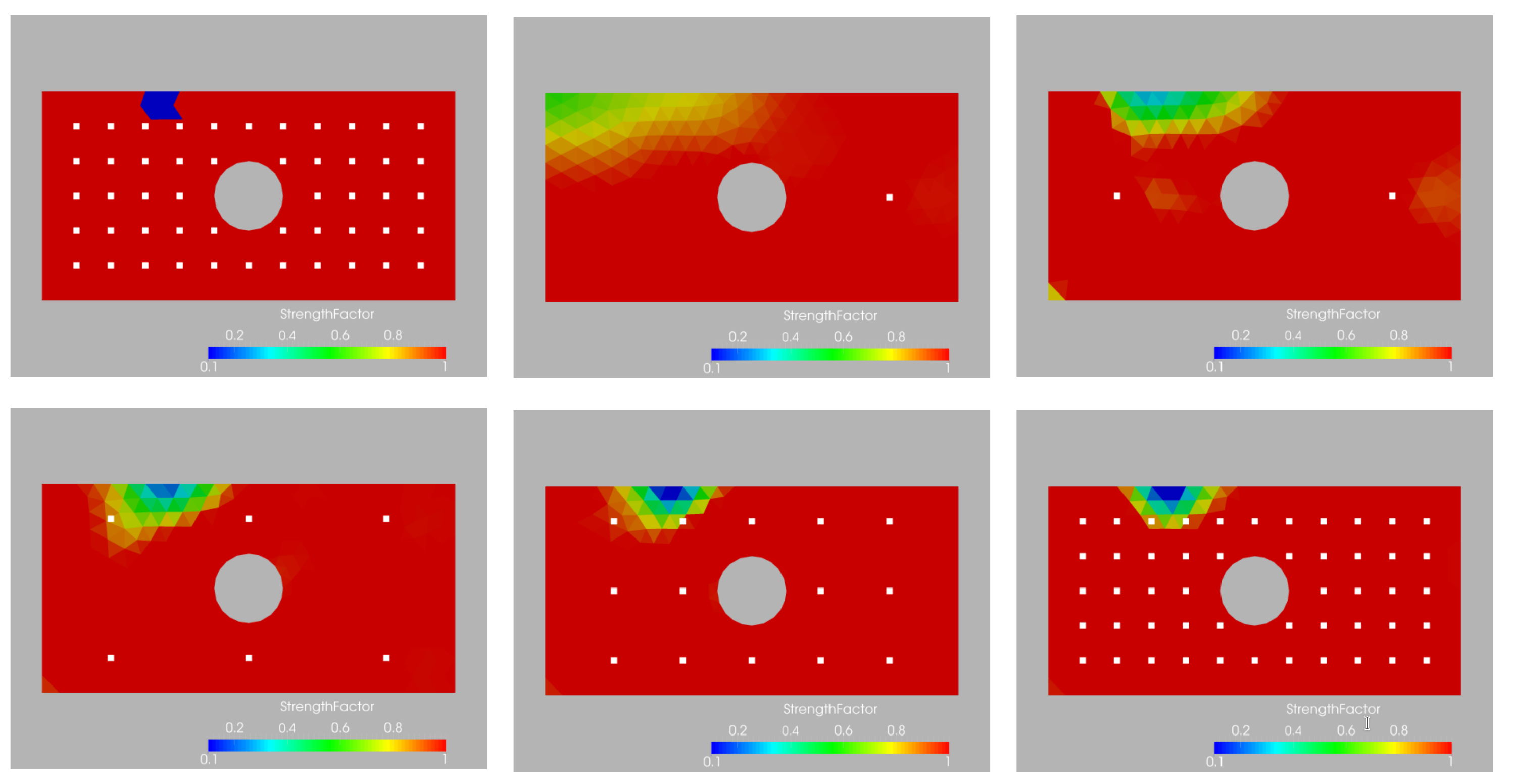
In the second case, four weakening regions were specified.
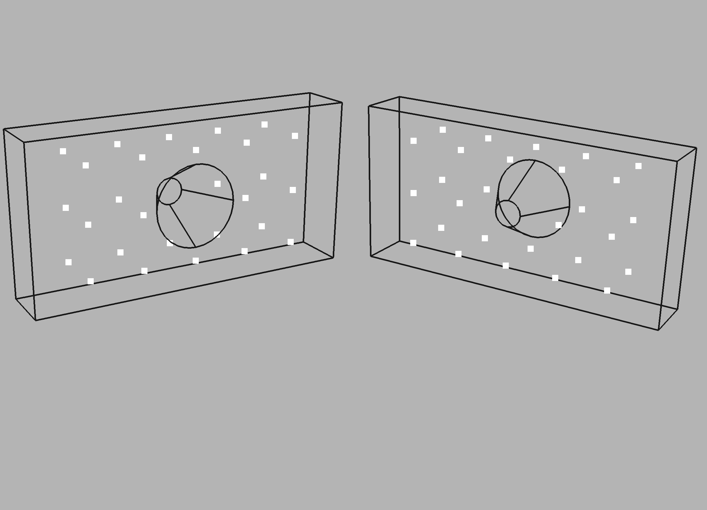
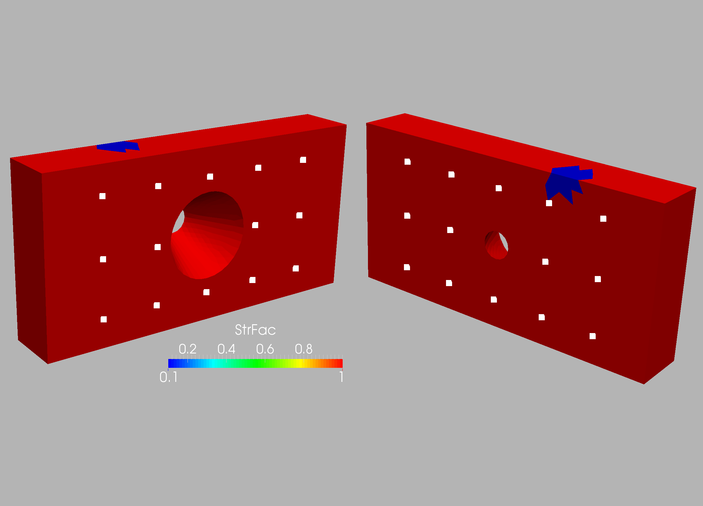
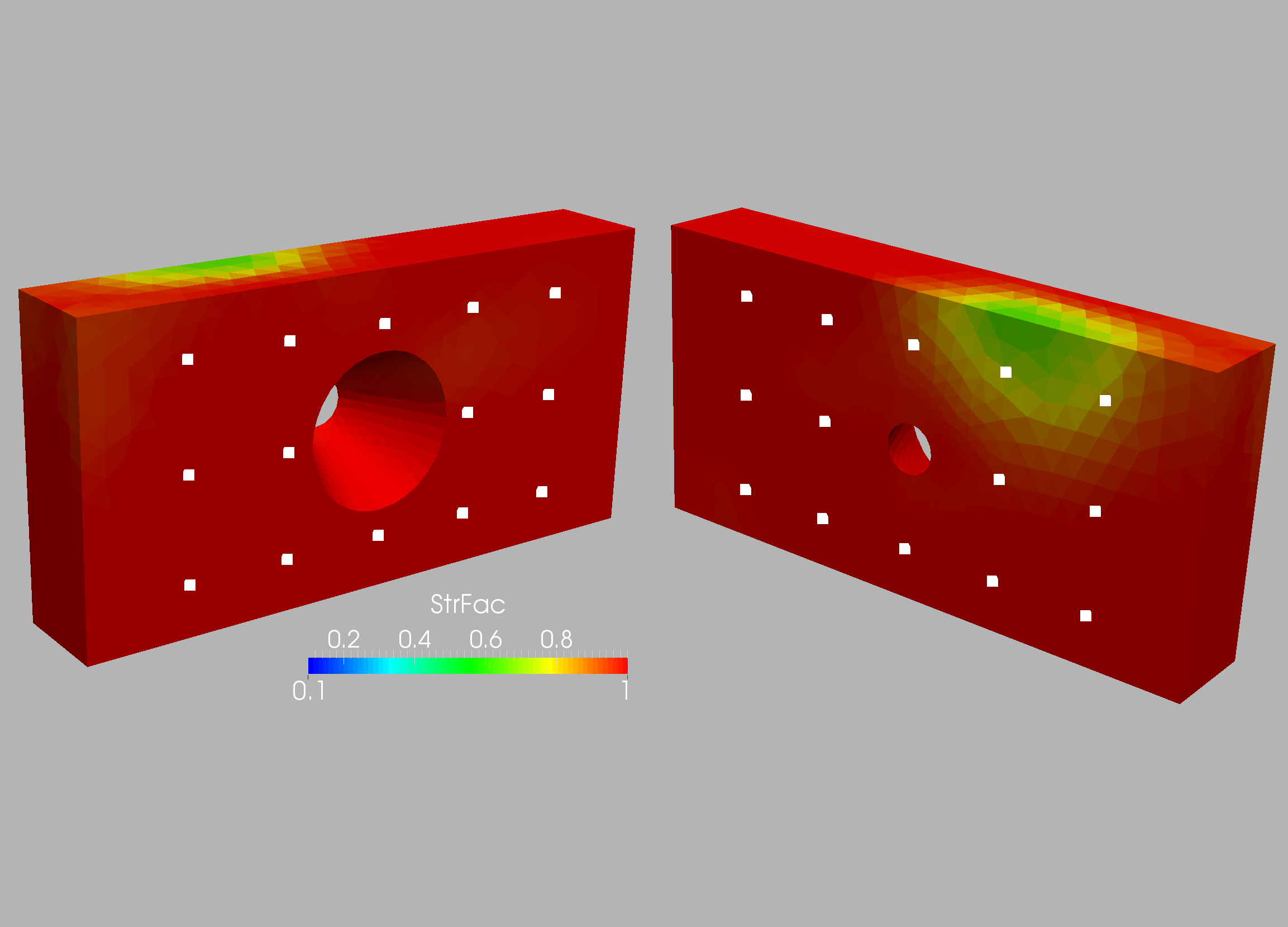
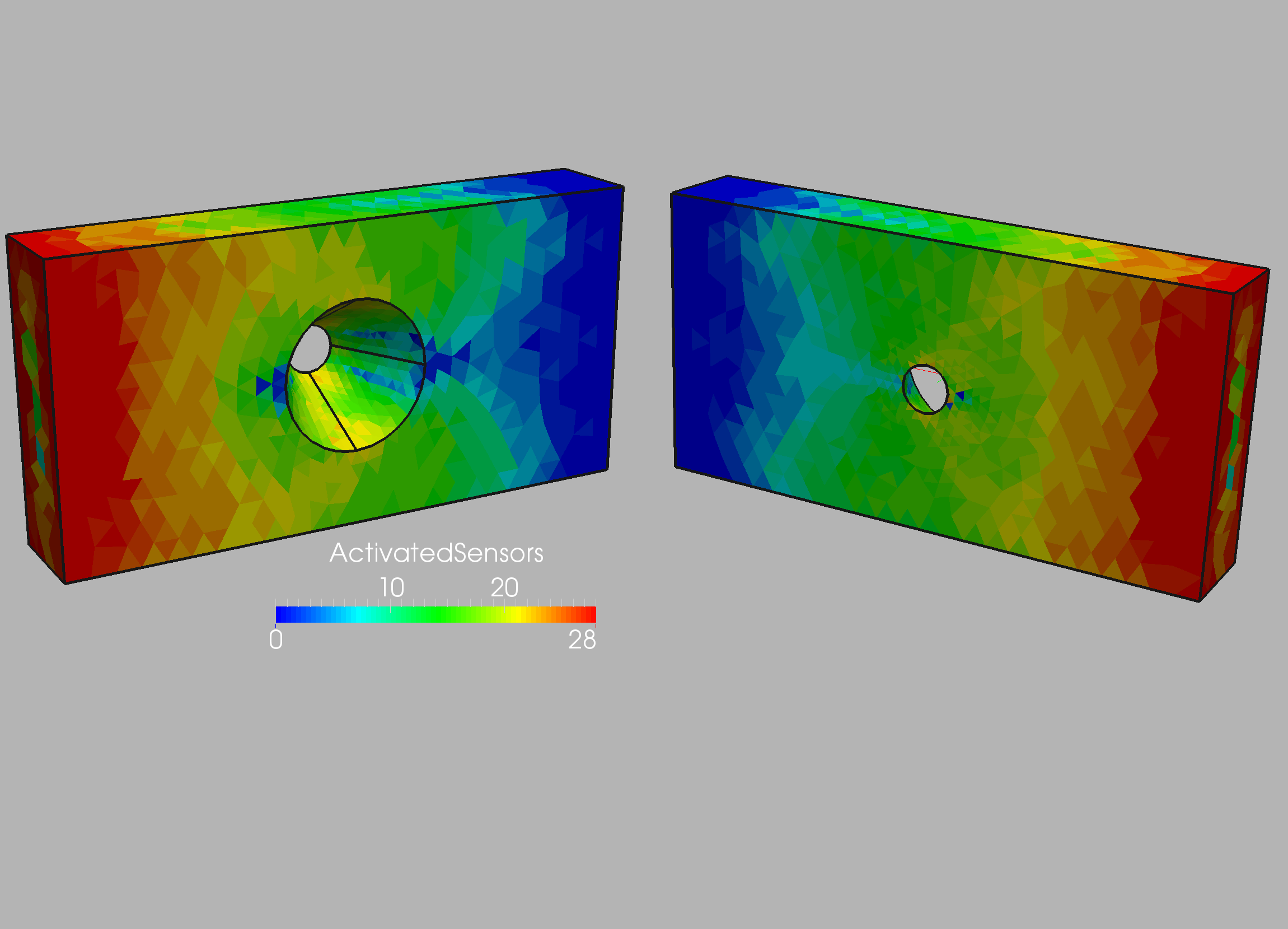
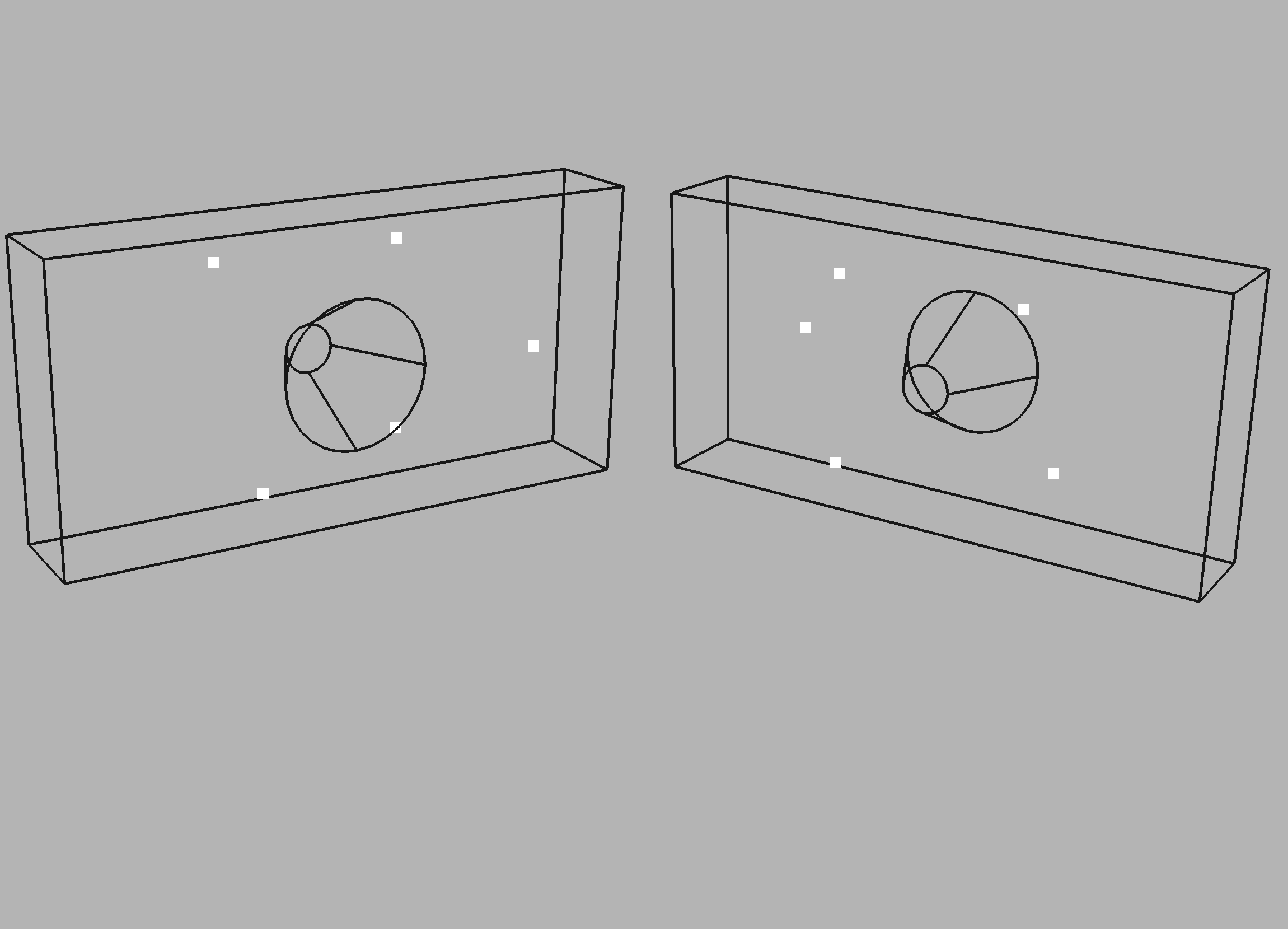
10.2. Thick plate with conical hole
The case is shown in Figure 10.3 and considers a thick plate
with a conical hole. The plate dimensions are (all units in cgs):
, , . A conical hole
of diameter and is placed in the middle ().
Density, Young’s modulus and Poisson rate were set to
respectively.
Two grids, of 19 K and 120 K linear tetrahedral elements (tet) were
used. The surface mesh of the coarser mesh
is shown in Figure 10.3. A first series of runs with the 28 sensors
shown in Figure 10.4 were conducted. The target and computed weakening
for the two grids and the 28 sensors are shown in Figures 10.5-10.8.
Note the proper detection of the weakened region.
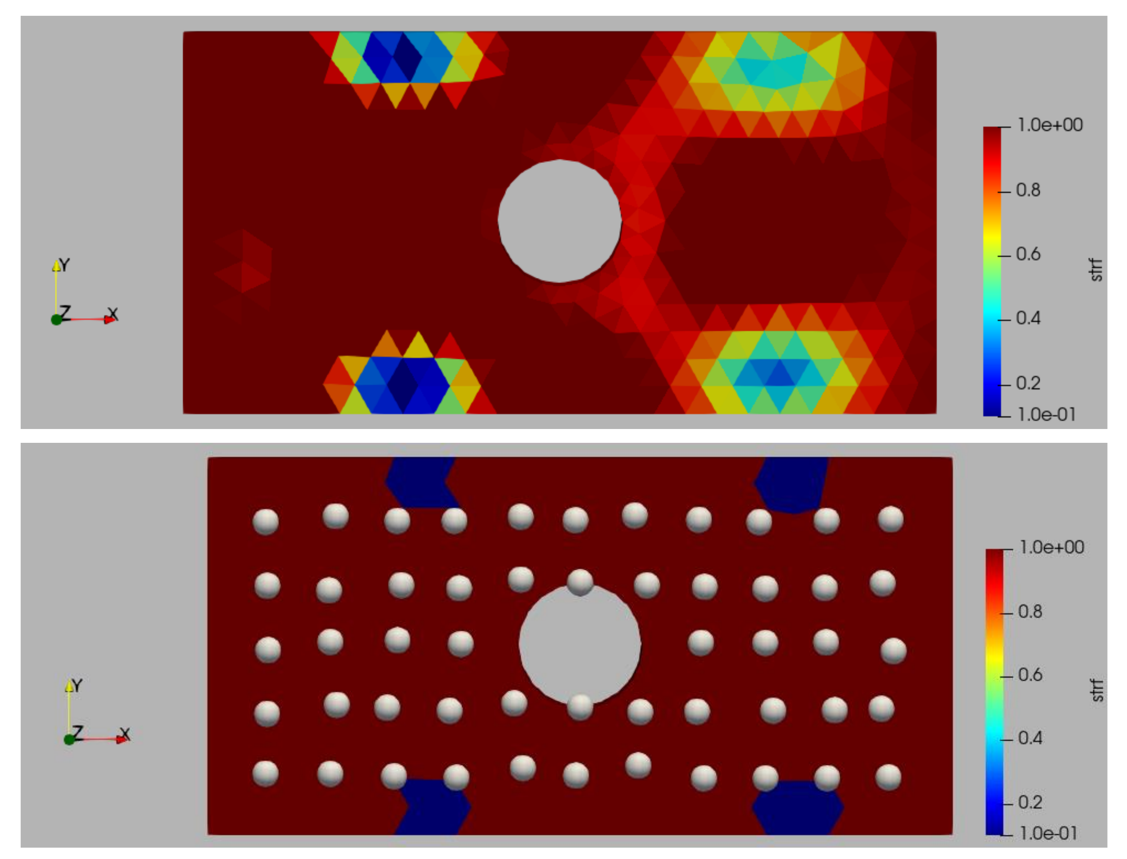
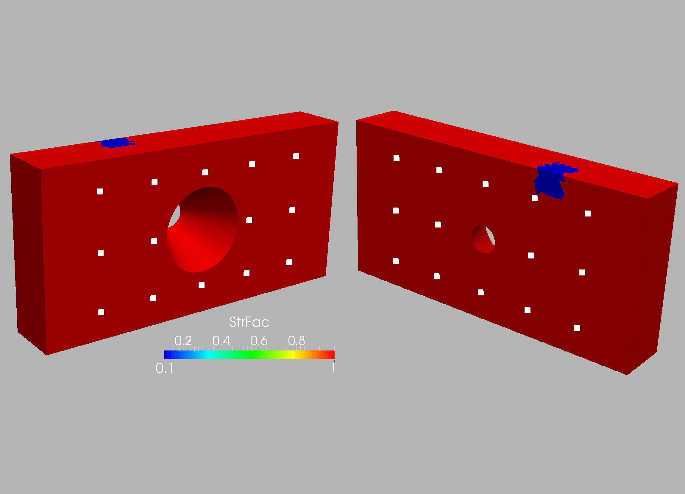
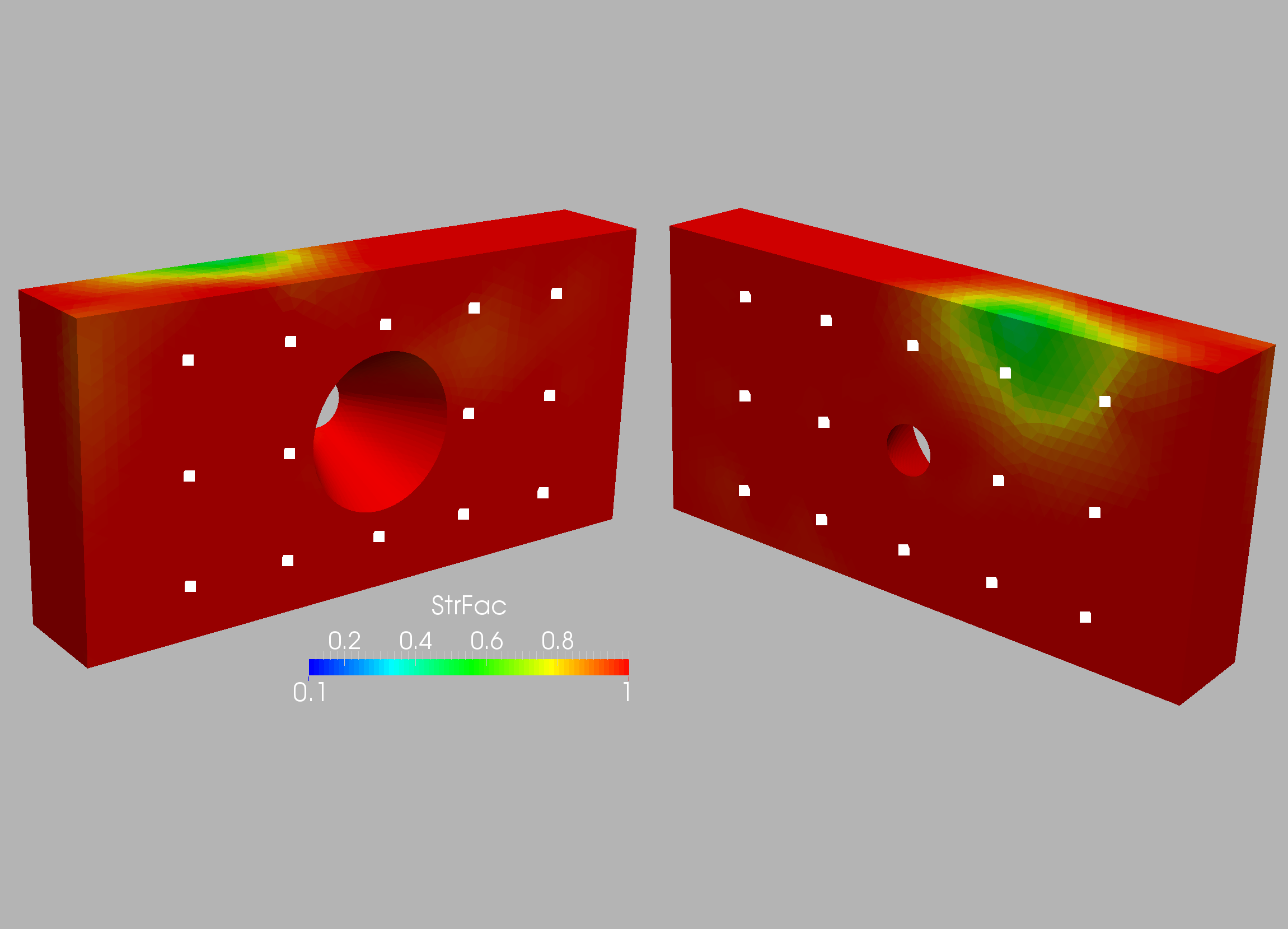
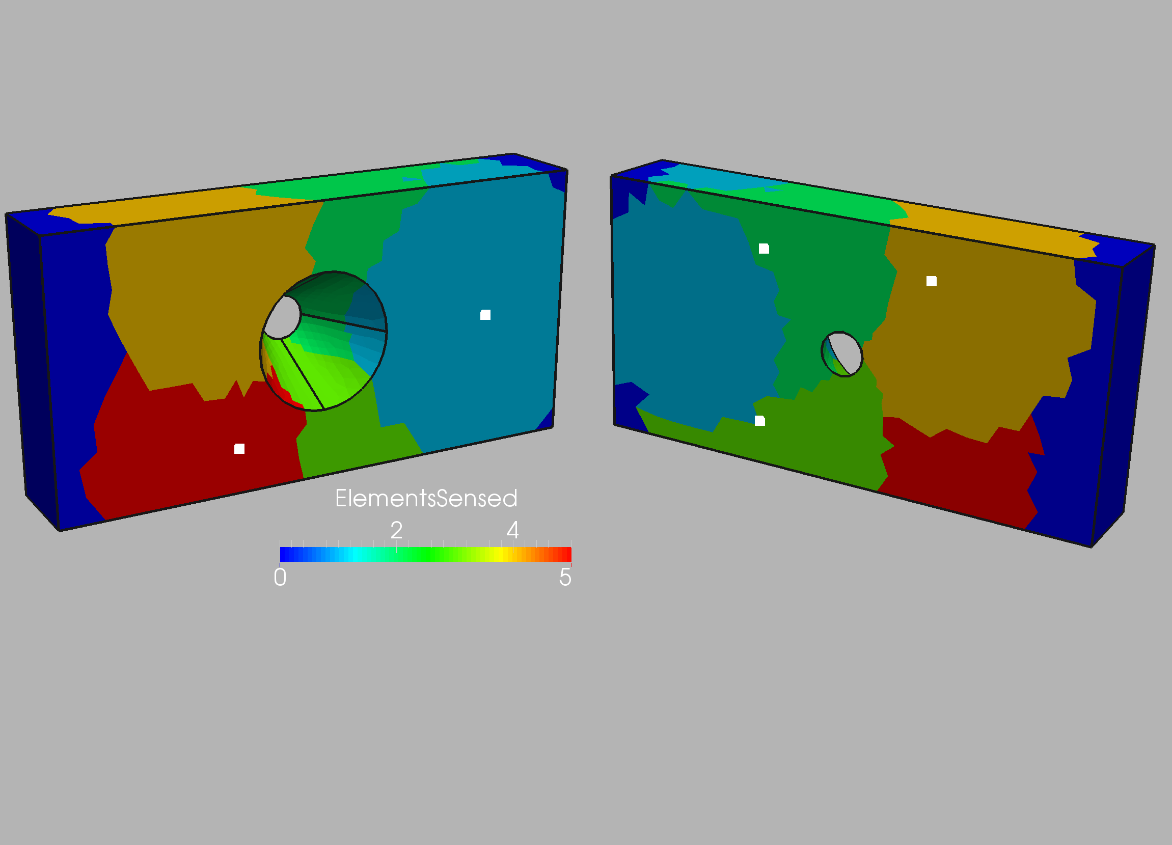
Having proven that the technique works, the optimal number of
sensors and loads were obtained. Figure 10.9 records the number
of (displacement) sensors that were able to measure/‘sense’ the
weakening of each element using the ‘forward-based’ approach.
As expected, the number is higher for
the elements close to the clamped boundary. The technique outlined
above (Section 9.3) sorted the sensors. This resulted in just 5 sensors,
whose location and ‘zone of influence’ is shown in Figures 10.10 and 10.11.
The weakening regions computed with these sensors for the two grids
are shown in Figures 10.12 and 10.13. One can see that even with this small number
of sensors the regions are well defined. The convergence history of the
cost function for these cases is plotted in Figure 10.14.
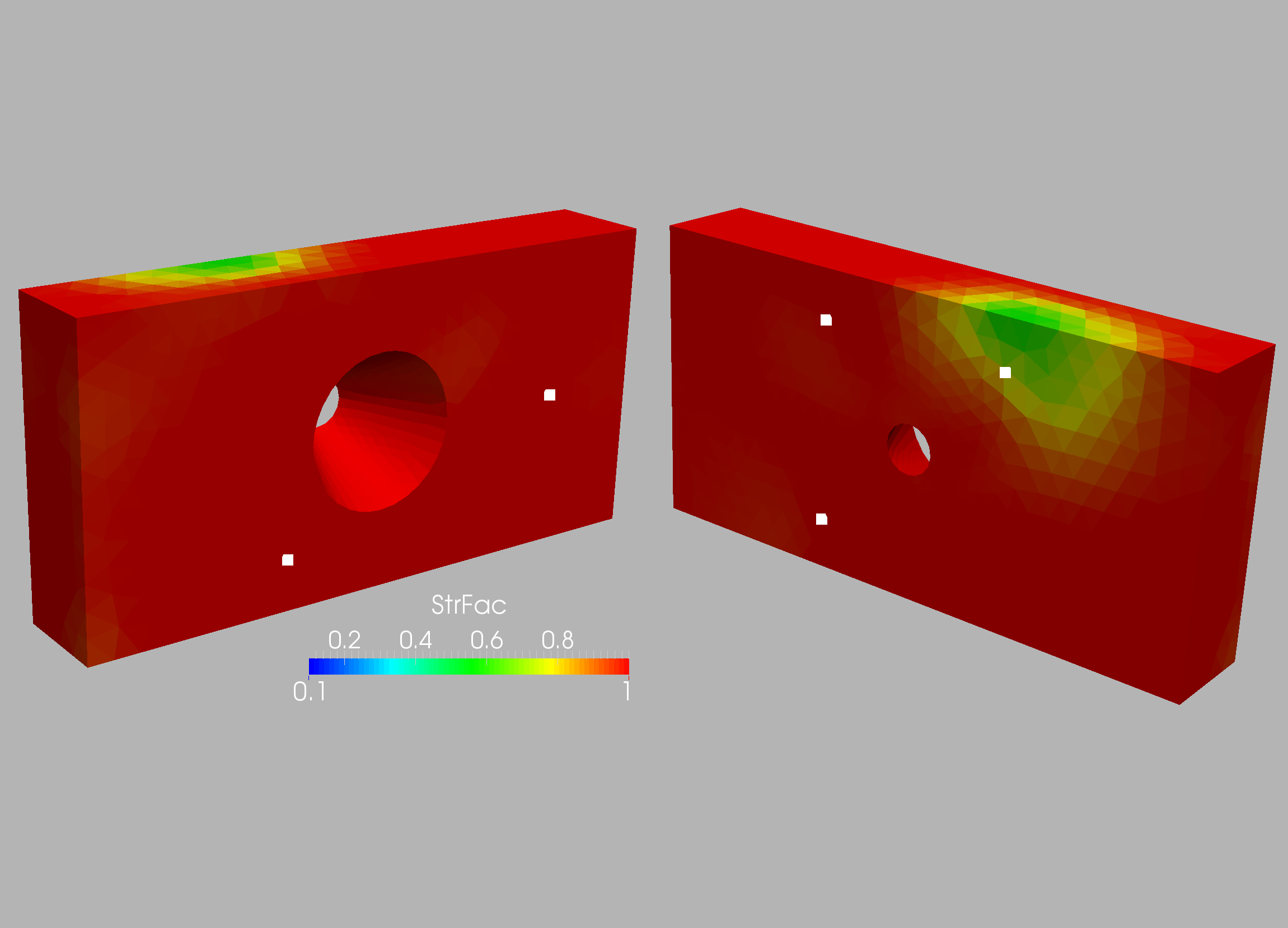
Finally, Figure 10.15 shows the number of elements with strains above
a threshold for the 2 load cases: and .
One can see that with these 2 loads cases almost all elements are
affected, so any further load cases would not lead to more information.
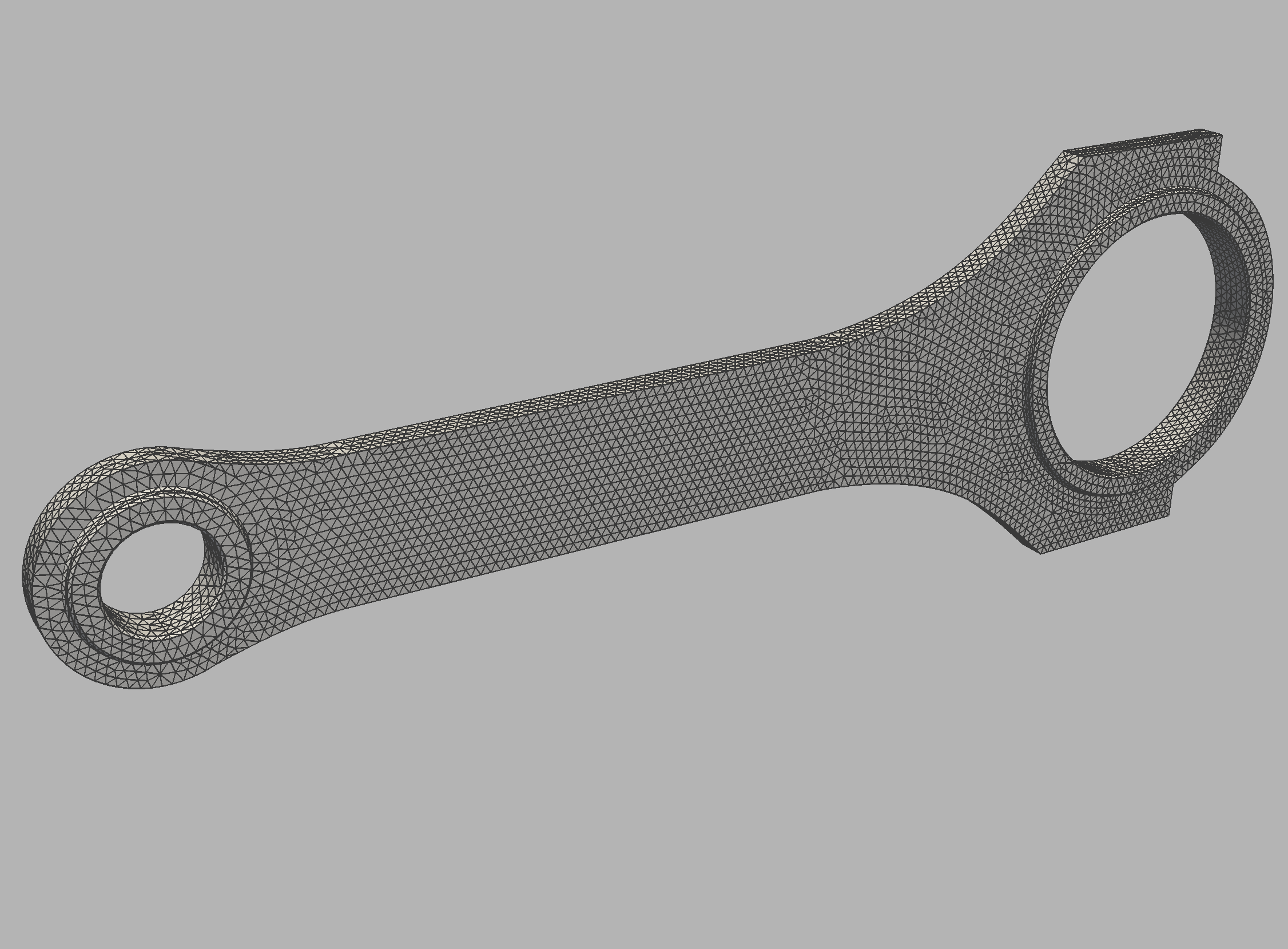
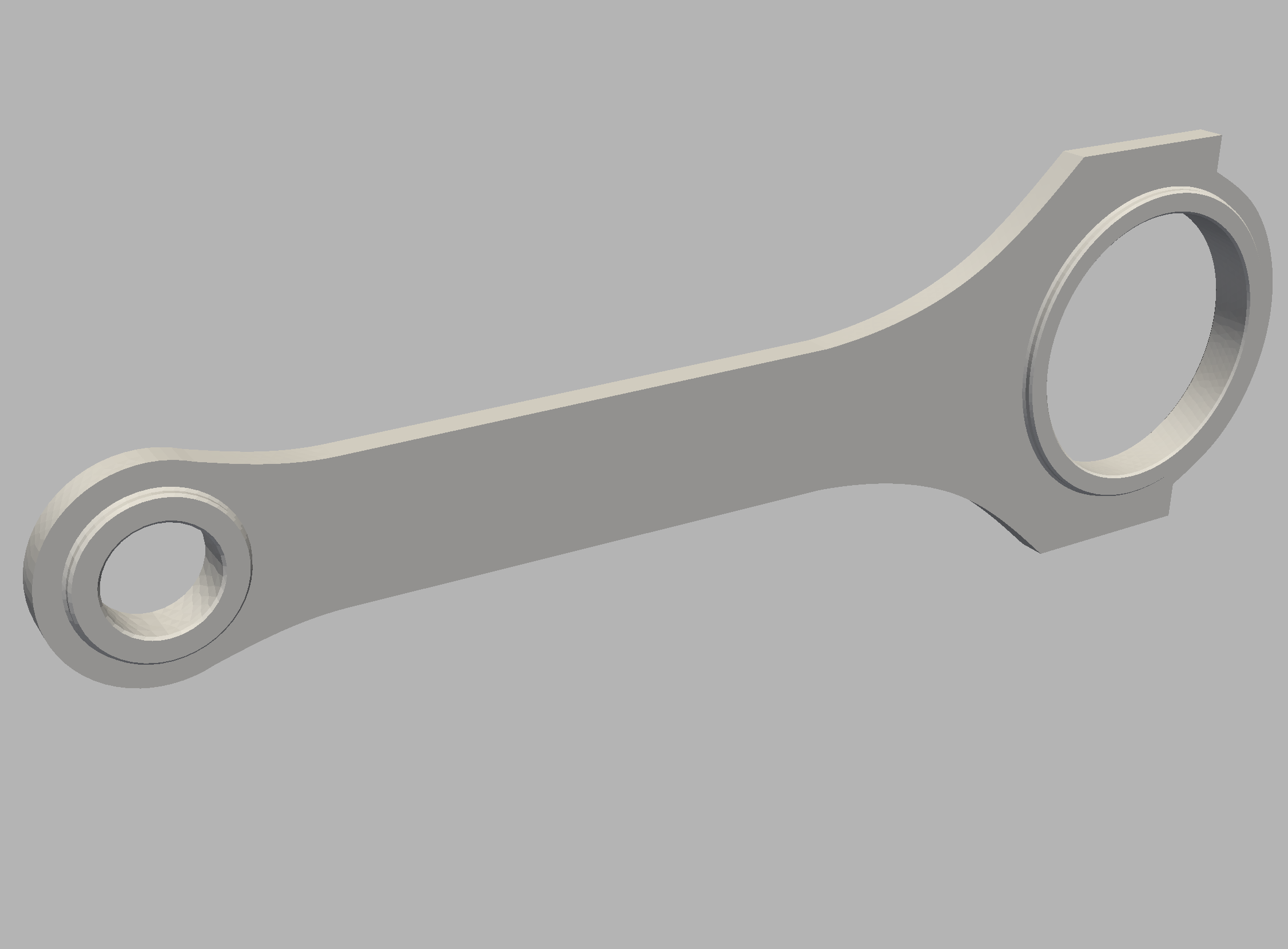
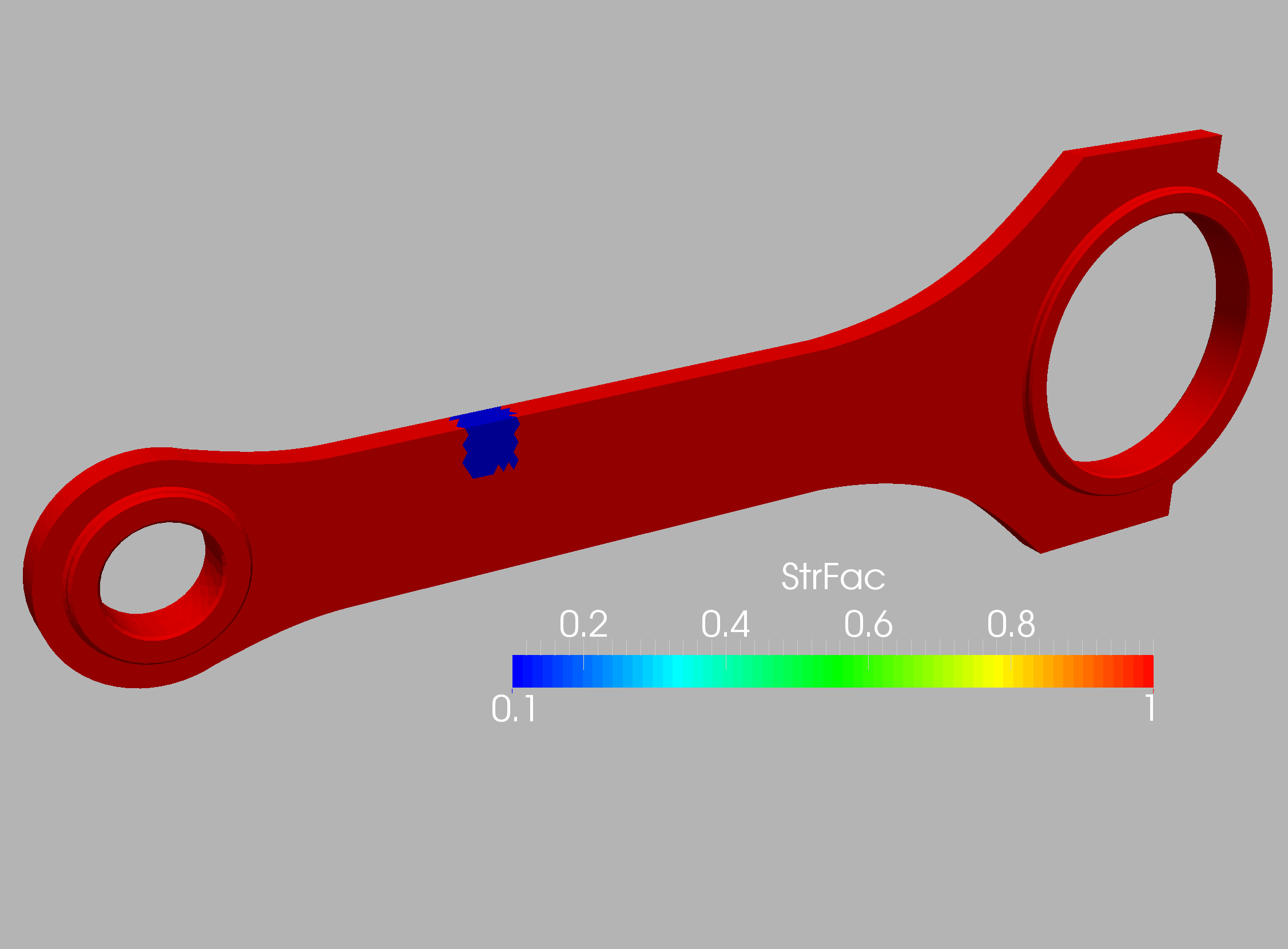
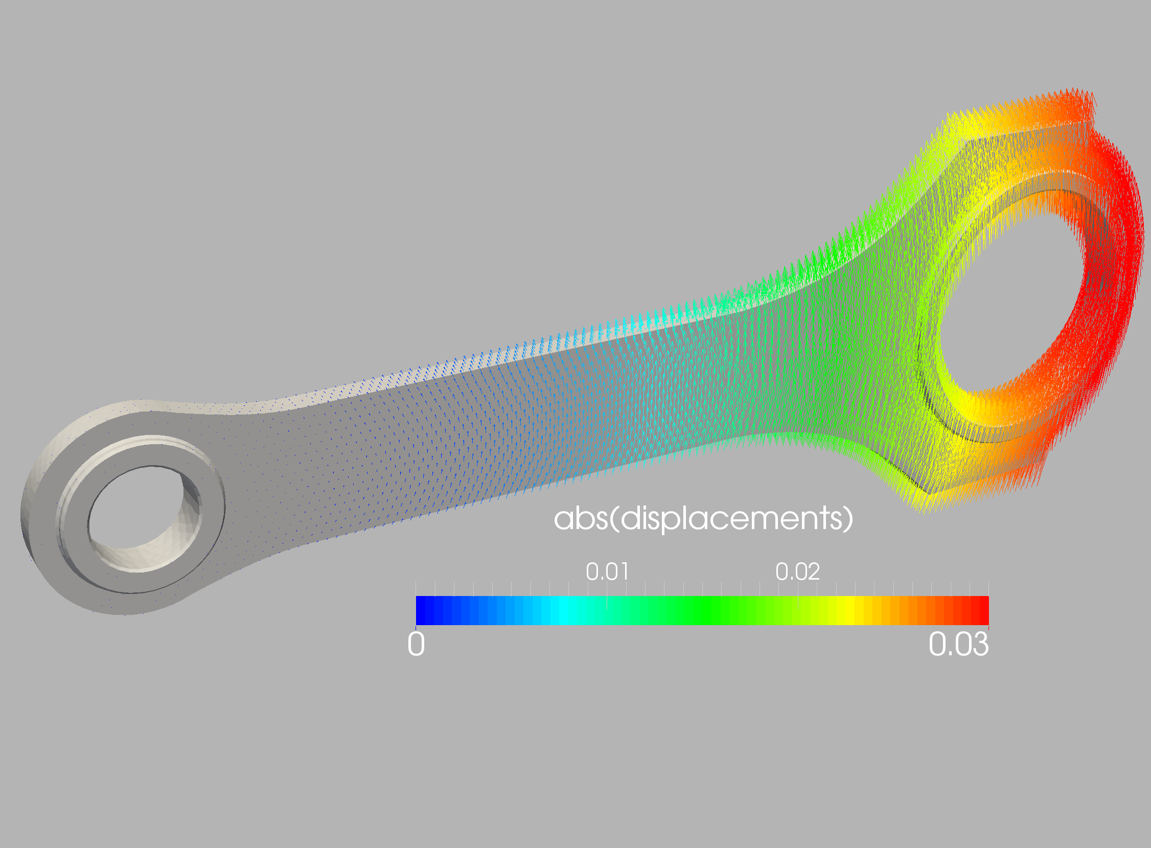
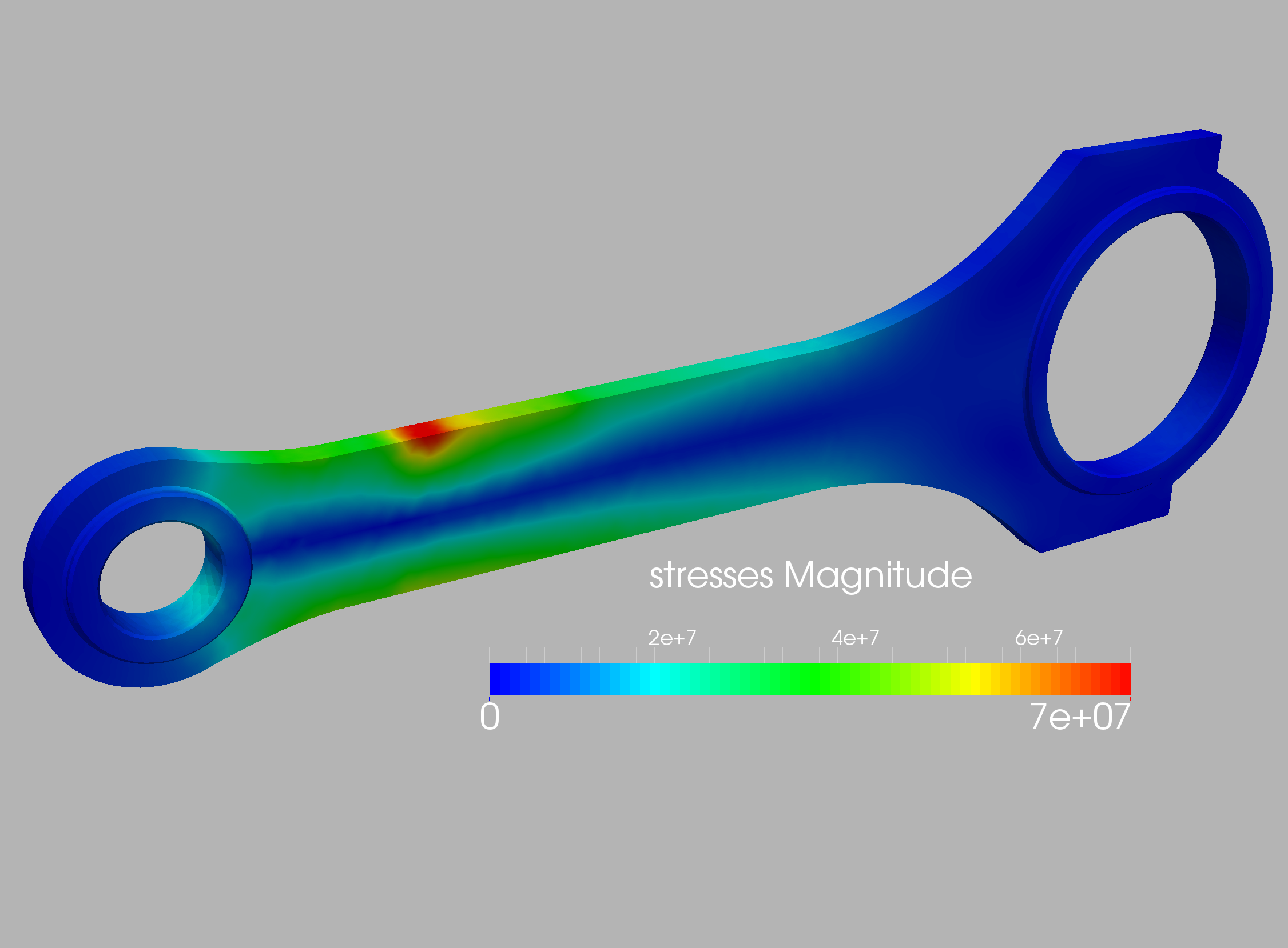
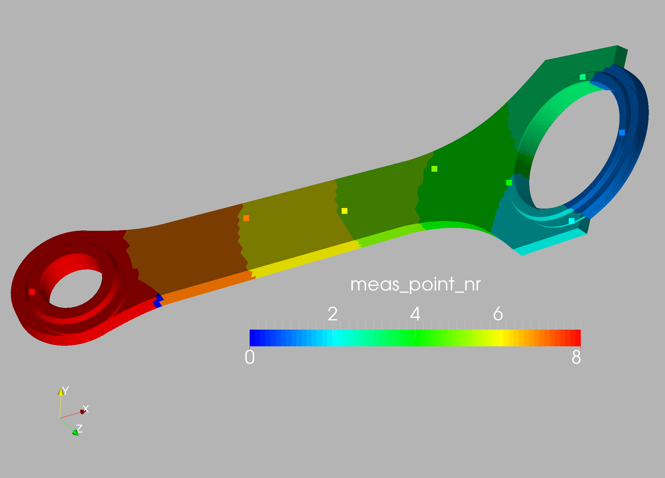
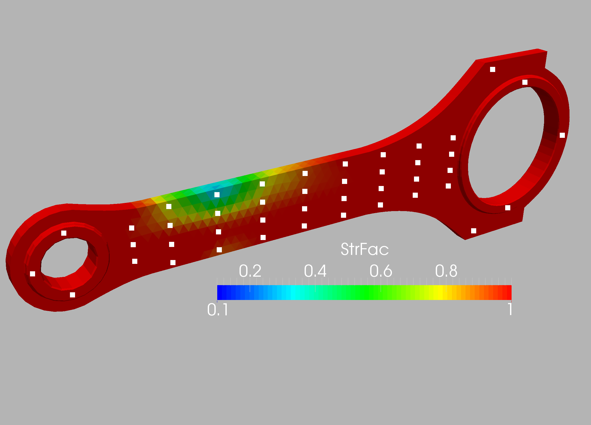
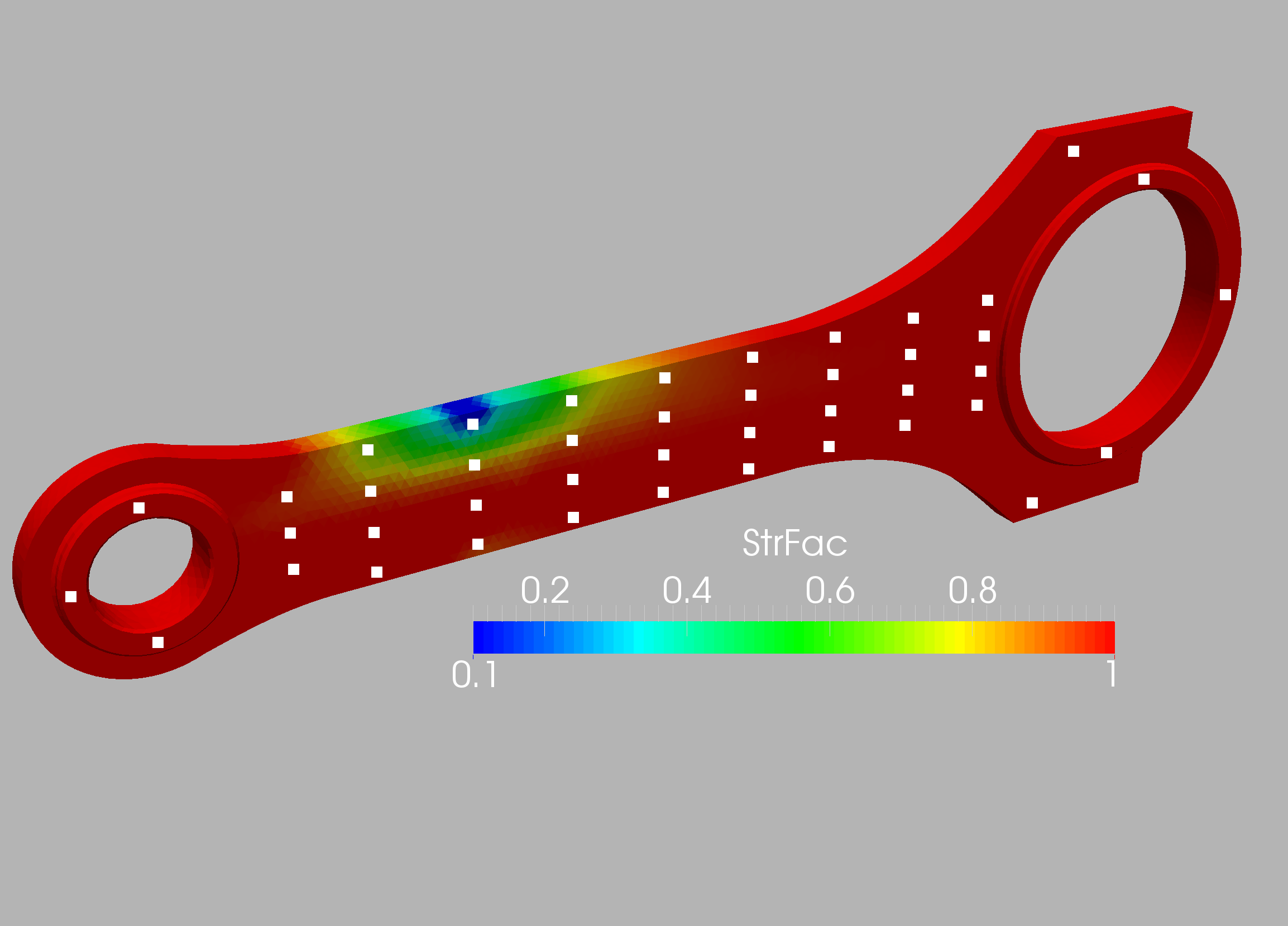
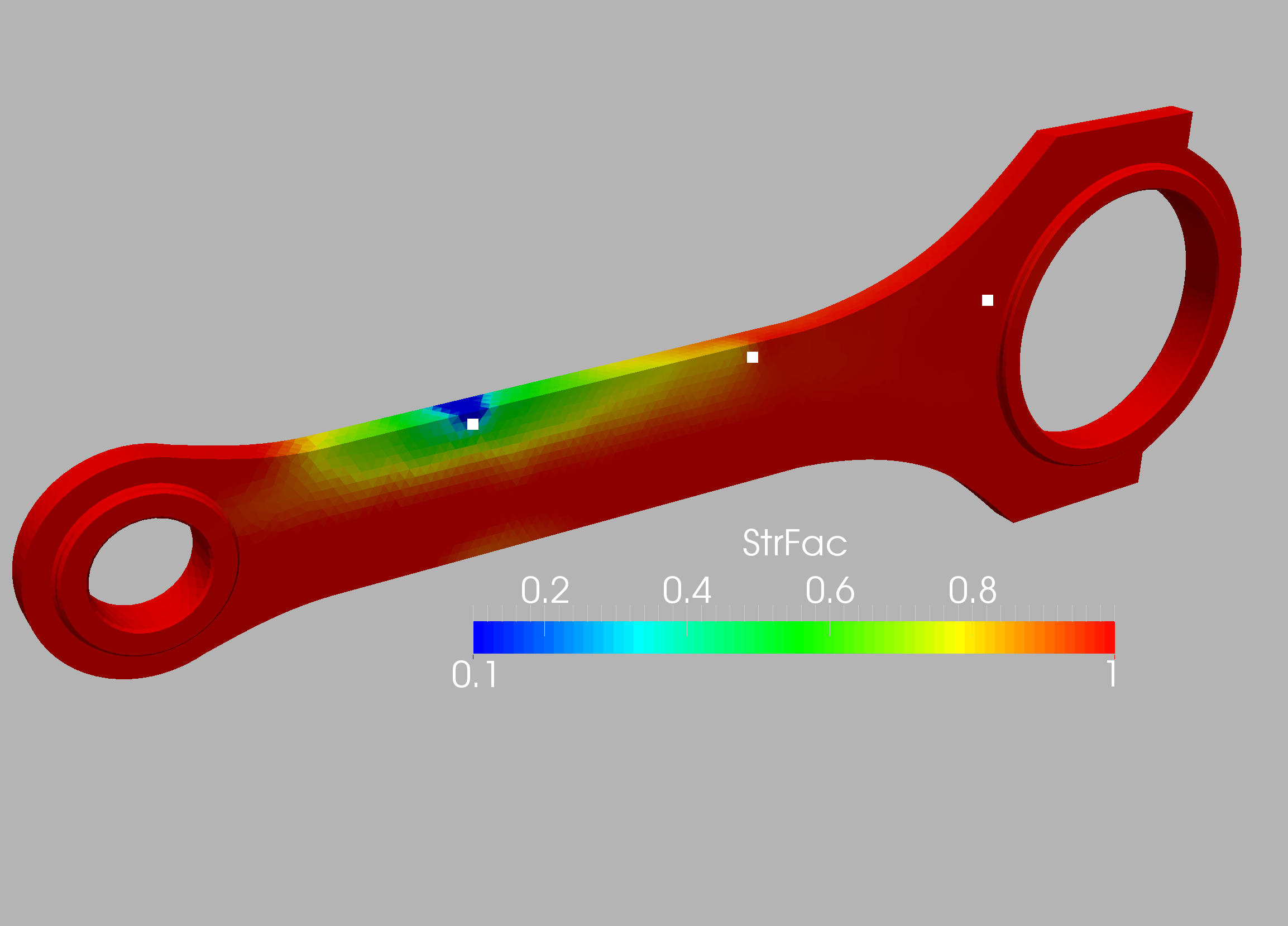
10.3. Connecting rod
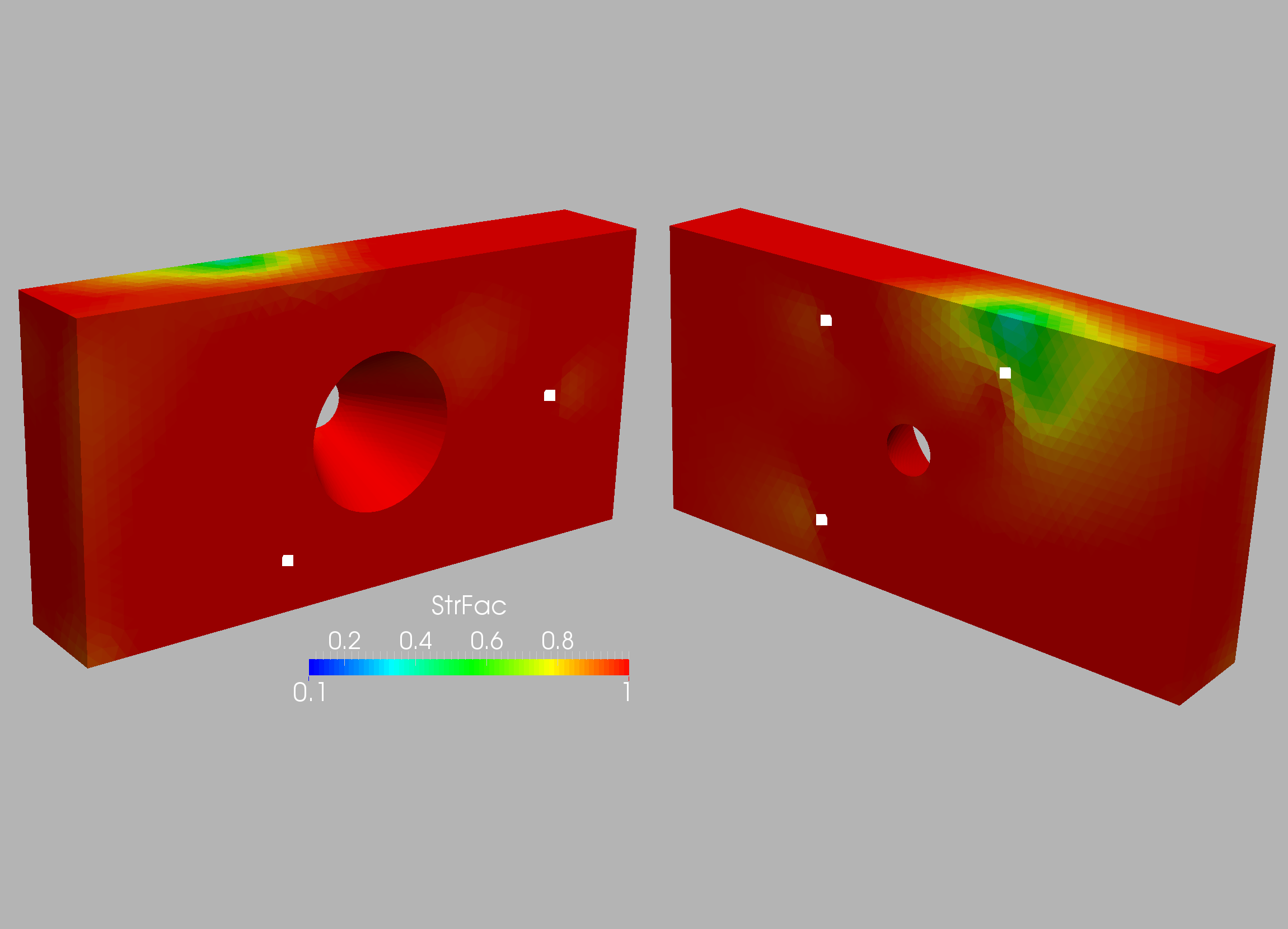
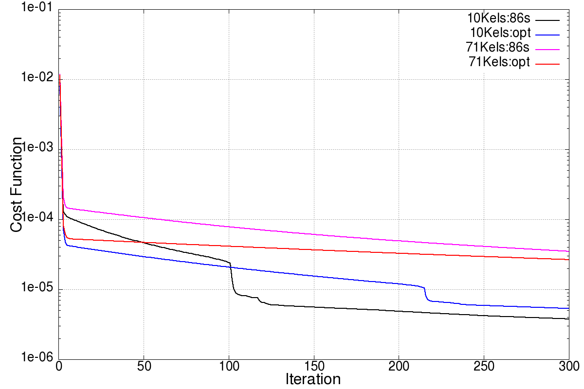
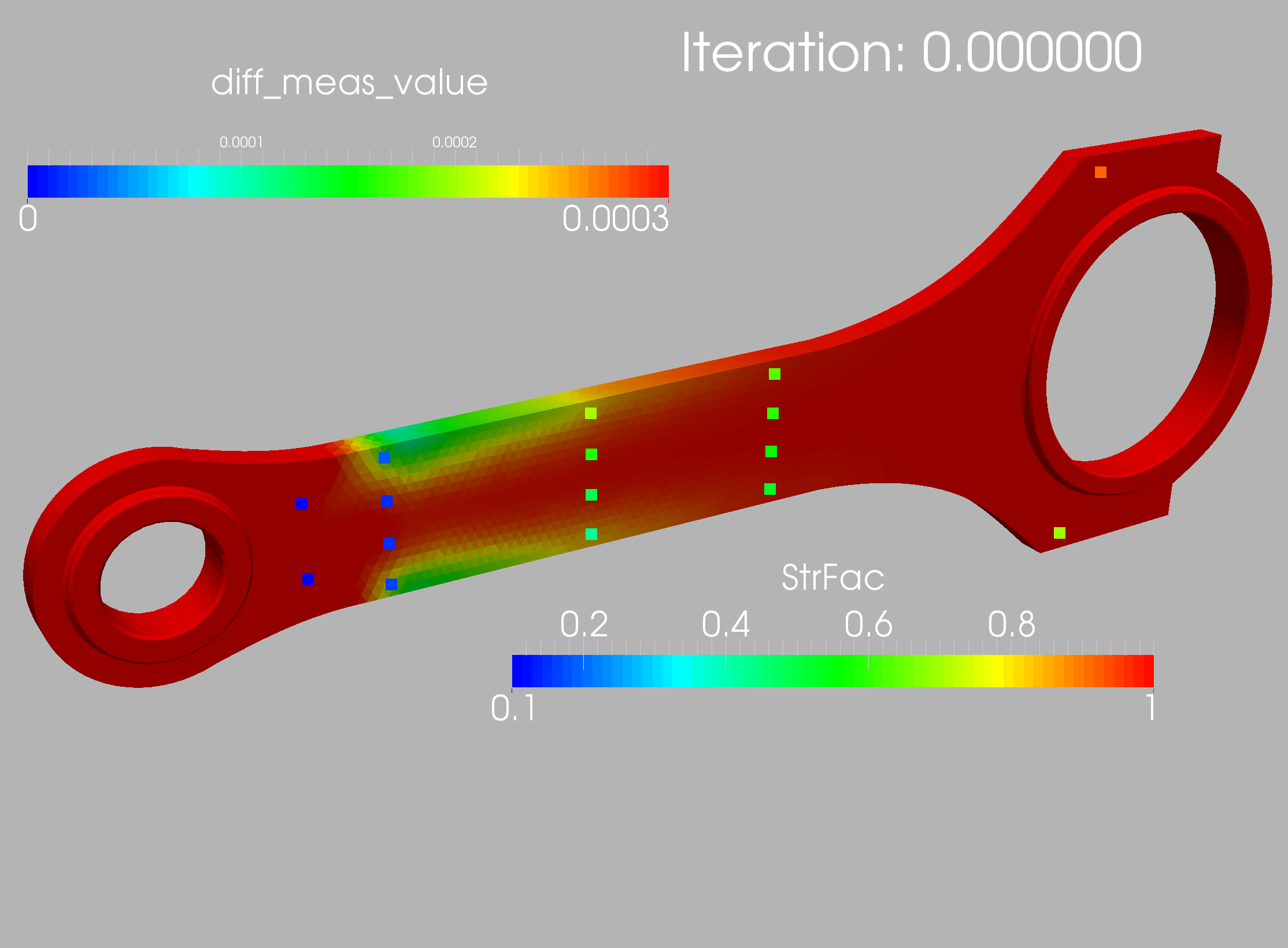
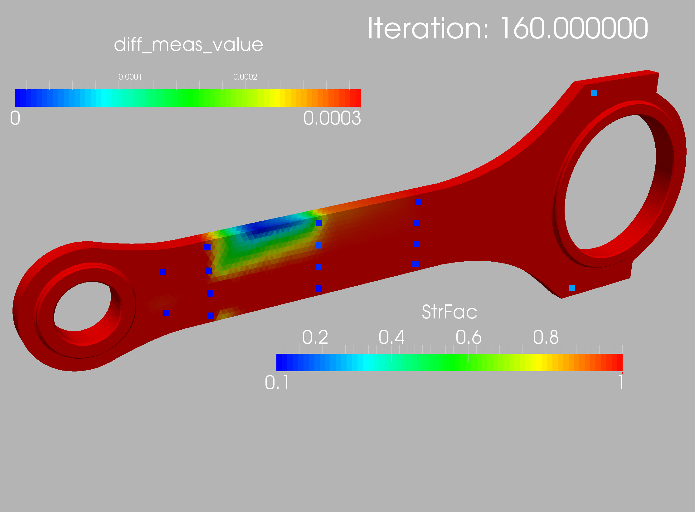
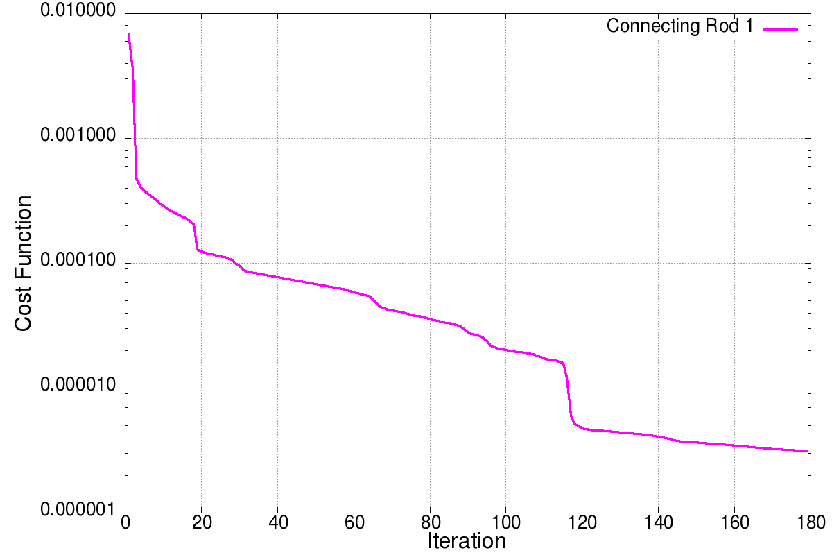
The case is shown in Figure 10.16 and considers a connecting rod typical of mechanical and aerospace engineering (e.g. to actuate flaps in wings). The two inner diameters are , and the distance between the centers is (all units in cgs). Density, Young’s modulus and Poisson rate were set to respectively. The inner part of the smaller cylinder is held fixed, while forces in the direction are applied at the larger cylinder. In order to assess the effect of mesh refinement, two different grids were employed: coarse (9.9Ktet) and medium (71Ktet). In all cases linear, tetrahedral elements were used. The surface mesh of the medium mesh is shown in Figure 10.17. In a first series of runs, 32 measuring points were placed on the connector rod surface and the target strength factor shown in Figures 10.18 was specified. Figures 10.19 and 10.20 depict the difference between the measured and computed displacements and the strength factor at iterations 0 (beginning) and 160 (end). Note the decrease in the difference between the measured and computed displacements, and the emergence of the weakened region. This is also reflected in the convergence history of the cost function (Figure 10.21). The displacements and stresses are shown in Figures 10.22 and 10.23.
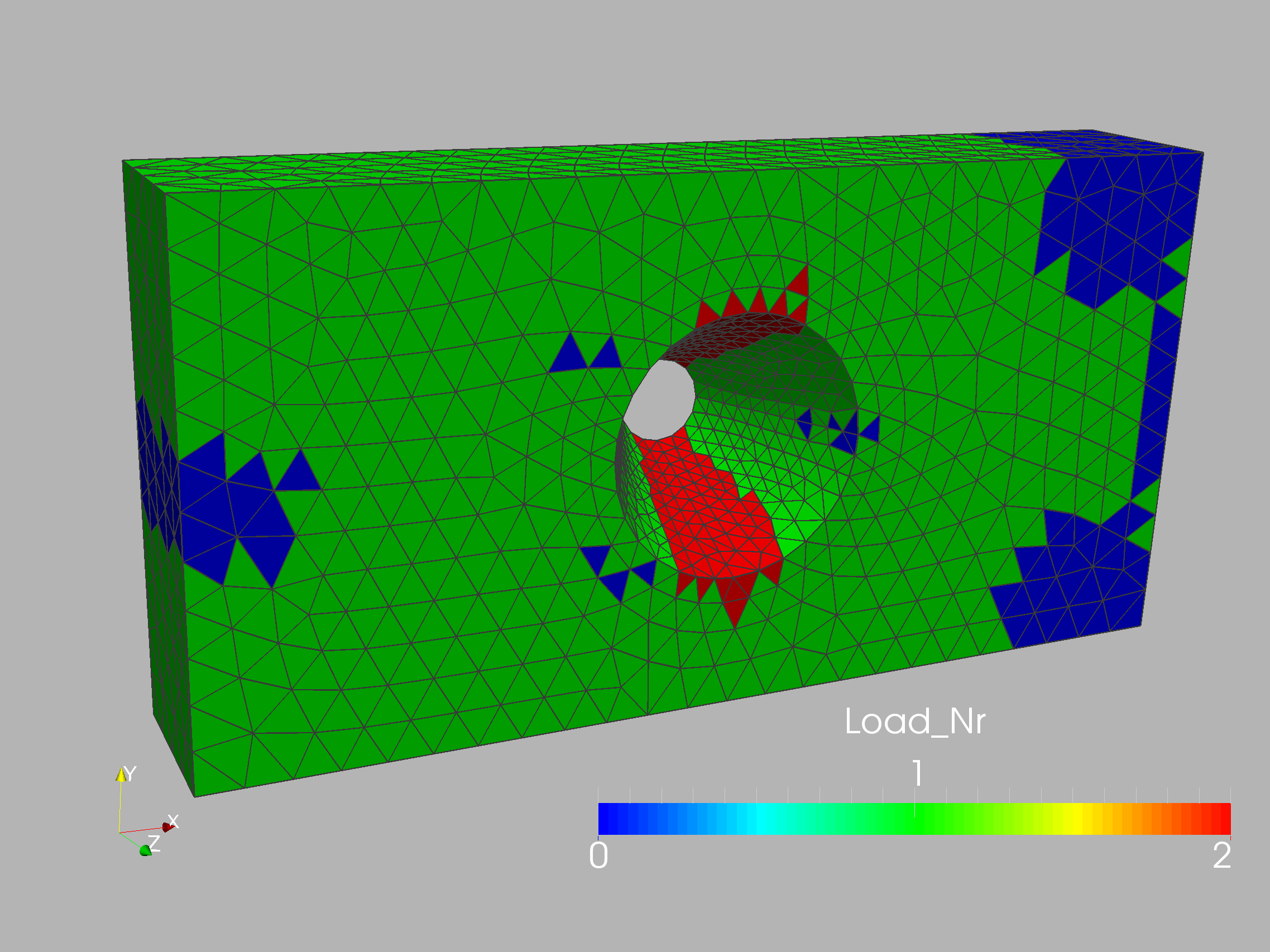
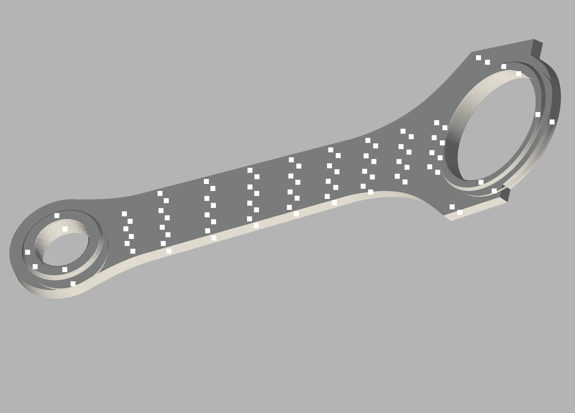
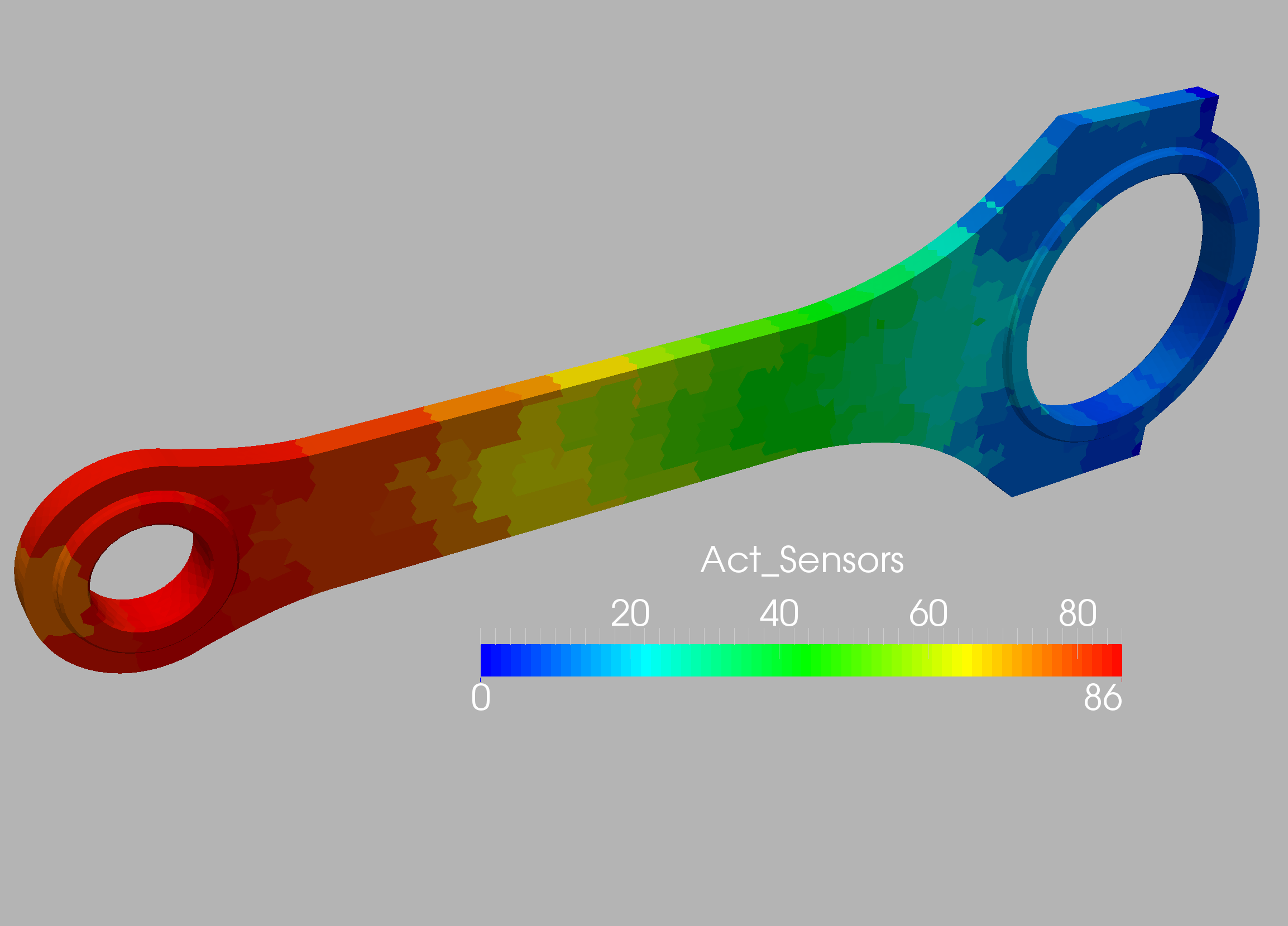
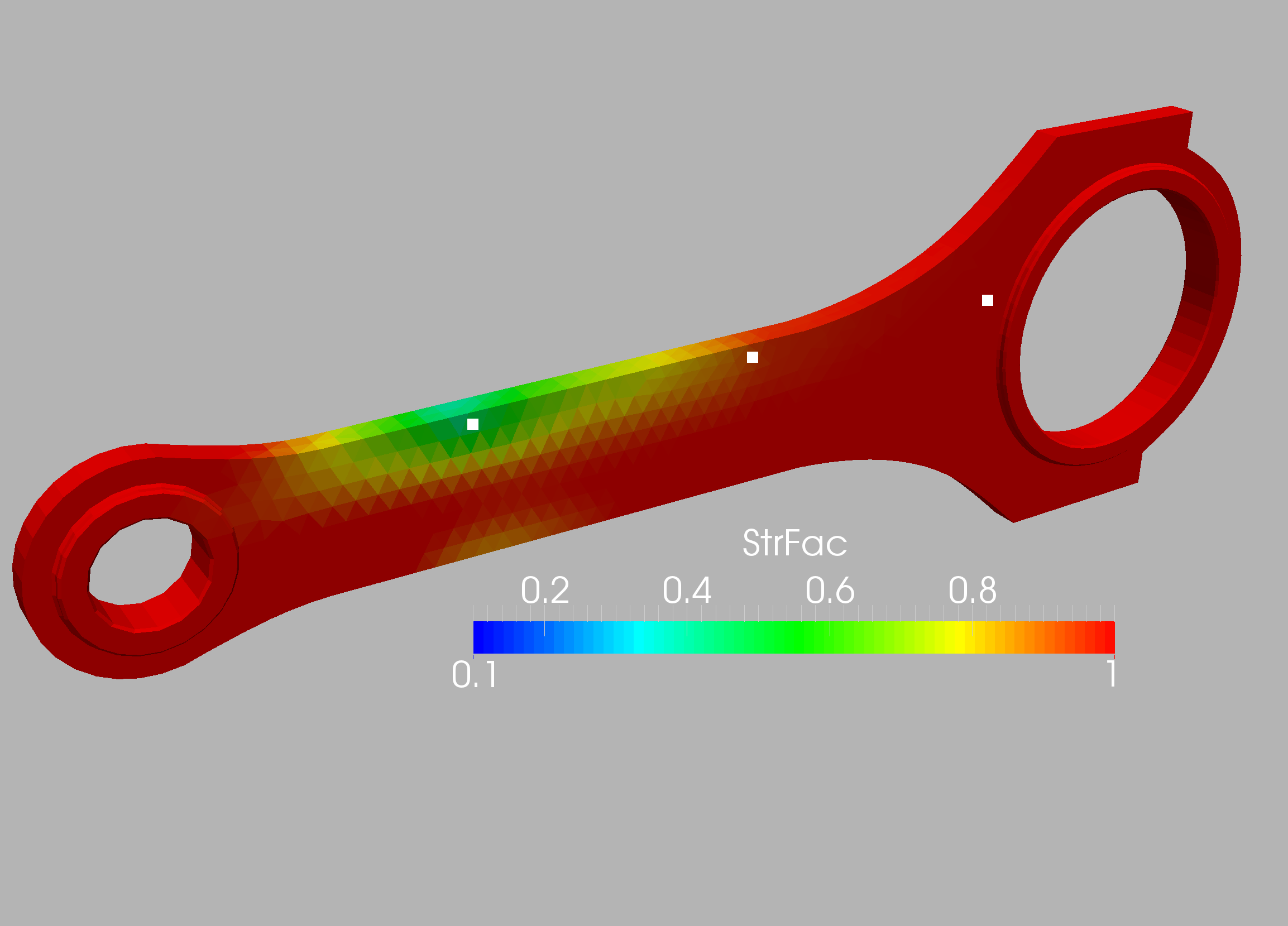
This case was analyzed further by specifying 86 measuring points (Figure 10.24) and then obtaining from these the optimal sensors using the procedures outlined above. Given that the number of elements and possible sensors was considerable, groups of elements of desired ‘group size’ of 1x1x1 cm were formed. These can be discerned in Figure 10.25, which shows the number of sensors that would ‘see’ (i.e. be activated) when a group of elements is weakened. The location of the optimal sensors obtained, as well as the region of elements each of them covers, can be seen in Figure 10.26. In order to assess the effect of mesh resolution the the weakening regions obtained using the original 86 sensor locations and the optimal 8 sensor locations for the coarse and medium meshes are compared in Figures 10.27-10.30. As expected, mesh resolution is important, and the 8 optimally placed sensors are able to detect the weakened region with high precision. This example highlights the importance of using high-definition digital twins and not simpler reduced order models (ROMs) or machine learning models (MLs) in order to localize regions of weakended material in complex structures.
11. Conclusions and outlook
An adjoint-based procedure to determine weaknesses, or, more generally
the material properties of structures has been presented. Given a
series of force and displacement/strain measurements, the material
properties are obtained by minimizing the weighted differences
between the measured and computed values. In a subsequent step
techniques to optimize the number of loadings and sensors have been
proposed and tested.
Several examples show the viability, accuracy and efficiency of
the proposed methodology.
We consider this a first step that demonstrates the viability of the
adjoint-based methodology for system identification and its use for
high fidelity digital twins [19, 9].
Many questions remain open, of which we
just mention some obvious ones:
-
-
Will these techniques work for nonlinear problems ?
-
-
Which sensor resolution is required to obtain reliable results ?
-
-
Will these techniques work under uncertain measurements ? [3]
-
-
Can one detect faulty sensors in a systematic way ?
12. Acknowledgements
This work has been partially supported by NSF grant DMS-2110263 and the Air Force Office of Scientific Research (AFOSR) under Award NO: FA9550-22-1-0248.
References
- [1] Facundo N Airaudo, Rainald Löhner, Roland Wüchner, and Harbir Antil. Adjoint-based determination of weaknesses in structures. Computer Methods in Applied Mechanics and Engineering, 417:116471, 2023.
- [2] Nizar Faisal Alkayem, Maosen Cao, Yufeng Zhang, Mahmoud Bayat, and Zhongqing Su. Structural damage detection using finite element model updating with evolutionary algorithms: a survey. Neural Computing and Applications, 30:389–411, 2018.
- [3] Harbir Antil, Drew P Kouri, Martin-D Lacasse, and Denis Ridzal. Frontiers in PDE-constrained Optimization, volume 163. Springer, 2018.
- [4] Thomas Borrvall and Joakim Petersson. Topology optimization of fluids in stokes flow. International journal for numerical methods in fluids, 41(1):77–107, 2003.
- [5] Gregory Bunting, Scott T Miller, Timothy F Walsh, Clark R Dohrmann, and Wilkins Aquino. Novel strategies for modal-based structural material identification. Mechanical Systems and Signal Processing, 149:107295, 2021.
- [6] Gregory Bunting, Scott T Miller, Timothy F Walsh, Clark R Dohrmann, and Wilkins Aquino. Novel strategies for modal-based structural material identification. Mechanical Systems and Signal Processing, 149:107295, 2021.
- [7] Peter Cawley and Robert Darius Adams. The location of defects in structures from measurements of natural frequencies. The Journal of Strain Analysis for Engineering Design, 14(2):49–57, 1979.
- [8] Ludovic Chamoin, Pierre Ladevèze, and Julien Waeytens. Goal-oriented updating of mechanical models using the adjoint framework. Computational mechanics, 54(6):1415–1430, 2014.
- [9] Francisco Chinesta, Elias Cueto, Emmanuelle Abisset-Chavanne, Jean Louis Duval, and Fouad El Khaldi. Virtual, digital and hybrid twins: a new paradigm in data-based engineering and engineered data. Archives of computational methods in engineering, 27:105–134, 2020.
- [10] Guido Dhondt. Calculix user’s manual version 2.20. Munich, Germany, 2022.
- [11] Daniele Di Lorenzo, Victor Champaney, Claudia Germoso, Elias Cueto, and Francisco Chinesta. Data completion, model correction and enrichment based on sparse identification and data assimilation. Applied Sciences, 12(15):7458, 2022.
- [12] Hansang Kim and Hani Melhem. Damage detection of structures by wavelet analysis. Engineering structures, 26(3):347–362, 2004.
- [13] Pierre Ladevèze, Djamel Nedjar, and Marie Reynier. Updating of finite element models using vibration tests. AIAA journal, 32(7):1485–1491, 1994.
- [14] Boyan Stefanov Lazarov and Ole Sigmund. Filters in topology optimization based on helmholtz-type differential equations. International Journal for Numerical Methods in Engineering, 86(6):765–781, 2011.
- [15] Rainald Löhner. Applied computational fluid dynamics techniques: an introduction based on finite element methods. John Wiley & Sons, 2008.
- [16] Rainald Löhner. Feelast user’s manual. Fairfax, Virginia, 2023.
- [17] Rainald Löhner and Harbir Antil. Determination of volumetric material data from boundary measurements: Revisiting calderon’s problem. International Journal of Numerical Methods for Heat & Fluid Flow, 2020.
- [18] NMM Maia, JMM Silva, and RPC Sampaio. Localization of damage using curvature of the frequency-response-functions. In Proceedings of the 15th international modal analysis conference, volume 3089, page 942, 1997.
- [19] Laura Mainini and Karen Willcox. Surrogate modeling approach to support real-time structural assessment and decision making. AIAA Journal, 53(6):1612–1626, 2015.
- [20] Akbar Mirzaee, Reza Abbasnia, and Mohsenali Shayanfar. A comparative study on sensitivity-based damage detection methods in bridges. Shock and Vibration, 2015, 2015.
- [21] SC Mohan, Dipak Kumar Maiti, and Damodar Maity. Structural damage assessment using frf employing particle swarm optimization. Applied Mathematics and Computation, 219(20):10387–10400, 2013.
- [22] Guillaume Puel and Denis Aubry. Using mesh adaption for the identification of a spatial field of material properties. International journal for numerical methods in engineering, 88(3):205–227, 2011.
- [23] Magdalena Rucka and Krzysztof Wilde. Application of continuous wavelet transform in vibration based damage detection method for beams and plates. Journal of sound and vibration, 297(3-5):536–550, 2006.
- [24] Maher Salloum and David B Robinson. Optimization of flow in additively manufactured porous columns with graded permeability. AIChE Journal, 68(9):e17756, 2022.
- [25] D Thomas Seidl, Assad A Oberai, and Paul E Barbone. The coupled adjoint-state equation in forward and inverse linear elasticity: Incompressible plane stress. Computer Methods in Applied Mechanics and Engineering, 357:112588, 2019.
- [26] Juan C Simo and Thomas JR Hughes. Computational inelasticity, volume 7. Springer Science & Business Media, 2006.
- [27] Fredi Tröltzsch. Optimal control of partial differential equations: theory, methods, and applications, volume 112. American Mathematical Soc., 2010.
- [28] Olek C Zienkiewicz, Robert Leroy Taylor, and Jian Z Zhu. The finite element method: its basis and fundamentals. Elsevier, 2005.