High-dimensional sliced inverse regression with endogeneity
Abstract
Sliced inverse regression (SIR) is a popular sufficient dimension reduction method that identifies a few linear transformations of the covariates without losing regression information with the response. In high-dimensional settings, SIR can be combined with sparsity penalties to achieve sufficient dimension reduction and variable selection simultaneously. Nevertheless, both classical and sparse estimators assume the covariates are exogenous. However, endogeneity can arise in a variety of situations, such as when variables are omitted or are measured with error.
In this article, we show such endogeneity invalidates SIR estimators, leading to inconsistent estimation of the true central subspace.
To address this challenge, we propose a two-stage Lasso SIR estimator, which first constructs a sparse high-dimensional instrumental variables model to obtain fitted values of the covariates spanned by the instruments, and then applies SIR augmented with a Lasso penalty on these fitted values. We establish theoretical bounds for the estimation and selection consistency of the true central subspace for the proposed estimators, allowing the number of covariates and instruments to grow exponentially with the sample size. Simulation studies and applications to two real-world datasets in nutrition and genetics illustrate the superior empirical performance of the two-stage Lasso SIR estimator compared with existing methods that disregard endogeneity and/or nonlinearity in the outcome model.
Keywords: Dimension reduction, high-dimension, instrumental variable, Lasso, measurement error, statistical genomics
1 Introduction
Sufficient dimension reduction (SDR, Ma and Zhu,, 2013; Li,, 2018) refers to a class of methods that assume the outcome depends on a set of covariates through a small number of linear combinations , with . These linear combinations are known as sufficient predictors and retain the full regression information between the response and covariates. Since the pioneering work ofLi, (1991), a vast literature has grown on different SDR approaches, ranging from inverse-moment-based and regression-based methods (e.g., Cook and Forzani,, 2008; Bura et al.,, 2022), forward regression (e.g., Xia et al.,, 2002; Dai et al.,, 2024), and semiparametric techniques (e.g., Zhou and Zhu,, 2016; Sheng and Yin,, 2016). Among the various SDR methods, sliced inverse regression (SIR, Li,, 1991) remains the most widely used due to its simplicity and computational efficiency, and as such continues to be the subject of much research (see Tan et al.,, 2018; Xu et al.,, 2022, among many others). When the number of covariates is large, it is often (further) assumed each linear combination depends only on a few covariates, i.e., the vectors are sparse. Recent literature has thus sought to combine SIR and other SDR methods with variable selection to achieve sparse sufficient dimension reduction (e.g., Lin et al.,, 2018, 2019; Nghiem et al., 2023c, ).
Much of the literature dedicated to SIR and many other SDR methods, including those mentioned above, has focused on the setting where all covariates are exogenous, and little has been done to tackle sufficient dimension reduction with endogeneity. While there is some related literature on single index models with endogenity (Hu et al.,, 2015; Gao et al.,, 2020), their approach requires approximation of the link function and is not easy to generalize to multiple index models. More specifically, letting denote a matrix, we can formulate SDR as a multiple index model
| (1) |
where denotes an unknown link function, and is random noise. In (1), the target of estimation is the column space of , also known as the central subspace. Almost all current SDR methods assume the random noise is independent of , implying where ‘’ denotes statistical independence. However, this assumption may not be reasonable in many settings where the random noise is dependent upon i.e., the covariates are endogenous.
We discuss two examples, corresponding to two data applications in Section 6, where such endogeneity can arise.
-
•
Omitted-variable bias occurs when one or more (truly important) covariate is not included in the model. A classic example relates to studying the effect of education on future earnings. Here, it is well-known future earnings depend on many other variables that are also highly correlated with education level, such as family background or an individual’s overall abilities (Card,, 1999). Such variables are usually not fully known or not collected, so the ordinary least squares fit of a regression model of earnings on education levels and other observed factors produces a biased estimate for the true effect of education (Card,, 1999). Similarly, in Section 6.1, we consider a genomic study that relates a biological outcome (e.g., body weight) to gene expressions of mice. Outside of gene expressions, there can be potentially unmeasured confounding factors, such as those related to environmental conditions, which influence both gene expression levels and the outcome.
-
•
Covariate measurement error arises when some or all covariates are not accurately measured. In the second data application in Section 6.2, we consider a nutritional study relating an individual’s health outcomes to their long–term diet, collected through 24–hour recall interviews that are subject to measurement errors (Carroll et al.,, 2006). Let denote the long-term dietary covariates. The observed data can then be modeled by , with denoting an additive measurement error independent of . In this situation, even when in the true model (1) it holds that , a naive analysis which replaces by results in endogeneity, since we can write and is correlated with . This causes naive estimators that ignore measurement errors to be biased and inconsistent.
As an aside, note that while the omitted variables lead to endogeneity because too few covariates are included in the model, Fan and Liao, (2014) argued that endogeneity also arises when a large number of covariates are included in the model i.e., is high-dimensional in (1). Specifically, for large there is a high probability at least one covariate is correlated with the random noise. For instance, genome-wide association studies typically include thousands of gene expression covariates to model a clinical outcome, and at least one gene expression is likely to correlate with random noise reflecting experimental conditions or environmental perturbations (Lin et al.,, 2015).
In this paper, we show under fairly general conditions that endogeneity also invalidates sliced inverse regression, leading to inconsistent estimates of the true column space of . To address this issue, we propose a two-stage Lasso SIR method to estimate the central space in the presence of endogeneity when valid instrumental variables are available. In the first stage, we construct a sparse multivariate linear model regressing all the covariates against the instruments and then obtain fitted values from this model. In the second stage, we apply a sparse sliced inverse regression between the response and the fitted values from the first stage, to perform simultaneous SDR and variable selection.
Addressing endogeneity via instrumental variables has been extensively studied in the econometrics and statistics literature; see Angrist and Krueger, (2001) for a review. Classical instrumental variable estimators are mostly studied with a linear model for the outcome, i.e., , and often computing a two-stage least squares estimator or a limited information maximum likelihood estimator. Hansen et al., (2008) showed in this setting that these estimators are consistent for when the number of instruments increases slowly with the sample size. More recently however, a number of methods have combined instrumental variables with regularization techniques on the covariates and/or instrumental variables to improve their performance in high-dimensional settings e.g., the Lasso-type generalized methods of moments (Caner,, 2009; Caner et al.,, 2018), focused generalized methods of moments (Fan and Liao,, 2014), and two-stage penalized least squares Lin et al., (2015); the last of these methods inspires this article. Another line of research has focused on the use of sparsity-inducing penalties to estimate optimal instruments from a large set of a-priori valid instruments (see for instance Belloni et al.,, 2012; Chernozhukov et al.,, 2015), or to screen out invalid instruments (e.g., Windmeijer et al.,, 2019). To the best of our knowledge though, none of these methods allow for the presence of non-linear link functions in the model for the response e.g., the multiple index model (1), and more broadly have not been adapted to the SDR context.
Under a setting where both the number of covariates and the number of instrumental variables can grow exponentially with sample size , we derive theoretical bounds on the estimation and selection consistency of the two-stage Lasso SIR estimator. Simulation studies demonstrate the proposed estimator exhibits superior finite sample performance compared with a single stage Lasso SIR estimator when endogeneity is present but ignored, and the two-stage regularized estimator proposed by Lin et al., (2015) when the outcome model is non-linear in nature. We apply the proposed method to two real data applications studying the effects of different nutrients on the cholesterol level (covariate measurement error), and for identifying genes that are relevant to the body weight of mice (omitted variable bias).
The remainder of this article is structured as follows. In Section 2, we briefly review two versions of sliced inverse regression and prove that endogeneity causes SIR to be inconsistent for estimating the target subspace. In Section 3, we formulate the proposed two-stage Lasso estimators, and derive their theoretical properties in Section 4. Section 5 presents simulation studies to compare the performance of the proposed estimator with existing methods, while Section 6 discusses two data applications Finally, Section 7 offers some concluding remarks.
2 SIR and endogeneity
In this section, we first establish the setting of interest, namely a high-dimensional multiple index model for the response along with a high-dimensional linear instrumental variable model for the covariates characterizing endogeneity. We then review SIR and a version augmented with the Lasso penalty (Section 2.1), and then demonstrate inconsistency of SIR under endogeneity in Section 2.2.
Before proceeding, we set out some notation to be used throughout the paper. For any matrix with elements , let , , and denote the matrix -norm, -norm, and element-wise maximum norm, respectively. Also, let denote the -operator norm, i.e. the largest singular value of . For any vector with elements , let and and denote its Euclidean norm, norm, and norm, respectively. Finally, for an index set , let denote the subvector of formed with the elements of whose indices , denote its cardinality, and denote its complement.
Consider a set of independent observations where, without loss of generality, we assume . Each triplet follows the multiple index model (1) coupled with the linear instrumental variable model. That is, the full model is given by
| (2) |
where , , denotes the random noise for the outcome model, and denotes the random noise for the instrumental variable model. The vector is assumed to have mean zero and finite covariance matrix , whose diagonal elements are denoted by for . To characterize endogeneity between and , the off-diagonal elements in the last row and column of are generally non-zero, while the instrumental variable satisfies for all .
We seek to estimate the column space of , when the dimensions and are growing exponentially with the sample size . A common assumption in such settings is that sparsity holds. Specifically: i) each covariate depends upon only a few instrumental variables, such that in the instrumental variable model the th column of is a sparse vector with at most non-zero elements, where is bounded, and ii) the multiple index model is sparse such that depends only on covariates i.e., at most rows of are non-zero row vectors. Equivalently, if denotes the corresponding projection matrix, then only diagonal elements of are non-zero. Without loss of generality, we assume i.e., the first covariates indexes this set of non-zero elements, or, equivalently, the support set of the column space of . We let and denote the matrix of covariates, matrix of instrumental variables, and vector of responses, whose th rows are given by , and , respectively. Let and denote the th column of and , respectively. For the remainder of this article, we use , and to denote the random variables from which is drawn.
2.1 Review of sliced inverse regression and Lasso SIR
The sliced inverse regression or SIR estimator (Li,, 1991) of the column space of was developed under the assumption that the random noise is independent of the covariates . The key assumption of SIR is the following linearity condition, which is satisfied when the covariates follow an elliptical distribution.
Condition 2.1.
The conditional expectation is a linear function of .
Under this condition, the population foundation for SIR is that the inverse regression curve is contained in the linear subspace spanned by (Theorem 3.1, Li,, 1991). As a result, letting denote the set of eigenvectors associated with the largest eigenvalues of , we have for . Since , we can estimate from estimates of and . This approach to estimation for SIR is recommended by Li, (1991), and used by many authors in the literature (Tan et al.,, 2018; Zou,, 2006), although it is not the only approach possible (Lin et al.,, 2019).
In more detail, suppose we estimate by the sample covariance . When , this sample covariance matrix is not invertible, but the Lasso SIR estimator generally does not require such invertibility as we will see in a moment. Then, partitioning the data into non-overlapping slices based on the order statistics of , we compute the sample covariance matrices within each slice and average them to form
where denotes the slice size and we have assumed to simplify the notation. Zhu et al., (2006) showed that can be rewritten in the form
and denotes the vector of ones. We can then estimate by , where . It follows that the eigenvector can be estimated by , the eigenvector associated with the th largest eigenvalue of .
For settings where is large and is sparse, consider replacing the population relationship by its sample counterpart. Then we have , from which Lin et al., (2019) proposed the Lasso SIR estimator
| (3) |
with the pseudo-response vector , and denotes a tuning parameter for the th pseudo-response. The Lasso penalty can be straightforwardly replaced by a more general sparsity-inducing penalty (e.g., the adaptive Lasso penalty in Nghiem et al., 2023c, ). With an appropriate choice of , the solution is sparse, facilitating variable selection for each dimension of the estimator. Variable selection for the estimated central subspace is obtained by taking the union of the estimated support sets across all dimensions .
2.2 Inconsistency of SIR under endogeneity
When endogeneity is present, the inverse regression curve in no longer guaranteed to lie in the subspace spanned by , even when Condition 2.1 holds for the marginal . The following proposition establishes this result in the case follows a multivariate Gaussian distribution.
Proposition 1.
Assume follows a dimensional Gaussian distribution. Let . Then the inverse regression curve is contained in the linear subspace spanned by if and only if , where denotes the column space of .
In Proposition 1 the matrix is the coefficient vector of the best linear predictor of from , so this proposition implies that even when endogeneity is present, the population foundation for SIR only holds when the random noise can be predicted from the linear combination itself. This condition is obviously restrictive, since it requires the same set of linear combinations to be used to predict both the response and the random noise .
When the condition in Proposition 1 is not satisfied, the Lasso SIR estimator in (3) is generally not a consistent estimator of the column space of . The following proposition makes this precise in a simple setting where the number of covariates is fixed and the penalization is asymptotically negligible.
Proposition 2.
Let denote the Lasso SIR estimator formulated in (3) with tuning parameters for all as . Then, , where , with the eigenvectors of . As a result, if the covariance vector , then is inconsistent for the column space of , and as .
Proposition 1 implies that when the covariance vector , endogeneity invalidates SIR as an estimator of the overall central subspace. Note this does not necessarily imply selection inconsistency, i.e. inconsistency in estimating the support set corresponding to the non-zero elements of the diagonal of . Selection consistency can still be achieved if the column space of has the same support as that of ; see the Supplementary Material S1 for an empirical demonstration. On the other hand, when the number of covariates grows then it is unlikely will share the same support as . This motivates us to propose a new SIR method to handle endogeneity in high dimensional settings.
3 A two-stage Lasso SIR estimator
To overcome the general inconsistency of the SIR estimator when endogeneity is present, we propose a two-stage approach for SDR and variable selection inspired by the classical two-stage least-squares estimator (Hansen et al.,, 2008). Let , the conditional expectation of the covariates on the instruments. We first impose a new linearity condition to ensure the conditional expectation behaves similarly to when no endogeneity is present.
Condition 3.1.
The conditional expectation is a linear function of .
Despite being stronger than Condition 2.1, Condition 3.1 is satisfied when the linear instrument variable model holds and the -dimensional random vector follows an elliptical distribution. In our simulation study in Section 5, we show the proposed method still exhibits reasonable performance even when this condition is not satisfied, for example, when is binary. We then have the following result.
Lemma 1.
Assume Condition (3.1) holds. Then the quantity is contained in the linear subspace spanned by .
Note the covariance matrix need not be of full-rank and invertible: this occurs if the number of endogenous covariates is greater than the number of instruments . Nevertheless, Lemma 1 motivates us to propose a two-stage Lasso SIR (abbreviated to 2SLSIR) estimator for the column space of , assuming its entries are sparse, based on the observed vector , covariate matrix , and instrument matrix . As we shall see, while theoretically we need to understand the behavior of its inverse, computationally does not have to be inverted to construct the 2SLSIR estimator.
The two stages of the 2SLSIR estimator are detailed as follows.
-
•
Stage 1: Identify and estimate the effects of the instruments , and subsequently obtain the predicted values of the covariates . To accomplish this, we fit a multivariate instrumental variable model given by the second equation in (2), with the covariates being the -dimensional response and instruments being the -dimensional predictor. We assume each endogenous covariate depends only on a few instrumental variables (Belloni et al.,, 2012; Lin et al.,, 2015), thus motivating a sparse first-stage estimator that can be computed in parallel by computing the estimated th column as
where denotes the tuning parameter for the th covariate in the first stage. After the estimator is formed, we construct the first-stage prediction matrix .
-
•
Stage 2: Compute a sparse estimator for the column space of by applying the Lasso SIR estimator (3) with the response vector and the first-stage prediction matrix , Specifically, let , and define the pseudo-response vector , where denotes the eigenvector associated with the th largest eigenvalue of , and is defined as in Section 2.1. Then the 2SLSIR estimator for the th column of is given by
(4) where is a tuning parameter for the th pseudo-response in the second stage.
We highlight that, computationally, both stages can be implemented straightforwardly and in parallel using standard coordinate descent algorithms. In this paper, we apply the R package glmnet (Friedman et al.,, 2010) to implement the 2SLSIR estimator, and select the tuning parameters and via default standard ten-fold cross-validation as available in the software.
4 Theoretical analysis
We study the properties of the 2SLSIR estimator for the column space of under the multiple index model (2), when the dimensionality of the covariates and instruments can grow exponentially with sample size . Compared with the theoretical results for the linear outcome model in Lin et al., (2015) say, the major challenge here lies in the nonlinear nature of the conditional expectation , and subsequently the behavior of the eigenvectors corresponding to the covariance matrix which require more complex technical developments. We will use , , to denote generic positive constants. Also, without loss of generality, we assume each column of the instrumental matrix is standardized such that for .
Following the notation in Wainwright, (Chapter 7, 2019), we say an matrix satisfies a restricted eigenvalue (RE) condition over a set with parameters if for all . Also, for a vector let be the support set of . Let , where we recall are the diagonal elements of the covariance matrix corresponding to . We assume each and hence to be a constant with respect to sample size.
The following technical conditions on the distribution of the instruments and the conditional expectation are required.
Condition 4.1.
The instrument random vector is sub-Gaussian with a covariance matrix , such that for any there exists a constant such that , where and .
Condition 4.2.
There exists a constant such that .
Condition 4.3.
The quantities satisfy .
The sub-Gaussian condition is often imposed in high-dimensional data analysis (e.g. Tan et al.,, 2018; Wainwright,, 2019; Nghiem et al., 2023b, ). Note a direct consequence of Condition 4.1 is that the instrumental matrix satisfies the RE condition with parameter with high probability when for some finite (Banerjee et al.,, 2014); we will condition on this event in our development below. Furthermore, letting denote the sample covariance of data, then
| (5) |
with probability at least (see Ravikumar et al.,, 2011; Tan et al.,, 2018, for analogous results). Condition 4.2 is also imposed in the theoretical analysis of the two-stage penalized least square methods in Lin et al., (2015), and is necessary to bound the estimation error from the first stage. Finally, in the theoretical analysis below we allow the number of covariates and instruments , and the sparsity levels and to depend on the sample size , subject to the rate of growth of these parameters dictated by Condition 4.3. As a special case, if and are bounded then and can grow exponentially with .
4.1 First stage results
In the first stage of the 2SLSIR estimation procedure, each column of the matrix is a Lasso estimator from the regression of on the design matrix . We obtain the following result as a straightforward application of Banerjee et al., (2014); all proofs are provided in the Supplementary Materials S2.
Theorem 1.
Theorem 1 allows us to establish estimation consistency for the column space of in the following section.
4.2 Second stage results
In the second stage, we compute the Lasso SIR estimator using the outcome and the values obtained from the first stage. We require additional technical assumptions.
Condition 4.4.
There exists a constant such that , where is the th largest eigenvalue of .
Condition 4.5.
The covariance matrix satisfies the RE condition with parameters (, for some constant and .
Condition 4.6.
Let be the order statistics of the sample response data . Let and let denote the collection of all the -point partitions on the interval . We assume the vector-valued random variable to have a total variation of order . That is, for any fixed , we have
Condition 4.4 is analogous to the coverage condition imposed in the SIR literature for (e.g., Li,, 1991). Condition 4.5 ensures the loss function corresponding to the second stage of the proposed Lasso SIR estimator does not have too small curvature, and is similar to a condition imposed by Lin et al., (2015) for the two-stage penalized least square method. Finally, Condition 4.6 controls the smoothness of the conditional expectation . Such a similar condition is used in Tan et al., (2018) when no endogeneity is present, and similar conditions on the total variation have been introduced in much earlier work on SIR (e.g., Hsing and Carroll,, 1992; Zhu et al.,, 2006).
We first consider the case of i.e., the single index model version of (2). Here, Lemma 1 implies the covariance matrix has rank and hence can be written in the form , where denotes the non-zero eigenvalue of and is the corresponding eigenvector. Without loss of generality, assume . For convenience below, we omit the subscript and use and to denote the largest eigenvalue and its corresponding eigenvector of , respectively, noting both were defined above (4). We also write . With this notation, the 2SLSIR estimator for the column space of is given by
| (8) |
By Lemma (1), we have , where is a constant. Letting , where , then it is straightforward to see has the same direction as , i.e., , when . The following result guarantees holds with high probability.
Lemma 2.
We now proceed to condition on and an RE property for the sample covariance .
Lemma 3.
Suppose we condition on and the sample covariance matrix satisfies an RE property with parameters ; see Proposition S2 in Supplementary Material S2 which shows the latter holds with high probability. If the tuning parameter satisfies , then any solution defined in (8) satisfies
We emphasize that the theoretical analyses for our proposed 2SLSIR estimator do not require the covariance matrix to have full rank, meaning the results in this section still hold even when . Following Lemma 3, we obtain the following main result on the consistency of the 2SLSIR estimator for the single index model.
Theorem 2.
Compared with the bound for the one-stage Lasso SIR estimator established by Lin et al., (2019), the theoretical bound for the 2SLSIR estimator has an additional factor of , reflecting the consequences of endogeneity. Moreover, compared with the result for the two-stage penalized least squares estimator in the linear outcome model of Lin et al., (2015), the bound in Lemma 2 involves an additional term depending upon the largest eigenvalue of , reflecting the consequences of non-linearity. Intuitively, the estimation error of depends on the estimation error of , which in turn depends upon the estimation error of both the coefficients in the first stage and the covariance matrix . Both and enter this bound logarithmically.
Next, we establish the selection consistency of the 2SLSIR estimator. Let , and partition the matrix as
Let , and note in this case we have .
Condition 4.7.
There exists a constant such that .
Condition 4.7 is similar to the mutual incoherence condition for the ordinary Lasso estimator in the linear model without endogeneity (e.g., see Section 7.5.1, Wainwright,, 2019) and is standard in many high-dimensional regression contexts Li et al., (2017).
Theorem 3.
Assume Conditions 4.1-4.7 are satisfied, and we choose the first stage tuning parameters as in (6). If there exists a constant such that
| (10) |
and the second stage tuning parameters are also selected to satisfy
| (11) |
then with probability at least , there exists a solution of (8) whose support satisfies .
Since the mutual incoherence condition 4.7 is imposed for the population quantity , the additional assumption in (10) is necessary to ensure that this condition is satisfied for the sample covariance matrix with high probability. Furthermore, (11) ensures that the minimum non-zero value can be identified, and has an additional factor in the numerator, reflecting another consequence of non-linearity. Note the lower bound is small when is small, that is, the lower the correlation between the important and non-important variables, the smaller the magnitude of non-zero components which can be identified.
4.3 Extension to multiple index models
Finally, we generalize the above results to multiple index models. For , let be the estimated support set for the vector , and . Recall that is only identifiable up to rotational transformation, and the latter only preserves the zero rows of , then selection in the multiple index models refers only to selecting non-zero rows of . Equivalently, we wish that the set consistently estimates the support set of the diagonal of .
Theorem 4.
Parts (a) and (b) in Theorem 4 for multiple index models essentially require Theorems 2 and 3, respectively, to hold for every dimension. As such, the upper bound on the estimation error of depends on the lowest non-zero eigenvalue of , and requires all sample eigenvectors to not be orthogonal to their corresponding eigenvector for . Under these conditions though, we can establish bounds for the estimation and selection consistency for the endogeneous multiple index model (2).
5 Simulation studies
We conducted a numerical study to evaluate the performance of the proposed 2SLSIR estimator for recovering the (sparsity patterns of the) central subspace. We compared this against two alternatives: the sparse Lasso SIR (LSIR) estimator of Lin et al., (2018, 2019) which ignores endogeneity and does not use the instruments, and, in the case of single index model , the two-stage Lasso (2SLasso) estimator of Lin et al., (2015) which assumes linearity and additive errors in the response model i.e., .
We simulated data , from a linear instrumental variable model coupled with one of the following four models for the response:
These single and double index models are similar to those previously used in the literature to assess SDR methods (e.g., Lin et al.,, 2019). The true sparse matrix in the single index models (i) and (ii), and in the multiple index models (iii) and (iv), was constructed by randomly selecting nonzero rows of and generating each entry in these rows from a uniform distribution on the two disjoint intervals and , which we denote as . All remaining entries are set to zero. We assumed the number of dimensions was known throughout the simulation study.
For the instrumental variable model, we followed the same generation mechanism as in Lin et al., (2015). Specifically, to represent different levels of instrument strength, we considered three choices for : i) all instruments are strong, where we sampled nonzero entries for each column from the uniform distribution with ; ii) all instruments are weak, where we sampled the same number of nonzero entries but with ; iii) instruments are of mixed strength, such that for each column of we sampled nonzero entries comprising five strong/weak instruments with and 45 very weak instruments with . Next we generated the random noise vector from a -variate Gaussian distribution with zero mean vector and covariance matrix specified as follows. We set for , and . For the last column/row of characterizing endogeneity, the nonzero entries were then given by the nonzero row of , with five of these entries randomly set to . Finally, we generated the instruments from a -variate Gaussian distribution with zero mean vector and two choices for the covariance matrix , namely the identity matrix and the AR(1) covariance matrix with autocorrelation . In Supplementary Material S4, we conducted additional simulation results where the instruments were generated from a Bernoulli distribution, with largely similar trends to those seen below.
We set and varied the sample size , simulating datasets for each configuration. For each simulated dataset, all tuning parameters across the three methods (2SLSIR, LSIR, 2SLasso) were selected via ten-fold cross-validation. We assessed performance using the estimation error on the projection matrix , along with the F1 score for variable selection.
Across both single and double index models (Tables 1 and 2, respectively), the proposed 2SLSIR estimator performed best overall in terms of both estimation error and variable selection. Indeed, it is the only estimator among the three whose estimation error consistently decreased when sample size increased from to ; this lends empirical support to estimation consistency results established in Section 4. For the single index models (i) and (ii), the two-stage Lasso (2SLasso) estimator performed even worse than the single stage Lasso SIR (LSIR) estimator in terms of estimation error, particularly when the degree of non-linearity in the response model was relatively large.
| Model | Error | F1 | ||||||||
|---|---|---|---|---|---|---|---|---|---|---|
| LSIR | 2SLasso | 2SLSIR | LSIR | 2SLasso | 2SLSIR | |||||
| Diag | 500 | (i) | Strong | 0.16 (0.05) | 1.06 (0.22) | 0.12 (0.05) | 1.00 (0.01) | 0.51 (0.18) | 1.00 (0.00) | |
| Weak | 0.26 (0.07) | 1.05 (0.21) | 0.17 (0.08) | 0.99 (0.03) | 0.51 (0.19) | 1.00 (0.01) | ||||
| Mixed | 0.16 (0.05) | 1.06 (0.22) | 0.13 (0.06) | 1.00 (0.00) | 0.54 (0.19) | 1.00 (0.00) | ||||
| (ii) | Strong | 0.16 (0.05) | 0.28 (0.09) | 0.12 (0.05) | 1.00 (0.01) | 0.96 (0.07) | 1.00 (0.00) | |||
| Weak | 0.26 (0.06) | 0.33 (0.10) | 0.19 (0.07) | 0.99 (0.03) | 0.95 (0.08) | 1.00 (0.01) | ||||
| Mixed | 0.16 (0.06) | 0.25 (0.08) | 0.12 (0.05) | 1.00 (0.00) | 0.98 (0.04) | 1.00 (0.00) | ||||
| 1000 | (i) | Strong | 0.17 (0.05) | 0.97 (0.22) | 0.09 (0.04) | 1.00 (0.00) | 0.57 (0.18) | 1.00 (0.00) | ||
| Weak | 0.28 (0.06) | 0.93 (0.23) | 0.13 (0.05) | 0.99 (0.03) | 0.58 (0.20) | 1.00 (0.00) | ||||
| Mixed | 0.20 (0.05) | 0.96 (0.22) | 0.09 (0.03) | 1.00 (0.01) | 0.58 (0.15) | 1.00 (0.00) | ||||
| (ii) | Strong | 0.18 (0.06) | 0.18 (0.07) | 0.09 (0.03) | 1.00 (0.00) | 1.00 (0.02) | 1.00 (0.00) | |||
| Weak | 0.29 (0.07) | 0.22 (0.08) | 0.12 (0.05) | 0.99 (0.04) | 0.99 (0.04) | 1.00 (0.00) | ||||
| Mixed | 0.20 (0.06) | 0.17 (0.05) | 0.08 (0.03) | 0.99 (0.04) | 1.00 (0.01) | 1.00 (0.00) | ||||
| AR1 | 500 | (i) | Strong | 0.18 (0.06) | 1.09 (0.19) | 0.13 (0.06) | 1.00 (0.00) | 0.53 (0.18) | 1.00 (0.00) | |
| Weak | 0.29 (0.08) | 1.07 (0.23) | 0.19 (0.09) | 0.99 (0.04) | 0.56 (0.21) | 1.00 (0.01) | ||||
| Mixed | 0.19 (0.06) | 1.07 (0.18) | 0.14 (0.06) | 1.00 (0.01) | 0.52 (0.14) | 1.00 (0.00) | ||||
| (ii) | Strong | 0.18 (0.06) | 0.28 (0.09) | 0.14 (0.05) | 1.00 (0.01) | 0.97 (0.06) | 1.00 (0.00) | |||
| Weak | 0.29 (0.06) | 0.34 (0.11) | 0.20 (0.08) | 0.99 (0.04) | 0.94 (0.08) | 1.00 (0.02) | ||||
| Mixed | 0.18 (0.07) | 0.27 (0.09) | 0.13 (0.06) | 1.00 (0.03) | 0.97 (0.06) | 1.00 (0.00) | ||||
| 1000 | (i) | Strong | 0.21 (0.07) | 1.03 (0.21) | 0.10 (0.04) | 1.00 (0.02) | 0.55 (0.17) | 1.00 (0.00) | ||
| Weak | 0.33 (0.07) | 0.99 (0.23) | 0.14 (0.06) | 0.97 (0.05) | 0.57 (0.19) | 1.00 (0.00) | ||||
| Mixed | 0.25 (0.06) | 1.04 (0.21) | 0.10 (0.04) | 0.99 (0.02) | 0.54 (0.17) | 1.00 (0.00) | ||||
| (ii) | Strong | 0.22 (0.06) | 0.19 (0.06) | 0.09 (0.04) | 1.00 (0.03) | 0.99 (0.03) | 1.00 (0.00) | |||
| Weak | 0.33 (0.07) | 0.23 (0.07) | 0.13 (0.06) | 0.98 (0.06) | 0.98 (0.04) | 1.00 (0.00) | ||||
| Mixed | 0.25 (0.06) | 0.18 (0.05) | 0.09 (0.04) | 0.99 (0.03) | 1.00 (0.02) | 1.00 (0.00) | ||||
| Model | Error | F1 | |||||
|---|---|---|---|---|---|---|---|
| LSIR | 2SLSIR | LSIR | 2SLSIR | ||||
| diag | 500 | (iii) | Strong | 0.81 (0.22) | 0.67 (0.24) | 0.64 (0.14) | 0.76 (0.13) |
| Weak | 1.00 (0.21) | 0.98 (0.24) | 0.58 (0.13) | 0.67 (0.16) | |||
| Mixed | 0.92 (0.22) | 0.71 (0.24) | 0.52 (0.14) | 0.77 (0.15) | |||
| (iv) | Strong | 0.42 (0.16) | 0.41 (0.17) | 0.92 (0.11) | 0.91 (0.11) | ||
| Weak | 0.51 (0.19) | 0.49 (0.21) | 0.86 (0.15) | 0.86 (0.13) | |||
| Mixed | 0.44 (0.20) | 0.43 (0.21) | 0.89 (0.12) | 0.90 (0.12) | |||
| 1000 | (iii) | Strong | 0.91 (0.21) | 0.47 (0.21) | 0.58 (0.14) | 0.87 (0.14) | |
| Weak | 1.04 (0.20) | 0.68 (0.27) | 0.55 (0.11) | 0.78 (0.14) | |||
| Mixed | 0.99 (0.16) | 0.50 (0.20) | 0.47 (0.07) | 0.86 (0.12) | |||
| (iv) | Strong | 0.36 (0.17) | 0.29 (0.17) | 0.95 (0.12) | 0.97 (0.08) | ||
| Weak | 0.46 (0.17) | 0.34 (0.19) | 0.88 (0.13) | 0.94 (0.11) | |||
| Mixed | 0.41 (0.20) | 0.27 (0.15) | 0.89 (0.15) | 0.97 (0.08) | |||
| AR1 | 500 | (iii) | Strong | 0.88 (0.25) | 0.73 (0.28) | 0.63 (0.15) | 0.76 (0.15) |
| Weak | 1.03 (0.22) | 1.02 (0.30) | 0.57 (0.13) | 0.70 (0.17) | |||
| Mixed | 0.99 (0.21) | 0.76 (0.27) | 0.51 (0.15) | 0.75 (0.15) | |||
| (iv) | Strong | 0.46 (0.18) | 0.44 (0.20) | 0.89 (0.13) | 0.89 (0.12) | ||
| Weak | 0.55 (0.19) | 0.53 (0.22) | 0.84 (0.15) | 0.83 (0.14) | |||
| Mixed | 0.47 (0.22) | 0.45 (0.24) | 0.86 (0.14) | 0.88 (0.13) | |||
| 1000 | (iii) | Strong | 0.99 (0.20) | 0.52 (0.20) | 0.54 (0.13) | 0.84 (0.12) | |
| Weak | 1.09 (0.20) | 0.70 (0.26) | 0.52 (0.10) | 0.78 (0.16) | |||
| Mixed | 1.06 (0.16) | 0.52 (0.24) | 0.45 (0.07) | 0.85 (0.14) | |||
| (iv) | Strong | 0.39 (0.16) | 0.30 (0.18) | 0.93 (0.10) | 0.97 (0.08) | ||
| Weak | 0.52 (0.17) | 0.36 (0.18) | 0.85 (0.12) | 0.93 (0.11) | |||
| Mixed | 0.46 (0.21) | 0.31 (0.20) | 0.86 (0.14) | 0.96 (0.08) | |||
6 Real data applications
We demonstrate our proposed method on two examples with endogeneity, one due to omitted variables and the other due to measurement error.
6.1 Omitted variables: Mouse obesity data
We applied the proposed 2SLSIR estimator to perform joint SDR and variable selection on a mouse obesity dataset from Wang et al., (2006), and compared the results obtained to those from Lin et al., (2015) who analyzed the same data using their two-stage Lasso (2SLasso) estimator, along with the single stage Lasso SIR (LSIR) estimator. Briefly, the study comprised 334 mice fed a high-fat diet, and who were then genotyped using 1327 single nucleotide polymorphisms (SNPs) with gene expressions profiled on microarrays that include probes for genes. We followed the same pre-processing steps as in Lin et al., (2015), and obtained a complete dataset with genes and SNPs on mice. We treated the SNPs as instruments (), and focused on identifying important genes () related to the body weight (). As mentioned in Section 1, the relationship between gene expression covariates and the outcome is likely confounded by omitted variables, experimental conditions, and environmental perturbations. As such, endogeneity due to omitted variable bias is expected to be a critical issue in this application. As justified in Lin et al., (2015), genetic variants (represented by SNP) are valid instruments because the mice in this study come from the same genetic cross.
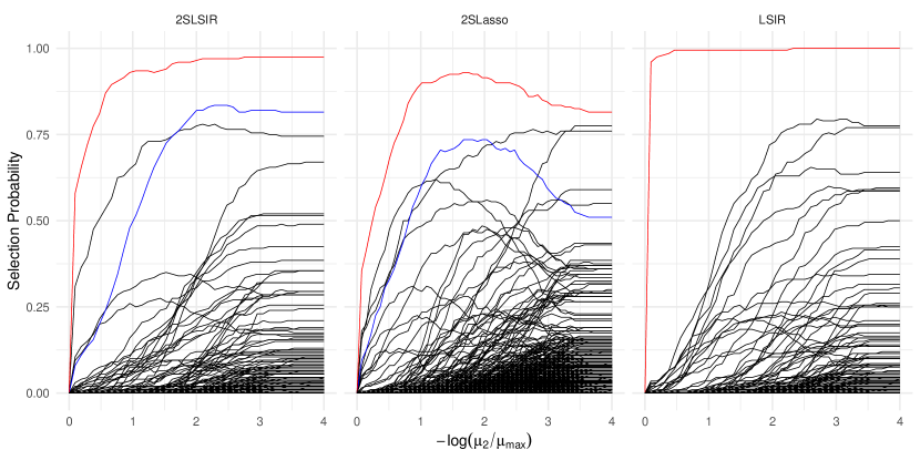
To select the number of structural dimensions , we used -means clustering of the (normalized) eigenvalues of the estimated matrix similar to that of Lin et al., (2019), with 2SLSIR and 2SLasso both selecting . Next, for each of the three estimators, we applied stability selection to compute the empirical selection probability (Meinshausen and Bühlmann,, 2010) for each gene over 100 random subsamples of size at each value of the tuning parameter. The upper bound for the per-family error rate was one while the selection cutoff was set to , meaning up to 75% number of components can be included in the estimates in each subsample. The results in Figure 1 present the selection path for each gene as a function of the second-stage tuning parameter . With the maximum selection probability across all the tuning parameters set to , LSIR selected seven genes, 2SLasso selected nine genes, while the proposed 2SLSIR selected six genes. Only one gene was chosen with a very high selection probability across all the three methods, while one additional gene is commonly selected by 2SLSIR and 2SLasso.
To further interpret the biological consequences of the selected genes, we conducted a Gene Ontology (GO) enrichment analysis for the genes chosen by each method. By annotating these genes for their participation in gene ontology, this analysis aims to identify which biological functions, known as GO terms, are over-represented in the selected genes (Bleazard et al.,, 2015). This over-representation is measured by the -values, adjusted for multiple comparisons, of the null hypothesis that this gene set is randomly associated with the GO, so a smaller (larger) -value indicates a more significant biological function. Furthermore, the gene ontology is divided into three main groups: biological processes (BP), molecular function (MF), and cellular component (CC). Figure 2 indicates that all the three methods capture a strong association between the obesity and lipid-related processes, including lipid transport, metabolism, and regulation. The one-stage LSIR focuses on genes regulating lipid transport and metabolic processes (e.g., lipid transporter activity, monocarboxylic acid transport), linking BMI to lipid dynamics at the cellular level. By contrast, both the 2SLasso and 2SLSIR estimators emphasize plasma lipoprotein metabolism (e.g., plasma lipoprotein particle clearance, protein-lipid complex). However, while the former puts more emphasis on the interplay between lipid metabolism and immune regulation (e.g., immunoglobulin binding), the latter focuses more on lipid catabolism and extracellular lipid transport (e.g., extracellular matrix structural constituent, lipase activity).

6.2 Measurement error: NHANES data
The National Health and Nutrition Examination Survey (NHANES) survey aims to assess the health and nutritional status of individuals in the United States, tracking the evolution of this over time (Centers for Disease Control and Prevention,, 2018). During the 2009-2010 survey period, participants were interviewed and asked to provide their demographic background, nutritional habits, and to undertake a series of health examinations. To assess the nutritional habits of participants, dietary data were collected using two 24-hour recall interviews, wherein the participants self-reported the consumed amounts of a set of food items during the 24 hours before each interview. Based on these recalls, daily aggregated consumption of water, food energy, and other nutrition components such as total fat and total sugar consumption were computed. In this section, we revisit the data application in Nghiem et al., 2023a , seeking to understand the relationship between total cholesterol level () for women and their long-term intakes of nutrition components, particularly a linear combination/s of these components carrying the full regression information, and whether these combinations are sparse in nature.
Let denote the vector of 42 nutritional covariates at the th interview for . Dietary recall data are well-known to be subject to measurement errors, so we assume , where represents the th latent long-term nutritional intake, and denotes an independent additive measurement error term following a multivariate Gaussian distribution with zero mean and covariance . We used an instrumental variable approach to account for this measurement error. Specifically, following Carroll et al., (Section 6.5.1, 2006) we treated the first replicate as a surrogate for and the second replicate as an instrument. Note in this case, the number of instruments . We then applied the linear instrumental variable model where is allowed to be a column-sparse matrix. It follows that we can write where . We then applied the proposed 2SLSIR estimator with the true covariate matrix replaced by the matrix , where we selected as the structural dimension following Nghiem et al., 2023a .
We first examined the estimated matrix coefficients from the first stage of the 2SLSIR estimation procedure. Figure S1 in the Supplementary Materials shows that the biggest element in each column of is typically the diagonal element, so the most important instrument to model the consumption of any dietary component in the second interview is, unsurprisingly, the consumption of the same component in the first interview. Overall, each column of is relatively sparse, with the number of non-zero coefficients in each column ranging from 3 to 20.
Next, we applied the same stability selection approach as in Section 6.1 to the 2SLSIR estimator and compared the resulting paths with the LSIR and 2SLasso estimators. With the maximum selection probability across all the tuning parameters being at least 0.5, LSIR selected five nutritional covariates, 2SLasso selected five covariates, while the proposed 2SLSIR selected six covariates. Figure 3 presents the selection path as a function of the tuning parameter for each nutrition component. The two components commonly selected by all the three methods were vitamin D and vitamin K, while both 2SLSIR and 2SLasso additionally select one more common component in folic acid. Vitamin D is the component with the largest estimated coefficients in both the 2SLSIR and 2SLasso estimators, and was the second largest in the LSIR estimator.

7 Discussion
In this paper, we propose an innovative two-stage Lasso SIR method to perform simultaneous sufficient dimension reduction and variable selection when endogeneity is present. We establish theoretical bounds for estimation and selection consistency of the proposed estimator, allowing the dimensionality of both the covariates and instruments to grow exponentially with sample size. Our simulation studies demonstrate that the 2SLSIR estimator exhibits superior performance compared with the one-stage Lasso SIR method that ignores endogeneity, and the two-stage Lasso method, that ignores non-linearity in the outcome model. We apply the proposed method in two data applications where endogeneity is well-known to be present, one in nutrition and one in statistical genomics.
Future research can extend the proposed two-stage Lasso SIR method to accommodate a possible non-linear relationship between the covariates and the instruments in the first stage. Different sparsity structures on the coefficient matrix , such as a low-rank matrix, can also be considered. One can also examine endogeneity in other sufficient dimension reduction methods, such as inverse regression models Cook and Forzani, (2008); Bura et al., (2022). Finally, the methods can be adapted to more complex settings, such as clustered or longitudinal data, for example as in (Nghiem and Hui,, 2024).
Acknowledgments
This work was supported by the Australian Research Council Discovery Project Grant DP230101908. Thanks to Shila Ghazanfar for useful discussions regarding the mouse obesity data application.
References
- Angrist and Krueger, (2001) Angrist, J. D. and Krueger, A. B. (2001). Instrumental variables and the search for identification: From supply and demand to natural experiments. Journal of Economic Perspectives, 15(4):69–85.
- Banerjee et al., (2014) Banerjee, A., Chen, S., Fazayeli, F., and Sivakumar, V. (2014). Estimation with norm regularization. In Ghahramani, Z., Welling, M., Cortes, C., Lawrence, N., and Weinberger, K., editors, Advances in Neural Information Processing Systems, volume 27. Curran Associates, Inc.
- Belloni et al., (2012) Belloni, A., Chen, D., Chernozhukov, V., and Hansen, C. (2012). Sparse models and methods for optimal instruments with an application to eminent domain. Econometrica, 80(6):2369–2429.
- Bleazard et al., (2015) Bleazard, T., Lamb, J. A., and Griffiths-Jones, S. (2015). Bias in microrna functional enrichment analysis. Bioinformatics, 31(10):1592–1598.
- Bura et al., (2022) Bura, E., Forzani, L., Arancibia, R. G., Llop, P., and Tomassi, D. (2022). Sufficient reductions in regression with mixed predictors. Journal of Machine Learning Research, 23(102):1–47.
- Caner, (2009) Caner, M. (2009). Lasso-type GMM estimator. Econometric Theory, 25(1):270–290.
- Caner et al., (2018) Caner, M., Han, X., and Lee, Y. (2018). Adaptive elastic net GMM estimation with many invalid moment conditions: Simultaneous model and moment selection. Journal of Business & Economic Statistics, 36(1):24–46.
- Card, (1999) Card, D. (1999). The causal effect of education on earnings. Handbook of Labor Economics, 3:1801–1863.
- Carroll et al., (2006) Carroll, R. J., Ruppert, D., and Stefanski, L. A. (2006). Measurement error in nonlinear models, volume 105. CRC press.
- Centers for Disease Control and Prevention, (2018) Centers for Disease Control and Prevention (2018). National health and nutrition examination survey data. https://wwwn.cdc.gov/nchs/nhanes/continuousnhanes/default.aspx?BeginYear=2009.
- Chernozhukov et al., (2015) Chernozhukov, V., Hansen, C., and Spindler, M. (2015). Post-selection and post-regularization inference in linear models with many controls and instruments. American Economic Review, 105(5):486–490.
- Cook and Forzani, (2008) Cook, R. D. and Forzani, L. (2008). Principal fitted components for dimension reduction in regression. Statistical Science, 23(4):485 – 501.
- Dai et al., (2024) Dai, S., Wu, P., and Yu, Z. (2024). New forest-based approaches for sufficient dimension reduction. Statistics and Computing, 34(5):176.
- Fan and Liao, (2014) Fan, J. and Liao, Y. (2014). Endogeneity in high dimensions. Annals of Statistics, 42(3):872.
- Friedman et al., (2010) Friedman, J., Hastie, T., and Tibshirani, R. (2010). Regularization paths for generalized linear models via coordinate descent. Journal of Statistical Software, 33:1–22.
- Gao et al., (2020) Gao, J., Kim, N., and Saart, P. W. (2020). On endogeneity and shape invariance in extended partially linear single index models. Econometric Reviews, 39(4):415–435.
- Hansen et al., (2008) Hansen, C., Hausman, J., and Newey, W. (2008). Estimation with many instrumental variables. Journal of Business & Economic Statistics, 26(4):398–422.
- Horn and Johnson, (2012) Horn, R. A. and Johnson, C. R. (2012). Matrix analysis. Cambridge university press.
- Hsing and Carroll, (1992) Hsing, T. and Carroll, R. J. (1992). An asymptotic theory for sliced inverse regression. The Annals of Statistics, pages 1040–1061.
- Hu et al., (2015) Hu, Y., Shiu, J.-L., and Woutersen, T. (2015). Identification and estimation of single-index models with measurement error and endogeneity. The Econometrics Journal, 18(3):347–362.
- Li, (2018) Li, B. (2018). Sufficient dimension reduction: Methods and applications with R. CRC Press, Florida.
- Li et al., (2017) Li, J., Cheng, K., Wang, S., Morstatter, F., Trevino, R. P., Tang, J., and Liu, H. (2017). Feature selection: A data perspective. ACM computing surveys (CSUR), 50(6):1–45.
- Li, (1991) Li, K.-C. (1991). Sliced inverse regression for dimension reduction. Journal of the American Statistical Association, 86:316–327.
- Lin et al., (2018) Lin, Q., Zhao, Z., and Liu, J. S. (2018). On consistency and sparsity for sliced inverse regression in high dimensions. The Annals of Statistics, 46:580–610.
- Lin et al., (2019) Lin, Q., Zhao, Z., and Liu, J. S. (2019). Sparse sliced inverse regression via lasso. Journal of the American Statistical Association, 114(528):1726–1739.
- Lin et al., (2015) Lin, W., Feng, R., and Li, H. (2015). Regularization methods for high-dimensional instrumental variables regression with an application to genetical genomics. Journal of the American Statistical Association, 110(509):270–288.
- Ma and Zhu, (2013) Ma, Y. and Zhu, L. (2013). A review on dimension reduction. International Statistical Review, 81:134–150.
- Meinshausen and Bühlmann, (2010) Meinshausen, N. and Bühlmann, P. (2010). Stability selection. Journal of the Royal Statistical Society Series B: Statistical Methodology, 72(4):417–473.
- Nghiem and Hui, (2024) Nghiem, L. H. and Hui, F. K. C. (2024). Random effects model-based sufficient dimension reduction for independent clustered data. Journal of Americal Statistical Association, Accepted for publication.
- (30) Nghiem, L. H., Hui, F. K. C., Muller, S., and Welsh, A. H. (2023a). Likelihood-based surrogate dimension reduction. Statistics and Computing, 34(1):51.
- (31) Nghiem, L. H., Hui, F. K. C., Müller, S., and Welsh, A. H. (2023b). Screening methods for linear errors-in-variables models in high dimensions. Biometrics, 79(2):926–939.
- (32) Nghiem, L. H., Hui, F. K. C., Müller, S., and Welsh, A. H. (2023c). Sparse sliced inverse regression via cholesky matrix penalization. Statistica Sinica, 33:1–33.
- Ravikumar et al., (2011) Ravikumar, P., Wainwright, M. J., Raskutti, G., and Yu, B. (2011). High-dimensional covariance estimation by minimizing -penalized log-determinant divergence. Electronic Journal of Statistics, 5.
- Sheng and Yin, (2016) Sheng, W. and Yin, X. (2016). Sufficient dimension reduction via distance covariance. Journal of Computational and Graphical Statistics, 25(1):91–104.
- Tan et al., (2018) Tan, K. M., Wang, Z., Zhang, T., Liu, H., and Cook, R. D. (2018). A convex formulation for high-dimensional sparse sliced inverse regression. Biometrika, 105(4):769–782.
- Wainwright, (2019) Wainwright, M. J. (2019). High-dimensional statistics: A non-asymptotic viewpoint, volume 48. Cambridge University Press.
- Wang et al., (2006) Wang, S., Yehya, N., Schadt, E. E., Wang, H., Drake, T. A., and Lusis, A. J. (2006). Genetic and genomic analysis of a fat mass trait with complex inheritance reveals marked sex specificity. PLoS Genetics, 2(2):e15.
- Windmeijer et al., (2019) Windmeijer, F., Farbmacher, H., Davies, N., and Davey Smith, G. (2019). On the use of the lasso for instrumental variables estimation with some invalid instruments. Journal of the American Statistical Association, 114(527):1339–1350.
- Xia et al., (2002) Xia, Y., Tong, H., Li, W., and Zhu, L.-X. (2002). An adaptive estimation of dimension reduction space. Journal of the Royal Statistical Society Series B, 64:363–410.
- Xu et al., (2022) Xu, K., Zhu, L., and Fan, J. (2022). Distributed sufficient dimension reduction for heterogeneous massive data. Statistica Sinica, 32:2455–2476.
- Yang, (1977) Yang, S.-S. (1977). General distribution theory of the concomitants of order statistics. The Annals of Statistics, pages 996–1002.
- Zhou and Zhu, (2016) Zhou, J. and Zhu, L. (2016). Principal minimax support vector machine for sufficient dimension reduction with contaminated data. Computational Statistics & Data Analysis, 94:33–48.
- Zhu et al., (2006) Zhu, L., Miao, B., and Peng, H. (2006). On sliced inverse regression with high-dimensional covariates. Journal of the American Statistical Association, 101(474):630–643.
- Zou, (2006) Zou, H. (2006). The adaptive lasso and its oracle properties. Journal of the American Statistical Association, 101:1418–1429.
Supplementary Materials
S1 Performance of Lasso SIR under endogenity
In this subsection, we consider a simple setting to demonstrate the performance of Lasso SIR when endogeneity is present. Suppose the random vector has the multivariate Gaussian distribution with zero mean, marginal covariance matrix , and the marginal variance . In this case, it follows that
| (12) |
where is the correlation between and . Furthermore, assume that the outcome is generated from a linear model Then we have
and, as a result,
so the eigenvector of is the normalized eigenvector of .
To demonstrate the performance of Lasso SIR, we conducted a small simulation study where we set and , so the target of estimation for Lasso SIR is both the column space of as well as its support set . We generated from the multivariate Gaussian distribution (12), with three scenarios for the correlation vector , including (I) , (II) , and (III) . We then simulated the outcome from either the linear model or the non-linear model . We varied and for each simulation configuration, we generated samples.
For each generated sample, we computed the Lasso SIR estimator with the tuning parameter selected by 10-fold cross-validation, as implemented by the LassoSIR package. We reported the estimation error in estimating the column space spanned by , as measured by . For variable selection performance, we computed the area under the receiver operating curve (AUC); an AUC of one indicates a clear separation between the estimates of non-important variables and the those of important variables in .
Table S3 shows that the performance of the Lasso SIR estimator aligns with our theoretical results. In the first case, the correlation vector is proportional to the true , so the Lasso SIR maintains both estimation and variable selection consistency, as evidenced by a decreasing estimation error when increases and an AUC of 1. In the second case, the Lasso SIR estimator gives a consistent estimate of the space spanned by , which has a different direction but the same support compared to the true . Hence, the Lasso SIR is not estimation consistent, but still has an AUC of 1. In the last case, the Lasso SIR estimator gives a consistent estimate for the space spanned by , which has both a different direction and a different support from those of the true . As a result, the Lasso SIR estimator is not selection or estimation consistent.
| Linear link | Sine link | ||||
|---|---|---|---|---|---|
| Error | AUC | Error | AUC | ||
| (I) | 100 | 0.095 | 1.000 | 0.876 | 0.853 |
| 500 | 0.039 | 1.000 | 0.402 | 0.992 | |
| 1000 | 0.028 | 1.000 | 0.258 | 1.000 | |
| (II) | 100 | 0.659 | 1.000 | 0.768 | 0.907 |
| 500 | 0.643 | 1.000 | 0.674 | 0.995 | |
| 1000 | 0.639 | 1.000 | 0.661 | 1.000 | |
| (III) | 100 | 1.001 | 0.758 | 1.003 | 0.739 |
| 500 | 1.000 | 0.744 | 0.999 | 0.756 | |
| 1000 | 1.000 | 0.728 | 0.999 | 0.747 | |
S2 Proofs
S2.1 Proof of Proposition 1
Without loss of generality, assume the expectation of , the marginal covariance matrix , and the marginal variance . In this case, it follows that
By the law of iterated expectation, we have
Next, by the property of the multivariate Gaussian distribution we obtain
which is in the subspace spanned by if and only if can be written in the form for a matrix , i.e .
S2.2 Proof of Proposition 2
Let , so each element of always has the same sign as that of . Let . Since is fixed, the cross product with probability one for all . As a result, we have with probability one.
From the definition of the Lasso-SIR estimator and writing , we have
Equivalently, we have
By construction, we have , the eigenvector associated with the th largest eigenvalue of . By the law of large numbers, we have , so . Furthermore, as , we have so . Therefore, as . the vector satisfies
Since and , we have , so as .
S2.3 Proof of Lemma 1
The instrument is independent of both and , so the conditional expectation is also independent of both and . By the properties of conditional expectation, we have
| (since and are independent) | ||||
where step follows from Condition 3.1 in the main text and Lemma 1.01 of Li, (2018). The last equation shows that the conditional expectation of is contained in the space spanned by , and the required result follows.
S2.4 Proof of Lemma 2
Recall and are the eigenvectors associated with and , respectively. Hence, maximizes the function subject to , and
Equivalently, we have and, where for two matrices and , we let be their dot product. Writing , we obtain
| (13) |
For the left hand side of (13), since and , then we have .
Turning to the right hand side of (13), applying Hölder’s inequality we obtain
where for any matrix , we let denote its elementwise maximum norm, and the second inequality above follows from . Section S2.5 studies the properties of ; in particular, it establishes that there exist positive constants and such that
with probability at least . With the same probability then, we obtain
as required.
S2.5 Properties of
The developments below follow closely the work of Tan et al., (2018). Note
where . Similarly, we can write , with
| (14) |
with , being the vector of ones, and denoting the identity matrix. Define , and let , and .
We now bound the elementwise maximum norm . By the triangle inequality, for any , we have
| (15) | ||||
From Theorem 1 in the main text we have with probability at least for any . Furthermore by Condition 4.2 in the main text, we have and . Therefore, obtain
| (16) |
For the second term , by the triangle inequality we have that
with probability at least , assuming . Next, Lemma 4 provides an upper bound on as follows.
Lemma 4.
Under the Conditions 4.1-4.5 in the main text, we have with probability at least .
The proof for Lemma 4and other technical results in this section are deferred to section S3. Combining Lemma 1 and union bound then, we obtain
| (17) |
with a probability at least .
Finally for the term , by the triangle inequality we also have
with a probability at least , assuming . Hence, with a probability of at least , we have
| (18) |
S2.6 Proof of Lemma 3
By the optimality of , we obtain
| (20) |
Letting and substituting into (20), we obtain
Expanding the square, cancelling the same terms on both sides, and rearranging terms, we have
| (21) |
By definition, we have , and so (21) is equivalent to
Applying Hölder’s inequality and the condition on from the Lemma, we obtain
It follows that
| (22) |
Furthermore, applying the (reverse) triangle inequality gives
Since , then equation (22) further leads to
It follows from step (iv) that , or .
Next, we apply the following result which establishes the sample covariance matrix satisfies the RE condition with a parameter with high probability.
Proposition 3.
Assume Conditions 4.1-4.2, 4.5 and the requirements of Theorem 1 are satisfied. Then there exists a constant such that , for any , with probability at least , for constants and .
Conditioned on this RE condition, step (v) implies
As a result, we obtain
as required.
S2.7 Proof of Theorem 2
Recall that with . By Lemma 2, the term is non-zero with high probability. Hence, with the same probability. Next, by the Cauchy-Schwartz inequality we have
Thus the required result will follow from Lemma 3.2, if the choice of as given in theorem satisfies with probability tending to one. It remains then to find an upper bound for .
By the triangle inequality, we have
| (23) |
We will upper bound each term on the right-hand side of (23). For the first term, note by definition, i.e., the eigenvector associated with the largest eigenvalue of . Hence, we obtain
for a large positive constant , where step (i) above follows since
and step (ii) follows from applying Lemma 2.
S2.8 Proof of Theorem 3
The proof of this theorem has the same steps as the primal-dual witness technique, which are used in the proof for variable selection consistency of the Lasso estimator in the regular linear model (see Section 7.5.2, Wainwright,, 2019), as well as in the two-stage Lasso estimator of Lin et al., (2015). In our context, the proposed two-stage Lasso SIR estimator is the minimizer of
Applying the Karush–Kuhn-Tucker optimality condition, the estimator has to satisfy
| (25) |
and
| (26) |
It suffices to find a solution such that both (25) and (26) hold. To achieve this, the idea of the primal-dual witness technique is first let , then construct from (25), and finally show that the obtained satisfies (26). Central to this development is the following lemma regarding the bound of the sample covariance .
Lemma 5.
Assume Condition 4.7 is satisfied. If there exists a constant such that
| (27) |
then with probability at least , the matrix , where is defined from the first stage with the tuning parameters as stated in Theorem 1, satisfies
| (28) |
Using a similar argument as in the proof of Theorem 2, there also exist constants and such that
| (29) |
with probability at least . Hence, we will condition on both events (28) and (29) in the remaining part of the proof.
Next, recall , and by definition of we have , which is the eigenvector associated with the largest eigenvalue of . Since , then (25) is equivalent to
where is defined previously. Hence, we obtain
| (30) |
and therefore
| (31) |
Substituting (28) and (29) into (31), we obtain
where the last step follows from
and by the choice of as stated in the theorem. Thus we have , and since by construction then we have .
S2.9 Proof of Theorem 4
Consider the multiple index model with . In this case, the quantities and are the semi-orthogonal matrices of eigenvectors of and , respectively. Let be the projection of on . By Lemma 1, we have where is a non-zero diagonal matrix, such that . Hence, we can write
where . When is a invertible matrix, the column space spanned by and that spanned by are the same, and so are the index sets for their non-zero rows.
Proposition 4 establishes a lower bound on the trace of .
Proposition 4.
Assume Conditions 4.1–4.6 are satisfied. Then there exist positive constants , , and such that
with probability at least .
Furthermore, by the Cauchy-Schwartz inequality, we have . By Condition 4.3 with and Condition 4.4 with , we thus have with a probability at least . This implies that with the same probability, the matrix is invertible.
Conditioning on the invertibility of , Lemma 3 holds for each column . As a result, we have
for any . Hence, by a similar argument to the proof of Theorem 2, and with the choice of as stated in the theorem, there exist constants , and such that
with probability at least .
Finally, turning to variable selection consistency, let and . By a similar argument to that in the proof of Theorem 3, under the condition on as stated in Theorem 4, we have for with probability at least . Note the diagonal element of the estimated projection matrix if and only if all one across . Hence, taking the union bound, we have with a probability at least .
S3 Additional derivations
S3.1 Proof of Lemma 4
By the triangle inequality, we have
Also, by the property of sub-Gaussian random variables, there exist positive constants and such that
| (32) |
with probability at least (Ravikumar et al.,, 2011; Tan et al.,, 2018). Next, we will bound the elementwise maximum norm
Following Zhu et al., (2006), we introduce the following notations. Let denote the order statistics of the outcome data , and be the concomitants in the data. Define and , and let be the matrix whose th row is and be the matrix whose th row is . Note we have and for all .
Let , and be the th element of , and , respectively, for . Similar to Proposition 2 in the Supplementary Materials of Tan et al., (2018), we obtain the following properties of and , whose proof is omitted.
Proposition 5.
Under Condition 4.1, , and are sub-Gaussian with sub-Gaussian norms , and , respectively, for .
Noting and using the same decomposition as in Zhu et al., (2006), write
| (33) | ||||
where denotes the Kronecker product, , , and is the vector of ones. By the triangle inequality, we obtain
| (34) |
We proceed by bounding each term on the right hand side of (34).
For the first term , noting that , then . On combining this with Proposition 5, it follows that each element of is a centered sub-exponential random variable with sub-exponential norm bounded by , since by condition 1. Therefore, with probability at least , we have
| (35) |
For term , we note that has all diagonal elements zero and off-diagonal elements , so each element of is the sum of terms of the form with (note and can be the same). Next, conditional on the order statistics , the quantities and are independent (Yang,, 1977). On combining this with Proposition 5, we have that is zero-mean sub-exponential with sub-exponential norm bounded by . Therefore, with probability at least , we have
| (36) |
Next, we consider the term , where it suffices to consider the term . Let denote the matrix whose th row is given by for , and whose th row is . It is straightforward to see that and , where for any , we have
Hence, by the property of the Kronecker product, we obtain
We have , where all are sub-Gaussian random variables by Proposition 5 for all and . Therefore, with probability at least , we have that . Also note that in the matrix , all the columns of have their sum of absolute values less than two, i.e . On combining these results, we obtain
where the last inequality follows from condition 4.6. Therefore, with probability at least , we obtain
| (37) |
Finally, we consider the term . Substituting and using properties of Kronecker products, we have
Since all the elements of have absolute value less than , then
| (38) |
where the last inequality follows from Condition 4.6.
S3.2 Proof of Proposition 3
Let . Then we have
| (40) |
where the last inequality follows from Condition 4.5 on the restricted eigenvalue of . Next, we provide an upper bound on the second term. We have
Since , i.e , then we obtain . Furthermore, noting that and , then we have
By the triangle inequality, we obtain
| (41) | ||||
The three terms , and are similar to and in Section S2.5 with and replaced by and , respectively. It follows that by a similar argument, we obtain
| (42) |
with probability at least .
Substituting the above into (40) and under the assumption , then there exists a positive constant such that
with probability at least , as required.
S3.3 Proof of Lemma 28
From equation (42) in the proof of Proposition 3, with probability at least we have
Conditioning on this event, and combining it with (27), we obtain
and similarly,
Next, by an error bound for matrix inversion (Horn and Johnson,, 2012, Section 5.8), we obtain
Applying the triangle inequality, we have
which proves the first inequality in (28).
To show the second inequality, we can write
It follows that
as required.
S3.4 Proof of Proposition 4
The proof of this proposition generalizes the proof of Lemma 2 above. By the variational definition of eigenvectors, maximizes subject to , and so
or equivalently , where for two matrices and we let denote their dot product. Writing , it follows that
| (43) |
For the left-hand side of (43), by an eigendecomposition we have and . It follows that
S4 Additional simulation results
| Model | Error | F1 | ||||||||
|---|---|---|---|---|---|---|---|---|---|---|
| LSIR | 2SLasso | 2SLSIR | LSIR | 2SLasso | 2SLSIR | |||||
| 500 | (i) | Strong | 0.28 (0.07) | 1.05 (0.22) | 0.13 (0.04) | 0.99 (0.03) | 0.52 (0.18) | 1.00 (0.00) | ||
| Weak | 0.37 (0.08) | 1.01 (0.24) | 0.18 (0.06) | 0.96 (0.07) | 0.54 (0.18) | 0.99 (0.03) | ||||
| Mixed | 0.29 (0.08) | 1.04 (0.20) | 0.11 (0.03) | 0.98 (0.05) | 0.57 (0.18) | 1.00 (0.00) | ||||
| (ii) | Strong | 0.26 (0.08) | 0.24 (0.07) | 0.13 (0.05) | 1.00 (0.02) | 0.98 (0.04) | 1.00 (0.00) | |||
| Weak | 0.35 (0.07) | 0.31 (0.08) | 0.18 (0.07) | 0.97 (0.05) | 0.94 (0.08) | 1.00 (0.01) | ||||
| Mixed | 0.30 (0.06) | 0.24 (0.08) | 0.11 (0.04) | 0.99 (0.03) | 0.98 (0.05) | 1.00 (0.00) | ||||
| 1000 | (i) | Strong | 0.30 (0.07) | 0.98 (0.22) | 0.09 (0.03) | 0.99 (0.03) | 0.57 (0.18) | 1.00 (0.00) | ||
| Weak | 0.38 (0.07) | 0.90 (0.23) | 0.13 (0.04) | 0.96 (0.06) | 0.63 (0.16) | 1.00 (0.01) | ||||
| Mixed | 0.35 (0.06) | 0.89 (0.24) | 0.06 (0.02) | 0.97 (0.07) | 0.63 (0.17) | 1.00 (0.00) | ||||
| (ii) | Strong | 0.31 (0.07) | 0.18 (0.05) | 0.09 (0.03) | 0.99 (0.04) | 1.00 (0.02) | 1.00 (0.00) | |||
| Weak | 0.39 (0.07) | 0.22 (0.07) | 0.12 (0.04) | 0.94 (0.08) | 0.98 (0.05) | 1.00 (0.01) | ||||
| Mixed | 0.34 (0.06) | 0.16 (0.05) | 0.07 (0.02) | 0.97 (0.07) | 1.00 (0.01) | 1.00 (0.00) | ||||
| Model | Error | F1 | |||||||
|---|---|---|---|---|---|---|---|---|---|
| LSIR | 2SLSIR | LSIR | 2SLSIR | ||||||
| 500 | (iii) | Strong | 0.88 (0.23) | 0.67 (0.26) | 0.61 (0.16) | 0.73 (0.16) | |||
| Weak | 1.02 (0.21) | 0.92 (0.29) | 0.56 (0.12) | 0.62 (0.17) | |||||
| Mixed | 0.98 (0.19) | 0.70 (0.26) | 0.49 (0.11) | 0.70 (0.16) | |||||
| (iv) | Strong | 0.40 (0.21) | 0.40 (0.24) | 0.93 (0.11) | 0.93 (0.13) | ||||
| Weak | 0.50 (0.20) | 0.49 (0.25) | 0.88 (0.13) | 0.85 (0.15) | |||||
| Mixed | 0.43 (0.21) | 0.39 (0.23) | 0.88 (0.14) | 0.91 (0.14) | |||||
| 1000 | (iii) | Strong | 0.97 (0.21) | 0.49 (0.29) | 0.55 (0.13) | 0.86 (0.15) | |||
| Weak | 1.08 (0.20) | 0.66 (0.29) | 0.53 (0.10) | 0.73 (0.18) | |||||
| Mixed | 1.05 (0.16) | 0.50 (0.28) | 0.45 (0.07) | 0.84 (0.14) | |||||
| (iv) | Strong | 0.38 (0.21) | 0.31 (0.24) | 0.95 (0.13) | 0.97 (0.11) | ||||
| Weak | 0.49 (0.22) | 0.35 (0.24) | 0.88 (0.15) | 0.93 (0.13) | |||||
| Mixed | 0.43 (0.22) | 0.29 (0.22) | 0.88 (0.16) | 0.96 (0.12) | |||||
S5 Additional results for the application
