High-dimensional inference for single-index model with latent factors
Abstract
Models with latent factors recently attract a lot of attention. However, most investigations focus on linear regression models and thus cannot capture nonlinearity. To address this issue, we propose a novel Factor Augmented Single-Index Model. We first address the concern whether it is necessary to consider the augmented part by introducing a score-type test statistic. Compared with previous test statistics, our proposed test statistic does not need to estimate the high-dimensional regression coefficients, nor high-dimensional precision matrix, making it simpler in implementation. We also propose a Gaussian multiplier bootstrap to determine the critical value. The validity of our procedure is theoretically established under suitable conditions. We further investigate the penalized estimation of the regression model. With estimated latent factors, we establish the error bounds of the estimators. Lastly, we introduce debiased estimator and construct confidence interval for individual coefficient based on the asymptotic normality. No moment condition for the error term is imposed for our proposal. Thus our procedures work well when random error follows heavy-tailed distributions or when outliers are present. We demonstrate the finite sample performance of the proposed method through comprehensive numerical studies and its application to an FRED-MD macroeconomics dataset.
Keywords: Factor augmented regression, latent factor regression, robustness, single-index model, score-type test statistic
1 Introduction
The rapid advancement of information technology has brought significant changes in both data collection and analysis. Various disciplines, such as economics, social sciences, and genetics, increasingly collect high-dimensional data for comprehensive research and analysis (Belloni et al.,, 2012; Bühlmann et al.,, 2014; Fan et al.,, 2020). Most existing high-dimensional procedures (for a recent comprehensive review, see for instance Fan et al., (2020)) were conducted under the assumption that there are no latent factors associated with both the response variables and covariates. However, it is important to acknowledge that this assumption is often violated in real-world. For instance, in genetic studies, the influence of specific DNA segments on gene expression can be confounded by population structure and artifacts in microarray expression (Listgarten et al.,, 2010). Similarly, in healthcare research, disentangling the impact of nutrient intake on cancer risk can be confounded by factors such as physical health, social class, and behavioral aspects (Fewell et al.,, 2007). Failure to account for latent factors in the model may lead to biased inferences. These examples underscore the importance of considering latent factors within models to ensure accurate and reliable conclusions.
To tackle the issues posed by latent factors, Fan et al., (2024) proposed the following Factor Augmented sparse linear Regression Model (FARM):
| (1.1) | ||||
| (1.2) |
Here, is a response variable, is a -dimensional covariate vector, is a -dimensional vector of latent factors, is the corresponding factor loading matrix, and is a -dimensional vector of idiosyncratic components, which is uncorrelated with . The and are vectors of regression parameters quantifying the contribution of and , respectively. The random error satisfies that , and is independent of and . In fact, model (1.2) is a commonly used structure for characterizing the interdependence among features. In this framework, the variables are intercorrelated through a shared set of latent factors.
Numerous methodologies have been proposed to enable statistical analysis regarding models with latent factors. Guo et al., (2022) introduced a deconfounding approach for conducting statistical inference on individual regression coefficient , integrating the findings of Ćevid et al., (2020) with the debiased Lasso method (Zhang and Zhang,, 2014; Van de Geer et al.,, 2014). Ouyang et al., (2023) investigated the inference problem of generalized linear regression models (GLM) with latent factors. Sun et al., (2023) considered the multiple testing problem for GLM with latent factors. Bing et al., (2023) focused on inferring high-dimensional multivariate response regression models with latent factors.
Although the above FARM is powerful to deal with latent factors, it may be not flexible enough to handle the nonlinear relationship between covariates and the response. To capture the nonlinearity, the single-index model (SIM) is usually adopted due to its flexibility and interpretability. As a result, the SIM has been the subject of extensive attention and in-depth research in the past decade. Actually, several approaches have been explored for the variable selection problem in high-dimensional SIMs. Examples include Kong and Xia, (2007), Zhu and Zhu, (2009), Wang et al., (2012), Radchenko, (2015), Plan and Vershynin, (2016), and Rejchel and Bogdan, (2020). However, limited attention has been paid to discuss SIMs with latent factors. This motivates us to investigate the high-dimensional single-index model with latent factors.
To this end, we consider the following Factor Augmented sparse Single Index Model (FASIM), which integrates both the latent factors and the covariates,
| (1.3) |
Here the link function is unknown, and other variables and parameters in model (1) remain consistent with those defined in model (1.1). When , the above FASIM reduces to the FARM introduced by Fan et al., (2024). Since can be unknown, the above FASIM is very flexible and can capture the nonlinearity.
For the FASIM, the first concern is whether is zero or not. Actually if , the model reduces to a single-index factor regression model, which was also considered by Fan et al., (2017), Jiang et al., (2019), and Luo et al., (2022). For this important problem, Fan et al., (2024) considered the maximum of the debiased lasso estimator of under FARM. However, their procedure is computationally expensive since it requires to estimate high-dimensional regression coefficients and also high-dimensional precision matrix. In this paper, we first introduce a score-type test statistic, which does not need to estimate high-dimensional regression coefficients, nor high-dimensional precision matrix. Hence, our procedure is very simple in implementation. We also propose a Gaussian multiplier bootstrap to determine our test statistic’s critical value. The validity of our procedure is theoretically established under suitable conditions. We also give a power analysis for our test procedure.
When the FASIM is adequate, it is then of importance to estimate the parameters in FASIM. For the SIM, Rejchel and Bogdan, (2020) considered distribution function transformation of the responses, and then estimated the unknown parameters using the Lasso method. Similar procedures have also been investigated by Zhu and Zhu, (2009) and Wang et al., (2012). This enhances the model’s robustness in scenarios where random errors follow heavy-tailed distributions or when outliers are present. Motivated by their procedures, we also consider the distribution function transformation of the responses and then introduce penalized estimation of unknown parameters. However, it should be emphasized here, different from Zhu and Zhu, (2009), Wang et al., (2012) and Rejchel and Bogdan, (2020), in our model and are unobserved and must be estimated firstly. This would give additional technical difficulty. In this paper, we establish the estimation error bounds of our introduced penalized estimators under mild assumptions. Notably, no moment condition is required for the error term in the FASIM.
Lastly, we investigate the construction of confidence interval for each regression coefficient in the FASIM. Due to the inherent bias, the penalized estimator cannot be directly used in statistical inference. Eftekhari et al., (2021) investigated the inference problem of the SIM by adopting the debiasing technique (Zhang and Zhang,, 2014; Van de Geer et al.,, 2014). However, their procedure cannot handle latent factors. To this end, we introduce debiased estimator for the FASIM and also establish its corresponding asymptotic normality. Compared with Eftekhari et al., (2021), our procedure does not need sample-splitting and is robust to outliers.
The remainder of this paper is structured as follows. In Section 2, we delve into the reformulation of the FASIM and the estimation of the latent factors. In Section 3, we develop a powerful test procedure for testing whether . In Section 4, we consider the regularization estimation of and establish the and -estimation error bounds for this estimation. Further we introduce debiased estimator and construct confidence interval for each coefficient. We present the findings of our simulation studies in Section 5 and provide an analysis of real data in Section 6 to assess the performance and effectiveness of the proposed approach. Conclusions and discussions are presented in Section 7. Proofs of the main theorems are provided in the Appendix. Proofs of related technical Lemmas are attached in the Supplementary Material.
Notation. Let denote the indicator function. For a vector , we denote its norm as , , and . For any integer , we define . The Orlicz norm of a scalar random variable is defined as . For a random vector , we define its Orlicz norm as . Furthermore, we use , and to denote the identity matrix in , a vector of dimensional with all elements being and all elements being , respectively. For a matrix , represents the -th row of , and represents the -th column of . We define , , , and to be its Frobenius norm, element-wise max-norm, matrix -norm, matrix -norm and the element-wise sum-norm, respectively. Besides, we use and to denote the minimal and maximal eigenvalues of , respectively. We use to denote the cardinality of a set . For two positive sequences , , we write if there exists a positive constant such that , and we write if . Furthermore, if is satisfied, we write . If and , we write it as for short. In addition, and have similar meanings as above except that the relationship of holds with high probability. The parameters and appearing in this paper are all positive constants.
2 Factor augmented single-index model
In this section, we investigate the reformulation of the FASIM and the estimation of the latent factors, as well as their properties.
2.1 Reformulation of FASIM
The unknown smooth function makes the estimation of the FASIM challenging. To address this concern, we reformulate the FASIM as a linear regression model with transfomed response. With this transformation, we estimate the parameters avoiding estimating the unknown function .
Without loss of generality, we assume that , and is a positive definite matrix. Let and for a given transformation function of the response. Define , , , and . In the context of the SIM framework, the following linear expectation condition is commonly assumed.
Proposition 2.1.
Assume that is a linear function of . Then is proportional to , that is for some constant .
Proposition 2.1 is from Theorem 2.1 of Li and Duan, (1989). The condition in this proposition is referred to as the linearity condition (LC) for predictors. It is satisfied when follows an elliptical distribution, a commonly used assumption in the sufficient dimension reduction literature (Li,, 1991; Cook and Ni,, 2005). Hall and Li, (1993) showed that the LC holds approximately to many high-dimensional settings. Throughout the paper, we assume , which is a relatively mild assumption. In fact, when is monotone and is monotonic with respect to the first argument, this assumption is anatomically satisfied.
Following from the definition of and , our model can be rewritten as:
| (2.1) |
where , and the error term satisfies , and . This implies that we now recast the FASIM as a FARM with transformed response. Actually for identification of the FASIM, it is usually assumed that and its first element is positive. Thus the estimation of the direction of is sufficient for the FASIM. The proportionality between and , along with the previous mentioned transformed linear regression model (2.1), reduces the difficulty of analysis.
In practice, we need to choose an appropriate transformation function . It’s worth mentioning that the procedure in Eftekhari et al., (2021) essentially works with . Motivated by Zhu and Zhu, (2009) and Rejchel and Bogdan, (2020), we set , where is the distribution function of . This specific choice could make our procedures be robust against outliers and heavy tails. Actually with equation (2.1), given the widely imposed sub-Gaussian assumption on the predictors, the boundedness of would lead the transformed error term being sub-Gaussian, even if the original error term comes from Cauchy distribution. The response-distribution transformation is preferred due to some additional reasons which will be discussed later.
2.2 Factor estimation
Throughout the paper, we assume that the data are independent and identically distributed (i.i.d.) copies of . Let , , and . We consider the high-dimensional scenario where the dimension of the observed covariate vector can be much larger than the sample size . For the FASIM, we first need to estimate the latent factor vector since only the predictor vector and the response are observable. To address this issue, we impose an identifiability assumption similar to that in Fan et al., (2013). That is
Consequently, the constrained least squares estimator of based on is given as
| (2.2) | ||||
| subjectto |
Let , with . Denote .
Elementary manipulation yields that the columns of are the eigenvectors corresponding to the largest eigenvalues of the matrix and . Then the estimator of is
see Fan et al., (2013). Since is related to the number of spiked eigenvalues of , it is usually small. Therefore, we treat as a fixed constant as suggested by Fan et al., (2024). Additionally, let , and be suitable estimators of the covariance matrix of , the matrix consisting of its leading eigenvalues and the matrix consisting of their corresponding orthonormalized eigenvectors , respectively.
We proceed by presenting the regularity assumptions imposed in seminal works about factor analysis, such as Bai, (2003) and Fan et al., (2013, 2024).
Assumption 1.
We make the following assumptions.
-
(i)
There exists a positive constant such that and . In addition, .
-
(ii)
There exists a constant such that .
-
(iii)
There exists a constant such that and
-
(iv)
There exists a positive constant such that , , and .
Assumption 2.
(Initial pilot estimators). Assume that , and satisfy , , and .
Remark 1.
Assumption 2 is taken from Bayle and Fan, (2022). This assumption holds in various scenarios of interest, such as for the sample covariance matrix under sub-Gaussian distributions (Fan et al.,, 2013). Moreover, the estimators like the marginal and spatial Kendall’s tau (Fan et al.,, 2018), and the elementwise adaptive Huber estimator (Fan et al.,, 2019) satisfy this assumption.
We summarize the theoretical results related to consistent factor estimation in Lemma 1 in Supplementary Material, which directly follows from Proposition 2.1 in Fan et al., (2024) and Lemma 3.1 in Bayle and Fan, (2022).
In practice, the number of latent factors is often unknown, and determining in a data-driven way is a crucial challenge. Numerous methods have been introduced in the literature to estimate the value of (Bai and Ng,, 2002; Lam and Yao,, 2012; Ahn and Horenstein,, 2013; Fan et al.,, 2022). In this paper, we employ the ratio method for our numerical studies (Luo et al.,, 2009; Lam and Yao,, 2012; Ahn and Horenstein,, 2013). Let be the -th largest eigenvalue of . The number of factors can be consistently estimated by
where is a prescribed upper bound for . In our subsequent theoretical analysis, we treat as known. All the theoretical results remain valid conditioning on that is a consistent estimator of .
3 Adequacy test of factor model
In this section, we aim to assess the adequacy of the factor model and determining whether FASIM (1) can serve as an alternative to . The primary question of interest pertains to the following hypothesis:
| (3.1) |
From Proposition 2.1, the null hypothesis is also equivalent to .
3.1 Factor-adjusted score-type test
In this subsection, we develop a factor-adjusted score type test (FAST) and derive its Gaussian approximation result. For the adequacy testing problem, Fan et al., (2024) considered the maximum of the debiased lasso estimator of under FARM. However, their procedure requires to estimate high-dimensional regression coefficients and also high-dimensional precision matrix, and thus is computationally expensive. While our proposed FAST does not need to estimate high-dimensional regression coefficients, nor high-dimensional precision matrix. Hence, Our procedure is straightforward to implement, saving both computation time and computational resources.
Under the null hypothesis in (3.1), we have
While under alternative hypothesis , we have
This observation motivates us to consider the following individual test statistic
| (3.2) |
Here we utilize the empirical distribution as an estimator of . In the empirical distribution function, the term is the rank of . Since statistics with ranks such as Wilcoxon test and the Kruskall-Wallis ANOVA test, are well-known to be robust, this intuitively explains why our procedures with response-distribution transformation function would be robust with respect to outliers in response. We consider the least squares estimator . Denote . To test the null hypothesis , we consider norm of . That is,
| (3.3) |
It is clear that in the FAST statistic defined above, we only need to estimate a low-dimensional parameter , and no high-dimensional parameters are required. In addition, since FAST does not rely on the estimation of the precision matrix, we can avoid assumptions about the norm of the precision matrix, as demonstrated in Fan et al., (2024). Further define as follows:
| (3.4) |
where . Denote and . Let . It could be shown that .
Assumption 3.
.
The is bounded away from zero.
Assumption 3 is mild and frequently employed in high-dimensional settings, which is the technical requirement to bound the difference between and , where . Specifically, condition (i) imposes suitable restriction on the growth rate of and is commonly used in the high-dimensional inference literature, see Zhang and Cheng, (2017) and Dezeure et al., (2017). Condition (ii) imposes a boundedness restriction on the second moment of , which is also assumed in Ning and Liu, (2017).
Theorem 3.1.
Theorem 3.1 indicates that our test statistic can be approximated by the maximum of a high-dimensional Gaussian vector under mild conditions. Based on this, we can reject the null hypothesis at the significant level if and only if , where is the -th quantile of the distribution of .
As demonstrated by many authors, such as Cai et al., (2014) and Ma et al., (2021), the distribution of can be asymptotically approximated by the Gumbel distribution. However, this generally requires restrictions on the covariance matrix of . For instance, it requires that the eigenvalues of are uniformly bounded. In addition, the critical value obtained from the Gumbel distribution may not work well in practice since this weak convergence is typically slow (Zhang and Cheng,, 2017). Instead of adopting Gumbel distribution, we consider using bootstrap to approximate the distribution of .
3.2 Gaussian multiplier bootstrap
Given that is unknown, we employ the Gaussian multiplier bootstrap to derive the critical value . The procedures and theoretical properties of the Gaussian multiplier bootstrap are outlined in this subsection.
-
1.
Generate i.i.d. random variables independent of the observed dataset , and compute
(3.6) Here .
-
2.
Repeat the first step independently for times to obtain . Approximate the critical value via the -th quantile of the empirical distribution of the bootstrap statistics:
(3.7) -
3.
We reject the null hypothesis if and only if
(3.8)
Theorem 3.2.
Suppose that conditions in Theorem 3.1 are satisfied. Under the null hypothesis, we have
3.3 Power analysis
We next consider the asymptotic power analysis of the . To demonstrate the efficiency of the test statistic, we consider the following local alternative parameter family for under .
| (3.9) |
where is a positive constant. The quantifies the sparsity of the parameter . Denote .
Assumption 4.
Suppose that is a diagonal matrix and is bounded away from zero.
Assumption 4 outlines the diagonal structure of the covariance matrix , a common assumption in factor analysis (Kim and Mueller,, 1978). We should also note that this diagonality of is only imposed here for simplify the power analysis.
Theorem 3.3.
Theorem 3.3 suggests that our test procedure maintains high power even when only a few components of have magnitudes larger than . Thus, our testing procedure is powerful against sparse alternatives. Notably, this separation rate represents the minimax optimal rate for local alternative hypotheses, as discussed in Verzelen, (2012), Cai et al., (2014), Zhang and Cheng, (2017), and Ma et al., (2021).
4 Estimation and inference of FASIM
When the null hypothesis is rejected, indicating that the factor model is inadequate, we need to consider FASIM. In this section, we aim to investigate the estimation and inference of the FASIM.
4.1 Regularization estimation
In the high-dimensional regime, we employ penalty (Tibshirani,, 1996) to estimate the unknown parameter vectors and in model (2.1):
| (4.1) |
where is a tuning parameter.
By utilizing pseudo response observations instead of , our approach is inherently robust when confronting with outliers. We note that for the SIM without latent factors, the distribution function transformation has also been considered by many other authors, such as Zhu and Zhu, (2009), Wang et al., (2012), and Rejchel and Bogdan, (2020). However, in our model and are unobserved and must be estimated firstly. Thus we require additional efforts to derive the theoretical properties of .
Let represent the residuals of the response vector after it has been projected onto the column space of , where is the corresponding projection matrix. Since , . Then direct calculations yield that the solution of (4.1) is equivalent to
| (4.2) | ||||
| (4.3) |
For any vector defined in (4.2), we have the following result.
Based on the empirical distribution function of the response, we establish the and -error bounds for our introduced estimator in Theorem 4.1. Compared with Zhu and Zhu, (2009), Wang et al., (2012), and Rejchel and Bogdan, (2020), in our model and are unobserved and must be estimated firstly. This adds new technical difficulty. Further compared with Fan et al., (2024), our procedures do not need any moment condition for the error term in the model.
4.2 Inference of FASIM
Due to the bias inherent in the penalized estimation, is unsuitable for direct utilization in statistical inference. To overcome this obstacle, Zhang and Zhang, (2014) and Van de Geer et al., (2014) proposed the debiasing technique for Lasso estimator in linear regression. Eftekhari et al., (2021) extended the technique to SIM. Han et al., (2023) and Yang et al., (2024) further considered robust inference for high-dimensional SIM. However, their procedures cannot handle latent factors. To this end, we introduce debiased estimator for the FASIM. Motivated by Zhang and Zhang, (2014) and Van de Geer et al., (2014), we construct the following debiased estimator
| (4.4) |
where is a sparse estimator of , with . Denote . Then we construct by employing the approach in Cai et al., (2011). Concretely, is the solution to the following constrained optimization problem:
| (4.5) |
where is a predetermined tuning parameter. In general, is not symmetric since there is no symmetry constraint in (4.2). Symmetry can be enforced through additional operations. Denote . Write , where is defined as:
Apparently, is a symmetric matrix. For simplicity, we write as the symmetric estimator in the rest of the paper. Next, we consider the estimation error bound of . To achieve this target, we need to introduce the following assumption on the inverse of the .
Assumption 5.
There exists a positive constant such that . Moreover, is row-wise sparse, i.e., , where is positive and bounded away from zero and allowed to increase as and grow, and .
Assumption 5 necessitates that be sparse in terms of both its -norm and matrix row space. Van de Geer et al., (2014), Cai et al., (2016) and Ning and Liu, (2017) also discussed similar assumptions on precision matrix estimation and more general inverse Hessian matrix estimation.
The estimation error bound of and the upper bound of are shown in Proposition 7 and Lemma 8 in the Supplementary Material, which are crucial for establishing theoretical results afterwards. Denote , with . Let be the i.i.d copies of . Namely, .
Theorem 4.2.
Theorem 4.2 indicates that the asymptotic representation of can be divided into two terms. The major term is associated with the error and , while the remainder vanishes as approaches to infinity.
Further for , the variance of is , with being an unit vector with only its -th element being 1. Based on Theorem 4.2, the asymptotic variance of can be estimated by , with , , and . Thus the confidence interval for , can be constructed as follows
| (4.6) |
where is the -th component of and is the -th quantile of standard normal distribution.
5 Numerical studies
In this section, simulation studies are conducted to evaluate the finite sample performance of the proposed methods. We implement the proposed method with the following two models.
Model 1: Linear model
| (5.1) |
Model 2: Nonlinear model
| (5.2) |
Under each setting, we generate i.i.d. observations, and replicate 500 times.
5.1 Adequacy test of factor model
In this subsection, we set , , or , and .
Here, the entries of are generated from the uniform distribution and every row of follows from with and .
We consider two cases of generation:
Case i. We generate from standard normal distribution, that is,
| (5.3) |
Case ii. We generate from the AR(1) model:
| (5.4) |
where with . In addition, and are independently drawn from . We generate either from (a) or (b) Student’s t distribution with 3 degree of freedom, denoted as . We set and , . When , it indicates that the null hypothesis holds, and the simulation results correspond to the empirical size. Otherwise, they correspond to the empirical power.
To assess the robustness of our proposed method, we introduce outliers to the responses. We randomly pick of the response, and increase by -times maximum of original responses, shorted as (response). Here, represents the proportion of outliers, while is a predetermined constant indicating the strength of the outliers. Throughout the simulation, we adopt the strategy of 10%+10(response) to pollute the observations. We compare our proposed FAST with FabTest in Fan et al., (2024). This comparison under the linear model (5.1) is illustrated in Figure 1 and Figure 2. Here, “FAST_i” and “FAST_ii” signify the results derived from the FAST corresponding to settings (5.3) and (5.4) of generation, respectively. Similarly, “FabTest_i” and “FabTest_ii” denote the results of FabTest in Fan et al., (2024) corresponding to settings (5.3) and (5.4) of generation, respectively. The first rows in Figures 1 and 2 represent the results obtained with the original data, while the second rows correspond to the results obtained after incorporating outliers (namely, 10%+10(response)). The figures suggest that both FAST and FabTest exhibit commendable performance under the Gaussian distribution. But when confronted with heavy tails or outliers, our proposed method outperforms FabTest. Specifically, as illustrated in the second rows of these two figures, the power curves associated with FAST demonstrate a notably swifter attainment of 1. In contrast, the power curves related to FabTest consistently hover around the significance level of 0.05.
Figures 3 and 4 illustrate the power curves of FAST and FabTest under the nonlinear model (5.2). We can observe a distinct performance in the nonlinear scenario where, even with the light-tailed error distribution within the original data, the power performance of the FabTest is notably inferior compared to that of FAST. Furthermore, when considering the -distribution within the original data, the power curves of FAST continue to reach 1 faster. Similarly, when outliers are introduced, FabTest exhibits a complete failure, whereas FAST continues to perform very well. These results serve to illustrate the robustness of FAST in testing.
As previously mentioned, our method avoids estimating high-dimensional regression coefficients and high-dimensional precision matrix, significantly reducing computational costs. Table 1 provides a comparison of the average computation time between the FAST and the FabTest in Fan et al., (2024) under the linear model (5.1). The table indicates that under the same settings, the average computation time for FAST is significantly less than that for FabTest. Additionally, it is evident that the average computation time for both tests increase as the parameter dimension increases to 500, which is expected.
Table 1 should be here.
5.2 Accuracy of estimation
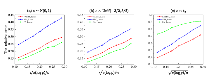
To illustrate the accuracy of our estimation, we set the number of latent factors to , the dimension of to , , the first entries of to 0.5, the remaining entries to 0. Throughout this subsection, we generate each entry of and from the standard Gaussian distribution , while each entry of is randomly generated from the uniform distribution . The is generated from the three scenarios: (a) the standard Gaussian distribution ; (b) the uniform distribution ; (c) . Under each setting, is set to satisfy that takes uniform grids in with step being 0.05.
To validate the necessities of considering latent factors in observational studies, we compare the relative error obtained by our approach (denoted as “FASIM_Lasso”) with the method in Rejchel and Bogdan, (2020) (denoted as “SIM_Lasso”), which considers the single-index model without incorporating the factor effect, and the method in Fan et al., (2024) (denoted as “FA_Lasso”). Figures 5 and 6 depict the relative error
of linear model (5.1) and nonlinear model (5.2), respectively. The simulation results indicate that for original data, FA_Lasso performs very well when the error is not heavy-tailed, but when the error follows the , FA_Lasso performs significantly worse. In contrast, the proposed method maintains stable and good performance across different error distribution scenarios, illustrating the robustness of our approach. Additionally, compared to SIM_Lasso, FASIM_Lasso enjoys smaller relative errors. This is partially due to the inadequacy of the SIM in Rejchel and Bogdan, (2020). Additionally, Figures 5 and 6 show that the upper limits of the statistical rates of FASIM_Lasso are , which validates Theorem 4.1.
To investigate the robustness of FASIM_Lasso, we introduce outliers into the observations using the aforementioned method, specifically, 10%+10(response). We output the of FA_Lasso and of FASIM_Lasso and SIM_Lasso. The results are depicted in Figures 7 and 8. The figures indicate that our proposed method can achieve more precise results, with smaller relative errors in all scenarios. This implies that our proposed method is much more robust than FA_Lasso confronted with outliers in the observed data.
5.3 Validity of confidence interval
In this subsection, we construct confidence intervals based on the proposed method in Section 4. We generate either from (a) or (b) and set , or . In addition, we generate , , and the parameters , as described in Section 5.2. To assess the performance of our methods, we examine the empirical coverage probabilities and the average lengths of confidence intervals for the individual coefficients across all covariates, covariates on and those on . We define
| CP | |||
The results are summarized in Table 2. The empirical coverage probabilities are close to the nominal level across all settings, and the average lengths of the confidence interval are very short. This illustrates the merits of our proposed methods. In addition, we find that even when the error follows a distribution, the average interval lengths only increase slightly.
Table 2 should be here.
6 Real data analysis
In this section, we employ our method with a macroeconomic dataset named FRED-MD (McCracken and Ng,, 2016) which comprises 126 monthly U.S. macroeconomic variables. Due to these variables measuring certain aspects of economic health, they are influenced by latent factors and thus can be regarded as intercorrelated. We analyze this dataset to illustrate the performance of FASIM and evaluate the adequacy of the factor regression model. In our study, we take “GS5” as response variable , and the remaining variables as predictors , where “GS5” represents the 5-year treasury rate. In addition, to demonstrate the robustness of FASIM, we apply the previously mentioned outlier handling method to the response variable, specifically using 10%+10(response). Due to the economic crisis of 2008-2009, the data remained unstable even after implementing the suggested transformations. Therefore, we examine data from two distinct periods: February 1992 to October 2007 and August 2010 to February 2020.
At the beginning, we employ our introduced FAST and FabTest in Fan et al., (2024) to test the adequacy of factor models, and denote the corresponding models with only factors as F_SIM and F_LM, respectively. We employ 2000 bootstrap replications here to obtain the critical value. For FabTest, we use 10 fold cross-validation to compute the tuning parameters and refit cross-validation based on iterated sure independent screening to estimate the variance of the error. The -values are provided in Table 3. At the significance level of 0.05, both for the original dataset and the polluted dataset, the results indicate the inadequacy of F_SIM for the “GS5” within the two distinct time periods. While for F_LM, the results indicate that it is inadequate for “GS5” in the original dataset within the two distinct time periods. When the data is polluted, the null hypothesis is rejected during the period from February 1992 to October 2007, while it is not rejected during the other period. This implies the necessary to introduce the idiosyncratic component into the regression model. Hence, in the subsequent study on prediction accuracy, we consider FASIM and FARM for comparison.
Table 3 should be here.
We compare the forecasting results of FASIM with that of FARM. For each given time period and model, predictions are performed using a moving window approach with a window size of 90 months. Indexing the panel data from 1 for each of the two time periods, for all , we use the 90 previous measurements to train the models (FASIM and FARM) and output predictions and . For FASIM, as defined in Equation (1), after obtaining the estimated parameters and , the estimated latent factor vector , and the estimated idiosyncratic component at the -th time point, we get the estimator of the unknown function via spline regression. Finally, the predicted value of the response variable is calculated as . The accuracy of FASIM and FARM is measured using the Mean Square Error (MSE) (Hastie et al.,, 2009), defined as:
where denotes the total number of data points in a given time period.
Table 4 should be here.
Table 4 presents the prediction accuracy results of FASIM and FARM of “GS5” for the original dataset and the polluted dataset within the two distinct time periods. It is evident that the performance of FASIM and FARM on the original data are similar. However, while the MSEs of both FASIM and FARM increase for the polluted dataset, the increase is substantial for FARM, whereas FASIM shows only a modest increase. This suggests that FASIM is more robust than FARM.
7 Conclusions and discussions
To capture nonliearity with latent factors, in this paper, we introduce a novel Factor Augmented sparse Single-Index Model, FASIM. For this newly proposed model, we first address the concern of whether the augmented part is necessary or not. We develop a score-type test statistic without estimating high-dimensional regression coefficients nor high-dimensional precision matrix. We also propose a Gaussian multiplier bootstrap to determine the critical value for our proposed test statistic FAST. The validity of our procedure is theoretically established under mild conditions. When the model test is passed, we employ the penalty to estimate the unknown parameters, establishing both and error bounds. We also introduce debiased estimator and establish its asymptotic normality. Numerical results illustrate the robustness and effectiveness of our proposed procedures.
In practice, it would be of interest to test whether the FASIM is actually FARM. We may also consider the multiple testing problem for the FASIM. Further the condition excludes even link functions, and in particular the problem of sparse phase retrieval. We would explore these possible topics in near future.
Appendix
Appendix A Proofs of Theorems
In the following, we will present the proofs of our main theorems. To save space, proofs of some technical lemmas will be shown in Supplementary Material.
A.1 Proof of Theorem 3.1
Proof.
By Lemma 2 in Supplementary Material, with high probability, we have
for some constant , as . Here . This implies that
| (A.1) |
For the term in (A.1), recall that with , by the sub-Gaussian assumptions of and , we can get that is a sub-Exponential variable sequence with bounded norm. In addition, by Assumption 3, applying Lemma 3 in Supplementary Material, we have
| (A.2) |
For the term in (A.1), by Lemma 4 in Supplementary Material, we have
| (A.3) |
Combining (A.2) with (A.1), we have
The proof is completed. ∎
A.2 Proof of Theorem 3.2
Proof.
A.3 Proof of Theorem 3.3
Proof.
Firstly, we have the following decomposition
| (A.6) |
For the term in (A.6), denoted , we have , with by Lemma 2 in Supplementary Material. For simplify, we rewrite , where . Under Assumption 1, it’s easy to show that is an i.i.d. mean zero sub-Exponential random variable sequence. Assume that . Denote , by the Bernstein’s inequality, we have
| (A.7) |
with probability at least . Therefore, with high probability, we have
| (A.8) |
For any , we have
| (A.9) |
Substituting (A.8) and (A.9) into (A.6), we have
By Theorem 3.2, is equal to the -th quantile of asymptotically. By (A.8), we have with high probability. Therefore,
The proof is completed. ∎
A.4 Proof of Theorem 4.1
Proof.
Recall that is the minimizer of optimization problem as
For the loss function in (4.2), to demonstrate the -norm error bound for , we aim to prove the following inequality:
| (A.10) |
where is the gradient of loss function , and , with positive constants and .
We firstly derive the upper bound of (A.10). By KKT condition, there exists a subgradient , such that . We then derive
| (A.11) |
Denote . For in (A.4), by the definition of subgradient, we have
| (A.12) |
where , and . For in (A.4), by Hlder’s inequality and Lemma 6 in Supplementary Material, we have
| (A.13) |
Recall that , and assume that . By triangle and Cauchy-Schwartz inequalities, combining (A.4) with (A.4), we have
| (A.14) |
The inequality (A.4) shows that the right side of (A.10) holds.
Next, we focus on proving the left side of (A.10). Note that for any ,
Because in (A.4), we have . Besides, we have the sparsity assumption that . Then, according to Lemma C.2 in Fan et al., (2024), we have
That is, with high probability, we have
| (A.15) |
which shows that the left side of (A.10) holds. Therefore, in conclusion, we prove the -norm error bound for , i.e.
| (A.16) |
where . Because in (A.4), we have
Therefore,
| (A.17) |
Here, .
The proof is completed.
∎
A.5 Proof of Theorem 4.2
Proof.
Recall that , with . Let be the i.i.d copies of . Namely, . We have the following decomposition.
Here, and . By Lemma 9 in Supplementary Material, as long as and , we have , where is given in Assumption 5. The proof is completed. ∎
References
- Ahn and Horenstein, (2013) Ahn, S. C. and Horenstein, A. R. (2013). Eigenvalue ratio test for the number of factors. Econometrica, 81(3):1203–1227.
- Bai, (2003) Bai, J. (2003). Inferential theory for factor models of large dimensions. Econometrica, 71(1):135–171.
- Bai and Ng, (2002) Bai, J. and Ng, S. (2002). Determining the number of factors in approximate factor models. Econometrica, 70(1):191–221.
- Bayle and Fan, (2022) Bayle, P. and Fan, J. (2022). Factor-augmented regularized model for hazard regression. arXiv preprint arXiv:2210.01067.
- Belloni et al., (2012) Belloni, A., Chen, D., Chernozhukov, V., and Hansen, C. (2012). Sparse models and methods for optimal instruments with an application to eminent domain. Econometrica, 80(6):2369–2429.
- Bing et al., (2023) Bing, X., Cheng, W., Feng, H., and Ning, Y. (2023). Inference in high-dimensional multivariate response regression with hidden variables. Journal of the American Statistical Association, pages 1–12.
- Bühlmann et al., (2014) Bühlmann, P., Kalisch, M., and Meier, L. (2014). High-dimensional statistics with a view toward applications in biology. Annual Review of Statistics and Its Application, 1(1):255–278.
- Cai et al., (2011) Cai, T., Liu, W., and Luo, X. (2011). A constrained minimization approach to sparse precision matrix estimation. Journal of the American Statistical Association, 106(494):594–607.
- Cai et al., (2014) Cai, T., Liu, W., and Xia, Y. (2014). Two-sample test of high dimensional means under dependence. Journal of the Royal Statistical Society Series B: Statistical Methodology, 76(2):349–372.
- Cai et al., (2016) Cai, T., Liu, W., and Zhou, H. H. (2016). Estimating sparse precision matrix: Optimal rates of convergence and adaptive estimation. Annals of Statistics, 44(2):455–488.
- Ćevid et al., (2020) Ćevid, D., Bühlmann, P., and Meinshausen, N. (2020). Spectral deconfounding via perturbed sparse linear models. Journal of Machine Learning Research, 21(1):9442–9482.
- Chernozhukov et al., (2023) Chernozhukov, V., Chetverikov, D., and Koike, Y. (2023). Nearly optimal central limit theorem and bootstrap approximations in high dimensions. Annals of Applied Probability, 33(3):2374–2425.
- Cook and Ni, (2005) Cook, R. D. and Ni, L. (2005). Sufficient dimension reduction via inverse regression: A minimum discrepancy approach. Journal of the American Statistical Association, 100(470):410–428.
- Dezeure et al., (2017) Dezeure, R., Bühlmann, P., and Zhang, C. (2017). High-dimensional simultaneous inference with the bootstrap. Test, 26(4):685–719.
- Eftekhari et al., (2021) Eftekhari, H., Banerjee, M., and Ritov, Y. (2021). Inference in high-dimensional single-index models under symmetric designs. Journal of Machine Learning Research, 22(27):1–63.
- Fan et al., (2022) Fan, J., Guo, J., and Zheng, S. (2022). Estimating number of factors by adjusted eigenvalues thresholding. Journal of the American Statistical Association, 117(538):852–861.
- Fan et al., (2020) Fan, J., Li, R., Zhang, C., and Zou, H. (2020). Statistical foundations of data science. Chapman and Hall/CRC.
- Fan et al., (2013) Fan, J., Liao, Y., and Mincheva, M. (2013). Large covariance estimation by thresholding principal orthogonal complements. Journal of the Royal Statistical Society Series B: Statistical Methodology, 75(4):603–680.
- Fan et al., (2018) Fan, J., Liu, H., and Wang, W. (2018). Large covariance estimation through elliptical factor models. Annals of Statistics, 46(4):1383.
- Fan et al., (2024) Fan, J., Lou, Z., and Yu, M. (2024). Are latent factor regression and sparse regression adequate? Journal of the American Statistical Association, 119(546):1076–1088.
- Fan et al., (2019) Fan, J., Wang, W., and Zhong, Y. (2019). Robust covariance estimation for approximate factor models. Journal of Econometrics, 208(1):5–22.
- Fan et al., (2017) Fan, J., Xue, L., and Yao, J. (2017). Sufficient forecasting using factor models. Journal of Econometrics, 201(2):292–306.
- Fewell et al., (2007) Fewell, Z., Davey Smith, G., and Sterne, J. A. (2007). The impact of residual and unmeasured confounding in epidemiologic studies: a simulation study. American Journal of Epidemiology, 166(6):646–655.
- Guo et al., (2022) Guo, Z., Ćevid, D., and Bühlmann, P. (2022). Doubly debiased lasso: High-dimensional inference under hidden confounding. Annals of Statistics, 50(3):1320.
- Hall and Li, (1993) Hall, P. and Li, K.-C. (1993). On almost linearity of low dimensional projections from high dimensional data. Annals of Statistics, 21(2):867–889.
- Han et al., (2023) Han, D., Han, M., Huang, J., and Lin, Y. (2023). Robust inference for high-dimensional single index models. Scandinavian Journal of Statistics, 50(4):1590–1615.
- Hastie et al., (2009) Hastie, T., Tibshirani, R., Friedman, J. H., and Friedman, J. H. (2009). The elements of statistical learning: data mining, inference, and prediction, volume 2. Springer.
- Jiang et al., (2019) Jiang, F., Ma, Y., and Wei, Y. (2019). Sufficient direction factor model and its application to gene expression quantitative trait loci discovery. Biometrika, 106(2):417–432.
- Kim and Mueller, (1978) Kim, J.-O. and Mueller, C. W. (1978). Factor analysis: Statistical methods and practical issues, volume 14. sage.
- Kong and Xia, (2007) Kong, E. and Xia, Y. (2007). Variable selection for the single-index model. Biometrika, 94(1):217–229.
- Lam and Yao, (2012) Lam, C. and Yao, Q. (2012). Factor modeling for high-dimensional time series: inference for the number of factors. Annals of Statistics, 40(2):694–726.
- Li, (1991) Li, K.-C. (1991). Sliced inverse regression for dimension reduction. Journal of the American Statistical Association, 86(414):316–327.
- Li and Duan, (1989) Li, K.-C. and Duan, N. (1989). Regression analysis under link violation. Annals of Statistics, 17(3):1009–1052.
- Listgarten et al., (2010) Listgarten, J., Kadie, C., Schadt, E. E., and Heckerman, D. (2010). Correction for hidden confounders in the genetic analysis of gene expression. Proceedings of the National Academy of Sciences, 107(38):16465–16470.
- Luo et al., (2009) Luo, R., Wang, H., and Tsai, C.-L. (2009). Contour projected dimension reduction. Annals of Statistics, 37:3743–3778.
- Luo et al., (2022) Luo, W., Xue, L., Yao, J., and Yu, X. (2022). Inverse moment methods for sufficient forecasting using high-dimensional predictors. Biometrika, 109(2):473–487.
- Ma et al., (2021) Ma, R., Cai, T., and Li, H. (2021). Global and simultaneous hypothesis testing for high-dimensional logistic regression models. Journal of the American Statistical Association, 116(534):984–998.
- McCracken and Ng, (2016) McCracken, M. W. and Ng, S. (2016). Fred-md: A monthly database for macroeconomic research. Journal of Business and Economic Statistics, 34(4):574–589.
- Ning and Liu, (2017) Ning, Y. and Liu, H. (2017). A general theory of hypothesis tests and confidence regions for sparse high dimensional models. Annals of Statistics, 45(1):158–195.
- Ouyang et al., (2023) Ouyang, J., Tan, K. M., and Xu, G. (2023). High-dimensional inference for generalized linear models with hidden confounding. Journal of Machine Learning Research, 24(296):1–61.
- Plan and Vershynin, (2016) Plan, Y. and Vershynin, R. (2016). The generalized lasso with non-linear observations. IEEE Transactions on Information Theory, 62(3):1528–1537.
- Radchenko, (2015) Radchenko, P. (2015). High dimensional single index models. Journal of Multivariate Analysis, 139:266–282.
- Rejchel and Bogdan, (2020) Rejchel, W. and Bogdan, M. (2020). Rank-based lasso-efficient methods for high-dimensional robust model selection. Journal of Machine Learning Research, 21(244):1–47.
- Sun et al., (2023) Sun, Y., Ma, L., and Xia, Y. (2023). A decorrelating and debiasing approach to simultaneous inference for high-dimensional confounded models. Journal of the American Statistical Association, (to appear):1–24.
- Tibshirani, (1996) Tibshirani, R. (1996). Regression shrinkage and selection via the lasso. Journal of the Royal Statistical Society Series B: Statistical Methodology, 58(1):267–288.
- Van de Geer et al., (2014) Van de Geer, S., Bühlmann, P., Ritov, Y., and Dezeure, R. (2014). On asymptotically optimal confidence regions and tests for high-dimensional models. Annals of Statistics, 42(3):1166–1202.
- Verzelen, (2012) Verzelen, N. (2012). Minimax risks for sparse regressions: Ultra-high dimensional phenomenons. Electronic Journal of Statistics, 6:38–90.
- Wang et al., (2012) Wang, T., Xu, P., and Zhu, L. (2012). Non-convex penalized estimation in high-dimensional models with single-index structure. Journal of Multivariate Analysis, 109:221–235.
- Yang et al., (2024) Yang, W., Shi, H., Guo, X., and Zou, C. (2024). Robust group and simultaneous inferences for high-dimensional single index model. Manuscript.
- Zhang and Zhang, (2014) Zhang, C. and Zhang, S. S. (2014). Confidence intervals for low dimensional parameters in high dimensional linear models. Journal of the Royal Statistical Society Series B: Statistical Methodology, 76(1):217–242.
- Zhang and Cheng, (2017) Zhang, X. and Cheng, G. (2017). Simultaneous inference for high-dimensional linear models. Journal of the American Statistical Association, 112(518):757–768.
- Zhu and Zhu, (2009) Zhu, L. and Zhu, L. (2009). Nonconcave penalized inverse regression in single-index models with high dimensional predictors. Journal of Multivariate Analysis, 100(5):862–875.
Figures


Tables
| FAST_i | FabTest_i | FAST_ii | FabTest_ii | ||
|---|---|---|---|---|---|
| 1.50 | 46.33 | 1.60 | 44.53 | ||
| 1.61 | 45.62 | 1.48 | 47.08 | ||
| 3.72 | 156.00 | 3.75 | 156.53 | ||
| 3.65 | 208.86 | 3.73 | 146.21 |
| Model | CP | AL | ||||||
|---|---|---|---|---|---|---|---|---|
| Model 1 | 500 | 0.951 | 0.955 | 0.951 | 0.040 | 0.039 | 0.040 | |
| 0.947 | 0.950 | 0.947 | 0.066 | 0.064 | 0.066 | |||
| 200 | 0.952 | 0.940 | 0.952 | 0.040 | 0.039 | 0.040 | ||
| 0.946 | 0.943 | 0.946 | 0.067 | 0.066 | 0.067 | |||
| Model 2 | 500 | 0.951 | 0.966 | 0.951 | 0.041 | 0.040 | 0.041 | |
| 0.946 | 0.930 | 0.946 | 0.069 | 0.068 | 0.069 | |||
| 200 | 0.951 | 0.974 | 0.950 | 0.041 | 0.040 | 0.041 | ||
| 0.947 | 0.956 | 0.947 | 0.067 | 0.066 | 0.067 |
| Time Period | Data | F_SIM | F_LM |
|---|---|---|---|
| 1992.02-2007.10 | original | 0.0000 | |
| polluted | 0.0000 | 0.0000 | |
| 2010.08-2020.02 | original | 0.0000 | |
| polluted | 0.0000 | 0.2015 |
| Time Period | Data | FARM | FASIM |
|---|---|---|---|
| 1992.02-2007.10 | original | 0.2620 | 0.2764 |
| polluted | 1.0592 | 0.9251 | |
| 2010.08-2020.02 | original | 0.3328 | 0.3748 |
| polluted | 0.9432 | 0.8764 |