High-Dimensional Data Set Simplification by Laplace-Beltrami Operator

Let $M$ be a Riemannian manifold (differentiable manifold with Riemannian metric), and $f\in C^{2}$ be a real-valued function defined on $M$. The LBO $\Delta$ on $M$ is defined as

where $grad\ f$ is the gradient of $f$, and $div(\cdot)$ is the divergence on $M$. The LBO (1) can be represented in local coordinates. Let $\psi$ be a local parametrization

of a sub-manifold of $M$ with

where $i,j=1,2,...,n$ , $\langle,\rangle$ is the dot product, and $det$ is the determinant. In the local coordinates, the LBO (1) can be transformed as,

The eigenvalues and eigenfunctions of the LBO (1) (2) can be calculated by solving the Helmholtz equation:

where $\lambda$ is a real number. The spectrum of LBO is a list of eigenvalues such as

with the corresponding eigenfunctions,

which are orthogonal.

In the case of a closed manifold, the first eigenvalue $\lambda_{0}$ is always zero. Moreover, the eigenvalues $\lambda_{i},i=0,1,2,\cdots$ (4) specify the discrete frequency domain of an LBO, and the eigenfunctions are the extensions of the basis functions in Fourier analysis to a manifold. Eigenfunctions of larger eigenvalues contain higher frequency information. It is well known that the eigenvalues and eigenfunctions of an LBO are closely related to the geometric properties of the manifold where the LBO is defined, including its curvature [37], volume of $M$, volume of $\partial{M}$, and Euler characteristic of $M$ [11].

Specifically, consider a heat diffusion equation defined on a closed manifold $M$ (i.e., $\partial M={\O}$):

where $x\in M$, $u(x,t)$ is the heat value of the point $x$ at time $t$, and $f$ is the initial heat distribution on $M$. The solution of the heat diffusion equation (6) can be expressed as:

where, $H(x,y,t)$ is the fundamental solution of the heat diffusion equation (6), called heat kernel. The heat kernel $H(x,y,t)$ measures the amount of heat transferred from $x$ to $y$ within time $t$, and can be rewritten as,

where $\lambda_{i},i=0,1,\cdots$ (4) are the eigenvalues of the LBO (1) (2), and $\phi_{i},i=0,1,\cdots$ (5) are the corresponding eigenfunctions.

When $x=y$ in Eq. (7), $H(x,x,t)$ , called HKS, quantifies the change of heat at $x$ along the time $t$. It has been shown that [38, 39, 37], when the time $t$ approaches $0^{+}$ sufficiently close, the heat kernel $H(x,x,t)$ can be represented as,

where $K(x)$ is the scalar curvature at point $x$ on $M$. Especially, when $M$ is a 2-dimensional manifold, $K(x)$ is the Gaussian curvature at $x$.

From Eq. (8), we can see that, the eigenfunctions $\phi_{i}(x),i=0,1,\cdots$ (5) of a LBO are closely related to the scale curvature $K(x)$ at the point $x\in M$.

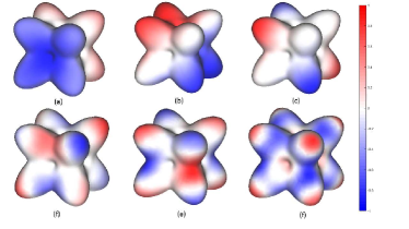
As stated above, the eigenfunctions $\phi_{i}(x),i=0,1,\cdots$ (5) are the extension of the trigonometric functions. In the trigonometric function system, the local extrema of a trigonometric function with a lower frequency hold in the trigonometric function with a higher frequency (Fig. 1). This property is preserved by the eigenfunctions $\phi_{i}(x),i=0,1,\cdots$ (5) on manifolds. In Fig. 2, eigenfunctions of an LBO defined on a 2D manifold are illustrated with their local extrema. We can observe that, the local extrema in the lower frequency eigenfunctions remain the local extrema in the higher frequency eigenfunctions (Fig. 2). Because the local extrema of $\phi_{i}(x)$ hold in $\phi_{j}(x),j<i$, and the heat kernel (8) is a weighted sum of $\phi_{i}^{2}(x),i=0,1,\cdots$, the local extrema of $\phi_{i}(x)$, especially the eigenfunctions with low frequency, are the candidates of the local extrema of the heat kernel $H(x,x,t)$ (8), and the scale curvature $K(x)$ (8). In conclusion, the local extrema of the eigenfunctions $\phi_{i}(x),i=0,1,\cdots$ contain the features of the manifold where the LBO is defined. Therefore, in this paper, we use the local extrema of the eigenfunctions of the LBO defined on a high-dimensional data set as its feature points, which constitute the simplified data set.

To solve the Helmholtz equation (3) for calculating the eigenvalues and eigenfunctions of the LBO (2), the Helmholtz equation (3) must be discretized into a linear system of equations. Traditionally, Eq. (3) is discretized on a mesh with connectivity information between two mesh vertices [4, 14, 2]. However, in this paper, we are addressing an unorganized data point set in a high-dimensional space, where the connectivity information is missing. Hence, we use the discretization method developed in [14] to construct the discrete LBO. Because only the Euclidean distances between points are involved in the construction of the discrete LBO, it can be employed for LBO discretization in high-dimensional space.

The LBO discretization method [14] contains the two steps:

• •

  adjacency graph construction,

• •

  weight computation,

which are explained in detail in the following.

Adjacency graph construction. There are two methods for constructing an adjacency graph: (a) $k$ nearest neighbors (KNN). For any vertex $v$, its $k$ nearest neighbors $v_{i},i=1,2,\cdots,k$ are determined using the KNN algorithm [40]. Then, the connection between the vertex $v$ and each neighbor $v_{i},i=1,2,\cdots,k$ is established, thus constructing the adjacent graph. Because the $k$ nearest neighbors are not symmetric, i.e., it is possible that the vertex $v_{i}$ is in the $k$ nearest neighbors of the vertex $v_{j}$, yet, $v_{j}$ is not in the $k$ nearest neighbors of $v_{i}$, the weight matrix (see below) constructed by the KNN method is not guaranteed to be symmetric. (b) $\epsilon$ -neighbors. For a vertex $v$, a hypersphere is first constructed, which uses $v$ as the center, and $\epsilon$ as its radius. The adjacency graph is constructed by connecting the vertex $v$ and each vertex lying in the hypersphere. Although the weight matrix constructed based on the $\epsilon$ -neighbors is symmetric, there is a serious problem in that the value of $\epsilon$ is difficult to choose. An overly small $\epsilon$ will cause certain rows of the weight matrix $W$ to be zero; and overly large $\epsilon$ will create a matrix that is excessively dense. Therefore, in our implementation, we employ the $k$ nearest neighbors to construct the adjacency matrix.

Weight computation. Using the adjacency graph for each point $v_{i}$ in the given data set, the connections between point $v_{i}$ and the other points in the data set are established. Based on the adjacency graph, the weights between point $v_{i}$ and each of the other points can be calculated as follows:

Because only the Euclidean distance $\left\|v_{i}-v_{j}\right\|$ is required in the computation of $w_{ij}$, it is appropriate for addressing high-dimensional data sets.

As stated above, the weight matrix $\bar{W}=[w_{ij}]$ (9) constructed by the KNN method is not symmetric, so we take the following matrix:

as the weight matrix, which is a symmetric matrix. Moreover, we construct a diagonal matrix

where $a_{i}=w_{ii}$ (refer to Eq. (9)). Then the LBO can be discretized into the matrix,

whatever the dimension of the space the LBO defined on. Meanwhile, the Helmholtz equation (3) is discretized as,

where $\lambda$ is the eigenvalue of the Laplace matrix $L$, and $\varphi$ is the corresponding eigenvector. It is equivalent to,

Because the matrix $W$ is symmetric, and the matrix $A$ is diagonal, it has been shown that the eigenvalues $\lambda$ are all non-negative real numbers satisfying  [3]:

and the corresponding eigenvectors $\varphi_{i},i=1,2,\cdots,n$ are orthogonal, i.e.,

By solving Eq. (10), the eigenvalues $\lambda_{1}\leq\lambda_{2}\leq\cdots\leq\lambda_{n}$ and the corresponding eigenvectors $\varphi_{i},i=1,2,\cdots,n$ are determined. The local maximum, minimum, and saddle points of the eigenvectors are used as the feature points. As stated above, the eigenvalue $\lambda_{i}$ measures the ’frequency’ of its corresponding eigenvector $\varphi_{i}$. The larger the eigenvalue, the higher the frequency of the eigenvector $\varphi_{i}$, and then the greater number of feature points in the eigenvector $\varphi_{i}$. The data simplification algorithm first detects the feature points of the eigenvector $\varphi_{1}$, and adds them to the simplified data set. Then, it detects and adds the feature points of $\varphi_{2}$ to the simplified data set. This procedure is performed iteratively until the simplified data set satisfies a preset fidelity threshold to the original data point set, according to the metrics defined in Section 3.4.

Because each of the eigenvectors $\varphi_{i},i=1,2,\cdots,n$ is a scalar function defined on an unorganized point set in a high-dimensional space, the detection of the maximum, minimum, and saddle points on the defined function is not straightforward. Suppose $\omega(x)$ is a scalar function defined on each point of an unorganized data point set. For each point $x$ in the data set, we construct its neighbor $N_{x}$ using the KNN algorithm, discussed previously in Section3.2. The methods for detecting the maximum, minimum, and saddle points of the function $\omega(x)$ are elucidated in the following.

Maximum and minimum point detection: For a data point $x$ in the data set and any data point $y\in N_{x}$, if $\omega(y)<\omega(x)$, $\forall y\in N_{x}$, the data point $x$ is a local maximum point of $\omega(x)$. Conversely, if $\omega(y)>\omega(x)$, $\forall y\in N_{x}$, the data point $x$ is a local minimum point of $\omega(x)$.

Saddle point detection: To detect the saddle points of $\omega(x)$ defined on an unorganized high-dimensional data point set, the points of the set are projected into a 2D plane, using the DR methods [14]. The data point projected into a 2D plane continues to be denoted as $x$. For a point $x$, the points in its KNN neighbor $N_{x}$ comprise its one-ring neighbor $R_{x}$ (see Fig. 3). Each point $x_{r}$ in $R_{x}$ has a sole preceding point $x_{r}^{p}$ and a sole succeeding point $x_{r}^{n}$ in a counter-clockwise direction. As illustrated in Fig. 3, if $\omega(x)\geq\omega(x_{r})$, the point $x_{r}$ is labeled as $\ominus$; otherwise, it is labeled as $\oplus$. Now, we initialize a counter $sum=0$ and traverse the one-ring neighbor $R_{x}$ of point $x$ from an arbitrary point. If the signs of two neighbor points in $R_{x}$ are different (marked with dotted lines), $sum=sum+1$. Finally, if the counter $sum\geq 4$, point $x$ is a saddle point; otherwise, it is not a saddle point (Fig. 3). Examples of saddle points and non-saddle points are demonstrated in Fig. 3.

As stated in Section 3.3, the data simplification method detects the feature points of the eigenvectors $\varphi_{i},i=1,2,\cdots,n$, and adds them to the simplified data set iteratively, until the simplified data set satisfies a preset threshold of fidelity to the original data set. In this section, three metrics are devised to measure the fidelity of the simplified data set $\mathcal{S}$ to the original high-dimensional data set $\mathcal{H}$; these are the Kullback-Leibler divergence (KL divergence) [41]-based metric, Hausdorff distance [42], and determinant of covariance matrix [43]. They measure the fidelity of the simplified data set $\mathcal{S}$ to the original data set $\mathcal{H}$ from three aspects:

• •

  entropy of information (KL-divergence-based metric),

• •

  distance between two sets (Hausdorff distance),and

• •

  ’volume’ of a data set (determinant of covariance matrix).

KL-divergence-based metric. KL-divergence [41], also called relative entropy, is typically employed to measure the difference between two probability distributions $P=\{p_{i}\}$ and $Q=\{q_{i}\}$, i.e.,

To define the KL-divergence-based metric, the original data set $\mathcal{H}$ and simplified data set $\mathcal{S}$ are represented as an $n\times d$ matrix $M_{\mathcal{H}}$, and an $m\times d$ matrix $M_{\mathcal{S}}$, where $n,m,(n>m)$ are the number of data points in the data sets $\mathcal{H}$ and $\mathcal{S}$, respectively. Each row of the matrices $\mathcal{H}$ and $\mathcal{S}$ stores a data point in the $d-$dimensional Euclidean space. First, we calculate the probability distribution $P^{(k)}=\{p^{(k)}_{i}\},k=1,2,\cdots,d$ for each dimension of the data points in the original data set $\mathcal{H}$, corresponding to the $k^{th}$ column of matrix $M_{\mathcal{H}}$. To do this, the $k^{th}$ column elements of matrix $M_{\mathcal{H}}$ are normalized into the interval $[0,1]$, which is divided into $l$ subintervals, (in our implementation, we use $l=100$). By counting the number of elements of the $k^{th}$ column of matrix $M_{\mathcal{H}}$ whose values lie in the $l$ subintervals, the value distribution histogram is generated, which is then used as the probability distribution $P^{(k)}=\{p^{(k)}_{i},i=1,2,\cdots,l\}$ of the $k^{th},k=1,2,\cdots,d$ column of matrix $M_{\mathcal{H}}$. Similarly, the probability distribution $Q^{(k)}=\{q^{(k)}_{i},i=1,2,\cdots,l\}$ of the $k^{th},k=1,2,\cdots,d$ column of matrix $M_{\mathcal{S}}$ can be calculated. Then, the KL-divergence for the $k^{th},k=1,2,\cdots,d$ column elements of matrix $M_{\mathcal{H}}$ and $M_{\mathcal{S}}$ is

And the KL-divergence-based metric is defined as

The KL-divergence-based metric (12) transforms the high-dimensional data set into its probability distribution, and measures the difference between the probability distributions of the original and simplified data sets. As the simplified data set $\mathcal{S}$ becomes increasingly closer to the original data set $\mathcal{H}$, the KL-divergence-based metric $d_{KL}$ becomes increasingly smaller. When $\mathcal{S}=\mathcal{H}$, $d_{KL}=0$.

Hausdorff distance. The Hausdorff distance [42] measures how far two sets are away from each other. Suppose $\mathcal{X}$ and $\mathcal{Y}$ are two data set in $d-$dimensional space, and denote

the maximum distance from an arbitrary point in set $\mathcal{X}$ to set $\mathcal{Y}$, where $d(x,y)$ is the Euclidean distance between two points $x$ and $y$. The Hausdorff distance between the original data set $\mathcal{H}$ and simplified data set $\mathcal{S}$ is defined as

Note that the simplified data set $\mathcal{S}$ is a subset of the original data set $\mathcal{H}$, and then, $D(\mathcal{S},\mathcal{H})=0$. Therefore, the Hausdorff distance between $\mathcal{H}$ and $\mathcal{S}$ can be calculated by

That is, the Hausdorff distance is the maximum distance from an arbitrary point in the original data set $\mathcal{H}$ to the simplified data set $\mathcal{S}$.

Determinant of covariance matrix. The covariance matrix is frequently employed in statistics and probability theory to measure the joint variability of several variables [43]. Suppose

are $m$ samples in a $d-$dimensional sample space $X$, and denote

where $\bar{X}_{j}$ is the mean value of the $j$-th random variable. The covariance $c_{ij}$ between the $i$-th and $j$-th random variables is

which is the $(i,j)^{th}-$element of the covariance matrix $Cov(X)$ of the data set $X$. According to  [43], the determinant of the covariance matrix of $X$, i.e., $det(Cov(X))$, can express the ’volume’ of the data set $X$. When the simplified data set $\mathcal{S}$ approaches the original data set $\mathcal{H}$, they are expected to have increasingly ’volumes’, namely, the determinants of covariance matrices. Therefore, the difference of the determinants of the covariance matrices of $\mathcal{H}$ and $\mathcal{S}$:

can measure the fidelity of the simplified data set $\mathcal{S}$ to the original data set $\mathcal{H}$.

In this section, we will illustrate several data simplification results.

Swiss roll: In Fig. 5, we use the swiss roll data set in 3D space to illustrate the intuitive simplification procedure by the proposed data simplification algorithm. In Fig 5, the simplified data set is generated by detecting the feature points of the first five eigenvectors, which captures the critical points at the head and tail positions of the roll (marked in red and blue colors). In Figs. 5- 5, by detecting higher frequency eigenvectors, increasingly more feature points are added into the simplified data set and it approaches increasingly closer to the original data set (Fig. 5). Note that the simplified data set in Fig. 5, which contains $397$ data points (approximately $20\%$ points of the entire data set), includes the majority of the information of the original data set. Please refer to Section 4.2 for the quantitative fidelity analysis of the simplified data set to the original data set measured by the metrics $d_{KL}$ (12), $d_{H}$ (13), and $d_{COV}$ (14).

MNIST: For clarity of the visual analysis, we selected $900$ units of the gray images for the digits ’0’ to ’4’, from the MNIST data set, and resized each image as $8\times 8$. The selected handwritten digit images were projected into the 2D-plane using the DR method T-SNE [48]. Whereas in Fig. 6, colorful digits are placed at the projected 2D points, in Fig. 6, the images themselves are located at the projected points. The simplified data sets with $82,120,196,280$ data points, which were generated by detecting the feature points of the first $5,10,20,30$ LBO eigenvectors are displayed in Fig. 6- 6. For illustration, their positions in the 2D-plane are extracted from the dimensionality reduced data set (Fig. 6). In the simplified data set in Fig. 6, which has $82$ data points (approximately $9\%$ of the points of the original data set), all five categories of the digits are represented. In the simplified data set in Fig. 6, which has $196$ data points (approximately $22\%$ of the points of the original data set), virtually all of the key features of the data set are represented, including the subset of digit ’2’ in the class of digit ’1’. In Fig. 6, the simplified data set contains $280$ data points (approximately $31\%$ of the points of the original data set). We can observe that the boundary of each class of data points has formed (Fig. 6), and the geometric shape of each class is similar to that of the corresponding class in the original data set (Fig. 6).

Human face: The human face data set (Fig. 4) contains $698$ gray-images($64\times 64$) of a plaster head sculpture. The images of the data set were captured by adjusting three parameters: up-down pose, left-right pose, and lighting direction. Therefore, the images in the data set can be regarded as distributing on a 3D-manifold. Thus, as illustrated in Fig. 7, after the human face data set is dimensionally reduced into a 2D-plane using PCA [49], it can observed that the longitudinal axis represents the sculpture’s rotation in the right-left direction, and the horizontal axis indicates the change of lighting.

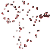
In Fig. 7, the images marked with red frames constitute the simplified data set. The simplified data sets in Figs. 7- 7 which consist of $16,40,95,150,270$ data points, are generated by detecting the feature points of the first $5,10,20,30,50$ LBO eigenvectors, respectively. In the simplified data set in Fig. 7, the critical points at the boundary are captured. In Figs. 7- 7, increasingly more critical points at the boundary and interior are added into the simplified data sets. In Fig. 7, virtually all of the images at the boundary are added into the simplified set. For clarity, we display the feature points of the first five LBO eigenvectors in Fig. 7, which indeed capture several ’extreme’ images in the human face data set. Specifically, the two feature points of the first eigenvector, $\phi_{1}$, are two images with ’leftmost pose + most lighting’ and ’rightmost pose + most lighting’. In the feature point set of the second eigenvector, $\phi_{2}$, an image with ’leftmost pose + fewest lighting’ is added. Similarly, in the feature point sets of the eigenvectors $\phi_{3},\phi_{4}$, and $\phi_{5}$, there are ’extreme’ images of the pose and lighting (Fig. 7).

CIFAR-10: The data set CIFAR-10 (Fig. 4) was also simplified by the proposed method. Similarly, increasingly more critical points of the data set were added into the simplified data set as a consequence of the simplification procedure.

The fidelity of the simplified data sets was quantitatively measured as per Section 4.2. In Table I, The running time in seconds of the proposed method is listed. It can be seen that the operations of KNN and eigen-solving consume the majority of the time, and the data simplification time ranged from $0.044$ to $4.759$ seconds.

In this section, the fidelity of the simplified data set $\mathcal{S}$ to the original data set $\mathcal{H}$ is quantitatively measured by the three metrics developed in Section 3.4, i.e., KL-divergence-based metric $d_{KL}(\mathcal{H},\mathcal{S})$ (12), Hausdorff distance $d_{H}(\mathcal{H},\mathcal{S})$ (13), and determinant of covariance matrix $d_{COV}(\mathcal{H},\mathcal{S})$ (14). Specifically, for the data simplification procedure of each of the four data sets mentioned above, a series of simplified data sets $\mathcal{S}_{i},i=1,2,\cdots,n$ was first generated. Then, we calculated the simplification rate $r_{i}$, i.e., the ratio between the cardinality of each data set $\mathcal{S}_{i}$ and that of the original data set $\mathcal{H}$, i.e.,

and the three metrics

which were normalized into $[0,1]$. Finally, the diagrams of $r_{i}$ v.s. $d_{KL}(\mathcal{H},\mathcal{S}_{i})$, $r_{i}$ v.s. $d_{H}(\mathcal{H},\mathcal{S}_{i})$, and $r_{i}$ v.s. $d_{COV}(\mathcal{H},\mathcal{S}_{i}),i=1,2,\cdots,n$ were plotted as displayed in Figs. 8, 9, and 10, respectively.

KL-divergence-based metric: $d_{KL}(\mathcal{H},\mathcal{S})$ (12) measures the similarity of the distributions of the simplified data set $\mathcal{S}$ and the original data set $\mathcal{H}$. If $\mathcal{S}$ is exactly the same as $\mathcal{H}$, then $d_{KL}(\mathcal{H},\mathcal{S})=0$.

Fig. 8 displays the diagrams of $r_{i}=\frac{Card(\mathcal{S}_{i})}{Card(\mathcal{H})}$ v.s. the normalized $d_{KL}(\mathcal{H},\mathcal{S}_{i}),i=1,2,\cdots,n$ of the four data sets. It can be observed that in the simplification procedures of all of four data sets, the metric $d_{KL}(\mathcal{H},\mathcal{S})$ is rapidly reduced to a small value (less than 0.1), when $r_{i}=0.1$ , approximately, i.e., the simplified data set contains approximately $10\%$ of the data points of the original data set. Using the data set swiss roll as an example (blue line) when the simplified data set $\mathcal{S}$ is composed of $5\%$ of the data points of the original data set $\mathcal{H}$ (i.e., $r_{i}=0.05$), the normalized $d_{KL}(\mathcal{H},\mathcal{S})$ is less than $0.1$; when $r_{i}=0.2$ ($\mathcal{S}$ contains $20\%$ of the data points of $\mathcal{H}$), the normalized $d_{KL}(\mathcal{H},\mathcal{S})$ is close to $0$, meaning that the simplified data set $\mathcal{S}$ contains virtually all of the information embraced by the original data set $\mathcal{H}$.

The Hausdorff distance $d_{H}(\mathcal{H},\mathcal{S})$ (13) measures the geometric distance between two sets. In Fig. 9, the diagram between

is illustrated. Because the Hausdorff distances between the original data set $\mathcal{H}$ and two adjacent simplified data sets, e.g., $d_{H}(\mathcal{H},\mathcal{S}_{i})$ and $d_{H}(\mathcal{H},\mathcal{S}_{i+1}),i=1,2,\cdots,n-1$, are possibly the same, the diagrams demonstrated in Fig. 9 are step-shaped. Based on Fig. 9, in the data simplification procedures of the four data sets, the Hausdorff distances $d_{H}(\mathcal{H},\mathcal{S})$ decrease when increasingly more data points are contained in the simplified data sets. Moreover, the convergence speed of $d_{H}(\mathcal{H},\mathcal{S}_{i})$ with respect to $r_{i}$ (15) is related to the intrinsic dimension of the data set: The lower the intrinsic dimension of a data set, the faster the convergence speed. For example (refer to Fig. 9), the intrinsic dimension of the data set swiss roll is $2$ (the smallest of the four data sets), and the convergence speed of the diagram for the simplification procedure of swiss roll is the fastest. The intrinsic dimension of the data set human face is $3$, greater than that of swiss roll, and the convergence speed of its diagram is slower than that of swiss roll. The intrinsic dimensions of the data sets MNIST and CIFAR-10 are greater than those of swiss roll and human face, and the convergence speeds of their diagrams are the slowest.

The determinant of covariance matrix of a data set reflects its ’volume’. The metric $d_{COV}(\mathcal{H},\mathcal{S})$ (14) measures the difference between the ’volume’ of the original data set $\mathcal{H}$ and that of the simplified data set $\mathcal{S}$. In Fig. 10, the diagram of $r_{i}$ (15) v.s. the normalized $d_{COV}(\mathcal{H},\mathcal{S}_{i}),i=1,2,\cdots,n$ is illustrated. In the region with small $r_{i}$ (15), the simplified data set contains a small number of data points and the diagrams oscillate. This is because the ’volume’ of a simplified data set with a small number of data points is heavily influenced by each of its points, and adding merely one point into the set can change its ’volume’ significantly. However, with increasingly more data points inserted into the simplified data set (i.e., with increasingly greater $r_{i}$), the diagrams of all four data sets converge to zero. Considering the data set CIFAR-10 as an example, when the simplified data set contains $20\%$ of the data points of the original data set ($r_{i}=0.2$), the metric $d_{COV}(\mathcal{H},\mathcal{S})$ (14) is nearly zero, meaning that the ’volume’ of the simplified data set has approached that of the original data very closely.

In this section, two applications of the proposed data set simplification method are demonstrated; there are the speedup of DR and training data simplification in supervised learning.

Speedup of DR: The computation of the DR algorithms for a high-dimensional data set is typically complicated. Given an original data set $\mathcal{H}$ ($Card(\mathcal{H})=n$), if we first perform the DR on the simplified data set $\mathcal{S}$ ($Card(\mathcal{S})=m$), and then employ the ’out-of-sample’ algorithm [50] to calculate the DR coordinates of the remaining data points, the computation requirement can be reduced significantly. Because the simplified data set $\mathcal{S}$ captures the feature points of the original data set, the result generated by DR on simplified set + ’out-of-sample’ is similar as that by DR on original set.

First, we compare the results of DR on the simplified data sets and that of DR on the original data set. Here, the data set human face is used as the original set and its simplified data sets are $\mathcal{S}_{10},\mathcal{S}_{20},\mathcal{S}_{50}$, consisting of the feature points of the first $10,20,50$ LBO eigenvectors, respectively. In Figs 11, 11, and 11, the DR results (by PCA) on the simplified data set $\mathcal{S}_{10},\mathcal{S}_{20},\mathcal{S}_{50}$ are presented, respectively. For comparison, the DR (by PCA) of the original data set human face was performed and the subsets of the DR results corresponding to the points in $\mathcal{S}_{10},\mathcal{S}_{20},\mathcal{S}_{50}$ are extracted and demonstrated in Figs. 11, 11, and 11. It can be observed that the shapes and key geometric structures in the DR results of the original data set hold in the DR results of the simplified data sets.

Beginning with the DR result on the simplified data set $S_{10}$ (Fig. 11), the DR coordinates of the remaining points in the original data set human face were calculated by the ’out-of-sample’ algorithm [50]. The DR result thus generated is illustrated in Fig. 12, where the images marked with red frames are the DR results of $S_{10}$, and the other image positions are calculated by the ’out-of-sample’ algorithm [50]. The DR result on the original set human face is demonstrated in Fig. 12. For clarity of visual comparison, the two results in Figs. 12 and 12 are displayed in an overlapping manner in Fig. 12. The correspondence error between the two DR results, i.e., the distance between the two DR coordinates of the same data point, were counted and displayed in Fig. 12, where the $x$-axis is the interval of the correspondence error and the $y$-axis is the number of points with correspondence errors in the intervals. Because the simplified data set $S_{10}$ captures the feature points of the original data set, the DR result by ’DR on simplified set + out of sample’ is similar to that by ’DR on original set’. They have a highly repeated distribution and small correspondence error.

In Table II, the running time for the methods ’DR on simplified set + out of sample’ and ’DR on original set’ are listed. Whereas the method ’DR on original set’ required $7.975$ seconds, the method ’DR on simplified set + out of sample’ required only $0.080$ seconds, a run-time savings of two orders of magnitude.

Training data simplification: With the increase of the use of training data in supervised learning [51], the cost of manual annotation has become increasingly more expensive. Moreover, repeated samples or ’bad’ samples can be added into the training data set, adding confusion and complication to the training data, and influencing the convergence of the training. Therefore, in supervised and active learning [52], simplifying the training data set by retaining the feature points and deleting the repeated or ’bad’ samples can

1. 1.

   lighten the burden of the manual annotation,

2. 2.

   reduce the number of epochs, and,

3. 3.

   save storage space.

To validate the superiority of the simplified data set in supervised learning, we constructed a CNN to perform an image classification task. The CNN consisted of two convolution layers, followed by two fully connected layers. Cross-entropy was used as the loss function, and Adam [53] was employed to minimize the loss function.

First, we studied the relationship between the simplification rate (15) and test accuracy with two experiments. In the first experiment, the data set MNIST was employed, which contained $60000$ training images and $10000$ test images. In the second experiment, we used the data set CIFAR-10 with $50000$ training images and $10000$ test images. In the two experiments, the training image set was first simplified using the proposed method; then, the CNN was trained for $10000$ epochs using the simplified training sets. Finally, the test accuracy was calculated by the test images. In Fig. 13, the diagram of the simplification rate $r_{i}$ v.s. test accuracy is illustrated. For the data set MNIST, when $r_{i}$ = 0.177 (the simplified training set contained nearly $10000$ images), the test accuracy achieved $97.4\%$, which was near to the test accuracy of $98.98\%$ using the original training data ($60000$ images). For the data set CIFAR-10, when $r_{i}$ = 0.584 and the simplified training data set contained nearly $29000$ images, the test accuracy was $78.2\%$, whereas using the original training images ($50000$ images), the test accuracy was $80.2\%$. Therefore, with the proposed simplification method, the simplified data was sufficient for training in the two image classification tasks.

Furthermore, with the simplified training set, the training process can terminate earlier than that with the original training set, thus reducing the number of epochs. In Fig. 14, the diagrams of the number of epochs v.s. test accuracy are illustrated. The ’early stopping’ criterion proposed in  [54] was used to determine the stopping time (indicated by arrows). For the data set MNIST, the training process with the original training set (including $60000$ images) stopped at $12000$ epochs, with a test accuracy $99.07\%$; with the simplified training set (including $2991$ images), the training process stopped as early as at $6000$ epochs, with a test accuracy $95.25\%$. For the data set CIFAR-10, the training process stopped at $8000$ epochs with the simplified training set (including $10630$ images), whereas the training process with the original training set (including $50000$ images) stopped at $11500$ epochs. Therefore, with the simplified training data set, the training epochs can be reduced significantly.

References

- [1] X. Wu, X. Zhu, G. Wu, and W. Ding, “Data Mining with Big Data,” IEEE Transactions on Knowledge and Data Engineering, vol. 26, no. 1, pp. 97–107, 2013.
- [2] U. Pinkall and K. Polthier, “Computing Discrete Minimal Surfaces and their Conjugates,” Experimental Mathematics, vol. 2, no. 1, pp. 15–36, 1993.
- [3] J. Sun, M. Ovsjanikov, and L. Guibas, “A Concise and Provably Informative Multi-scale Signature Based on Heat Diffusion,” Computer Graphics Forum, vol. 28, no. 5, pp. 1383–1392, 2009.
- [4] M. Belkin and Y. Wang, “Discrete Laplace Operator on Meshed Surfaces,” in Twenty-Fourth Symposium on Computational Geometry, pp. 278–287, 2008.
- [5] Y. Liu, B. Prabhakaran, and X. Guo, “Point-Based Manifold Harmonics,” IEEE Transactions on Visualization & Computer Graphics, vol. 18, no. 10, pp. 1693–1703, 2012.
- [6] G. Taubin, “A Signal Processing Approach to Fair Surface Design,” in Conference on Computer Graphics and Interactive Techniques, pp. 351–358, 1995.
- [7] B. Levy, “Laplace-Beltrami Eigenfunctions Towards an Algorithm that ”Understands” Geometry,” in IEEE International Conference on Shape Modeling and Applications, pp. 13–13, 2006.
- [8] B. Vallet and B. Levy, “Spectral Geometry Processing with Manifold Harmonics,” Computer Graphics Forum, vol. 27, no. 2, pp. 251–260, 2008.
- [9] J. Hu and J. Hua, “Salient Spectral Geometric Features for Shape Matching and Retrieval,” Visual Computer, vol. 25, no. 5-7, pp. 667–675, 2009.
- [10] R. Song, Y. Liu, R. R. Martin, and P. L. Rosin, “Mesh Saliency via Spectral Processing,” Acm Transactions on Graphics, vol. 33, no. 1, pp. 1–17, 2014.
- [11] M. Reuter, F. E. Wolter, and N. Peinecke, “Laplace-Beltrami Spectra as Shape-DNA of Surfaces and Solids,” Computer-Aided Design, vol. 38, no. 4, pp. 342–366, 2006.
- [12] M. Ovsjanikov, Q. M rigot, F. M moli, and L. Guibas, “One Point Isometric Matching with the Heat Kernel,” Computer Graphics Forum, vol. 29, no. 5, pp. 1555–1564, 2010.
- [13] M. M. Bronstein and I. Kokkinos, “Scale-Invariant Heat Kernel Signatures for Non-rigid Shape Recognition,” in Computer Vision and Pattern Recognition, pp. 1704–1711, 2010.
- [14] M. Belkin and P. Niyogi, “Laplacian Eigenmaps for Dimensionality Reduction and Data Representation,” Neural computation, vol. 15, no. 6, pp. 1373–1396, 2003.
- [15] D. G. Lowe, “Distinctive Image Features from Scale-Invariant Keypoints,” International Journal of Computer Vision, vol. 60, no. 2, pp. 91–110, 2004.
- [16] N. Dalal and B. Triggs, “Histograms of Oriented Gradients for Human Detection,” in IEEE Computer Society Conference on Computer Vision and Pattern Recognition, pp. 886–893, 2005.
- [17] U. Castellani, M. Cristani, S. Fantoni, and V. Murino, “Sparse Points Matching by Combining 3D Mesh Saliency with Statistical Descriptors,” Computer Graphics Forum, vol. 27, no. 2, pp. 643–652, 2010.
- [18] G. Zou, J. Hua, M. Dong, and H. Qin, “Surface Matching with Salient Keypoints in Geodesic Scale Space,” Computer Animation & Virtual Worlds, vol. 19, no. 3-4, pp. 399–410, 2008.
- [19] A. E. Johnson and M. Hebert, “Using Spin Images for Efficient Object Recognition in Cluttered 3D Scenes,” IEEE Transactions on Pattern Analysis & Machine Intelligence, vol. 21, no. 5, pp. 433–449, 2002.
- [20] M. Kortgen, “3D Shape Matching with 3D Shape Contexts,” in Central European Seminar on Computer Graphics, 2003.
- [21] M. Schlattmann, P. Degener, and R. Klein, “Scale Space Based Feature Point Detection on Surfaces,” in ASME 2012 Internal Combustion Engine Division Fall Technical Conference, pp. 893–905, 2008.
- [22] R. M. Rustamov, “Laplace-Beltrami Eigenfunctions for Deformation Invariant Shape Representation,” in Eurographics Symposium on Geometry Processing, pp. 225–233, 2007.
- [23] D. Shen, P. T. Bremer, M. Garland, V. Pascucci, and J. C. Hart, “Spectral Surface Quadrangulation,” Acm Transactions on Graphics, vol. 25, no. 3, pp. 1057–1066, 2006.
- [24] Y. Lecun and Y. Bengio, “Convolutional Networks for Images, Speech, and Time-Series,” in The Handbook of Brain Theory and Neural Networks, 1995.
- [25] N. Wang, X. Gao, D. Tao, H. Yang, and X. Li, “Facial Feature Point Detection: A Comprehensive Survey,” Neurocomputing, 2017.
- [26] P. Luo, “Hierarchical Face Parsing via Deep Learning,” in IEEE Conference on Computer Vision and Pattern Recognition, pp. 2480–2487, 2012.
- [27] Y. Sun, X. Wang, and X. Tang, “Deep Convolutional Network Cascade for Facial Point Detection,” in Computer Vision and Pattern Recognition, pp. 3476–3483, 2013.
- [28] X. Peng, R. S. F., W. X., and D. N. Metaxas, “RED-Net: A Recurrent Encoder-Decoder Network for Video-Based Face Alignment,” International Journal of Computer Vision, no. 2, pp. 1–17, 2018.
- [29] S. Xiao, J. Feng, J. Xing, H. Lai, S. Yan, and A. Kassim, Robust Facial Landmark Detection via Recurrent Attentive-Refinement Networks. Springer International Publishing, 2016.
- [30] I. Tomek, “Two Modifications of CNN,” IEEE Trans. Systems, Man and Cybernetics, vol. 6, pp. 769–772, 1976.
- [31] N. V. Chawla, K. W. Bowyer, L. O. Hall, and W. P. Kegelmeyer, “SMOTE: Synthetic Minority Over-Sampling Technique,” Journal of artificial intelligence research, vol. 16, pp. 321–357, 2002.
- [32] G. E. A. P. A. Batista, R. C. Prati, and M. C. Monard, “A Study of the Behavior of Several Methods for Balancing Machine Learning Training Data,” ACM SIGKDD explorations newsletter, vol. 6, no. 1, pp. 20–29, 2004.
- [33] C. Bunkhumpornpat, K. Sinapiromsaran, and C. Lursinsap, “Safe-Level-Smote: Safe-Level-Synthetic Minority Over-sampling Technique for Handling the Class Imbalanced Problem,” in Pacific-Asia conference on knowledge discovery and data mining, pp. 475–482, Springer, 2009.
- [34] H. Han, W. Wang, and B. Mao, “Borderline-SMOTE: A New Over-sampling Method in Imbalanced Data Sets Learning,” in International conference on intelligent computing, pp. 878–887, Springer, 2005.
- [35] Z. Zhou, J. Y. Shin, S. R. Gurudu, M. B. Gotway, and J. Liang, “AFT*: Integrating Active Learning and Transfer Learning to Reduce Annotation Efforts,” arXiv preprint arXiv:1802.00912, 2018.
- [36] K. Vodrahalli, K. Li, and J. Malik, “Are All Training Examples Created Equal? An Empirical Study,” arXiv preprint arXiv:1811.12569, 2018.
- [37] K. Benko, M. Kothe, K. D. Semmler, and U. Simon, “Eigenvalues of the Laplacian and Curvature,” Colloquium Mathematicum, vol. 42, no. 1, pp. 19–31, 1979.
- [38] A. Pleijel, “Some Properties of Eigenfunctions of the Laplace Operator on Riemannnian Manifolds,” vol. 1, 1949.
- [39] M. Berger, “Le Spectre d’une Variete Riemannienne,” Lecture Notes in Math, vol. 194, pp. 141–241, 1971.
- [40] “FLANN: Fast library for approximate nearest neighbors.”
- [41] F. Perez-Cruz, “Kullback-Leibler Divergence Estimation of Continuous Distributions,” in IEEE International Symposium on Information Theory, 2008.
- [42] M. P. Dubuisson and A. K. Jain, “A Modified Hausdorff Distance for Object Matching,” in Proceedings of 12th international conference on pattern recognition, vol. 1, pp. 566–568, IEEE, 1994.
- [43] A. Sharma and R. Horaud, “Shape Matching Based on Diffusion Embedding and on Mutual Isometric Consistency,” in IEEE Computer Society Conference on Computer Vision & Pattern Recognition-workshops, 2010.
- [44] J. B. Tenenbaum, V. D. Silva, and J. C. Langford, “A Global Geometric Framework for Nonlinear Dimensionality Reduction,” Science, vol. 290, no. 5500, pp. 2319–2323, 2000.
- [45] Y. LeCun, C. Cortes, and C. J. Burges, “The MNIST Database of Handwritten Digits, 1998,” URL http://yann. lecun. com/exdb/mnist, vol. 10, p. 34, 1998.
- [46] A. Krizhevsky, V. Nair, and G. Hinton, “The CIFAR-10 Dataset,” online: http://www. cs. toronto. edu/kriz/cifar. html, vol. 55, 2014.
- [47] R. Lehoucq, K. Maschhoff, D. Sorensen, and C. Yang, “ARPACK Software,” Website: http://www. caam. rice. edu/software/ARPACK, 2007.
- [48] L. Maaten and G. Hinton, “Visualizing Data Using t-SNE,” Journal of machine learning research, vol. 9, no. Nov, pp. 2579–2605, 2008.
- [49] I. Jolliffe, Principal Component Analysis. Springer, 2011.
- [50] Y. Bengio, J. Paiement, P. Vincent, O. Delalleau, N. L. Roux, and M. Ouimet, “Out-of-Sample Extensions for LLE, Isomap, MDS, Eigenmaps, and Spectral Clustering,” in Advances in neural information processing systems, pp. 177–184, 2004.
- [51] T. G. Dietterich, “Approximate Statistical Tests for Comparing Supervised Classification Learning Algorithms,” Neural computation, vol. 10, no. 7, pp. 1895–1923, 1998.
- [52] R. T. Johnson and D. W. Johnson, “Active Learning: Cooperation in the Classroom,” The annual report of educational psychology in Japan, vol. 47, pp. 29–30, 2008.
- [53] D. P. Kingma and J. Ba, “Adam: A Method for Stochastic Optimization,” arXiv preprint arXiv:1412.6980, 2014.
- [54] L. Prechelt, “Automatic Early Stopping Using Cross Validation: Quantifying the Criteria,” Neural Networks, vol. 11, no. 4, pp. 761–767, 1998.