High dimensional asymptotics of likelihood ratio tests in the Gaussian sequence model under convex constraints
Abstract.
In the Gaussian sequence model , we study the likelihood ratio test (LRT) for testing versus , where , and is a closed convex set in . In particular, we show that under the null hypothesis, normal approximation holds for the log-likelihood ratio statistic for a general pair , in the high dimensional regime where the estimation error of the associated least squares estimator diverges in an appropriate sense. The normal approximation further leads to a precise characterization of the power behavior of the LRT in the high dimensional regime. These characterizations show that the power behavior of the LRT is in general non-uniform with respect to the Euclidean metric, and illustrate the conservative nature of existing minimax optimality and sub-optimality results for the LRT. A variety of examples, including testing in the orthant/circular cone, isotonic regression, Lasso, and testing parametric assumptions versus shape-constrained alternatives, are worked out to demonstrate the versatility of the developed theory.
Key words and phrases:
Central limit theorem, isotonic regression, lasso, normal approximation, power analysis, projection onto a closed convex set, second-order Poincaré inequalities, shape constraint2000 Mathematics Subject Classification:
62G08, 60F05, 62G10, 62E171. Introduction
1.1. The likelihood ratio test
Consider the Gaussian sequence model
| (1.1) |
where is unknown and is an -dimensional standard Gaussian vector. In a variety of applications, prior knowledge on the mean vector can be naturally translated into the constraint , where is a closed convex set in . Two such important examples that will be considered in this paper are: (i) Lasso in the constrained form [Tib96], where is an -norm ball, and (ii) isotonic regression [CGS15], where is the cone consisting of monotone sequences. We also refer the readers to [Bar02, JN02, BHL05, Cha14, GS18] and many references therein for a diverse list of further concrete examples of . In this paper, we will be interested in the following ‘goodness-of-fit’ testing problem:
| (1.2) |
where , and is an arbitrary closed and convex subset of . Throughout the manuscript, the asymptotics will take place as , and the explicit dependence of and related quantities on the dimension will be suppressed for ease of notation.
Given observation generated from model (1.1), arguably the most natural and generic test for (1.2) is the likelihood ratio test (LRT). Under the Gaussian model (1.1), the log-likelihood ratio statistic (LRS) for (1.2) takes the form
| (1.3) |
Here is the metric projection of onto the constraint set with respect to the canonical Euclidean norm on . As is both closed and convex, is well-defined, and the resulting is both the least squares estimator (LSE) and the maximum likelihood estimator for the mean vector under the Gaussian model (1.1). The risk behavior of is completely characterized in the recent work [Cha14].
The LRT for (1.2) and its generalizations thereof have gained extensive attention in the literature, see e.g. [Che54, Bar59a, Bar59b, Bar61a, Bar61b, Kud63, BBBB72, KC75, RW78, WR84, Sha85, RLN86, RWD88, Sha88, MS91, MRS92a, MRS92b, DT01, Mey03, SM17, WWG19] for an incomplete list. In our setting, an immediate way to use the LRS in (1.1) to form a test is to simulate the critical values of under . More precisely, for any confidence level , we may determine through simulations an acceptance region such that the LRS satisfies under , and then formulate the LRT accordingly. In some special cases, including the classical setting where is a subspace, the distribution of under the null is even known in closed form, so the simulation step can be skipped.
Clearly, the almost effortless LRT as described above already gives an exact type I error control at the prescribed level for a generic pair . The equally important question of its power behavior, however, is more complicated and requires a much deeper level of investigation. In the classical setting of parametric models and certain semiparametric models, the power behavior of the LRT can be precisely determined, at least asymptotically, for contiguous alternatives in the corresponding parameter spaces, cf. [vdV98, vdV02]. An important and basic ingredient for the success of power analysis in these settings is the existence of a limiting distribution of the LRT under that can be ‘perturbed’ in a large number of directions of alternatives.
Unfortunately, the distribution of the LRS in (1.1) under the null, for both finite-sample and asymptotic regimes, is only understood in very few cases. One such case is, as mentioned above, the classical setting where is a subspace of dimension . Then the null distribution of is a chi-squared distribution with degrees of freedom. Another case is and is a closed convex cone. In this case, the null distribution of is the chi-bar squared distribution, cf. [Bar61a, Kud63, BBBB72, KC75, Sha85, RWD88], which can be expressed as a finite mixture of chi-squared distributions. Apart from these special cases, little next to nothing is known about the distribution of the LRS for a general pair of under the null , owing in large part to the fact that the null distribution of highly depends on the exact location of with respect to and is thus intractable in general. Consequently, the lack of such a general description of the limiting distribution of causes a fundamental difficulty in obtaining precise characterizations of the power behavior of the LRT for a general pair . On the other hand, such generality is of great interest as it allows us to consider several significant examples, for instance testing general signals in isotonic regression and with constrained Lasso. See Section 4 for more details.
1.2. Normal approximation and power characterization
The unifying theme of this paper starts from the simple observation that in the classical setting where is a subspace, as long as diverges as , the distribution of has a progressively Gaussian shape, under proper normalization. Such a normal approximation in ‘high dimensions’ also holds for the more complicated chi-bar squared distribution; see [Dyk91, GNP17] for a different set of conditions. One may therefore hope that normal approximation of under the null would hold in a far more general context than just these cases. More importantly, such a distributional approximation would ideally form the basis for power analysis of the LRT.
1.2.1. Normal approximation
The first main result of this paper (see Theorem 3.1) shows that, although the exact distribution of under is highly problem-specific and depends crucially on the pair as described above, Gaussian approximation of indeed holds in a fairly general context, after proper normalization. More concretely, we show that under ,
| (1.4) |
holds in the high dimensional regime where the estimation error diverges in some appropriate sense; see Theorem 3.1 and the discussion afterwards for an explanation. Here and below, denotes the standard normal distribution, and we reserve the notation
| (1.5) |
for the mean and variance of the LRS under (1.1) with mean , so that and in (1.4) are the corresponding quantities under . In a similar spirit, we use the subscript in and other probabilistic notations to indicate that the evaluation is under (1.1) with mean .
When the normal approximation (1.4) holds, an asymptotically equivalent formulation of the previously mentioned finite-sample LRT is the following LRT using acceptance region determined by normal quantiles: For any , let
| (1.6) |
where is a possibly unbounded interval in such that . Common choices of include: (i) for the one-sided LRT, and (ii) for the two-sided LRT, where , for any , is the normal quantile defined by . Although do not admit general explicit formulae (some notable exceptions can be found in e.g. [MT14, Table 6.1] or [GNP17, Table 1]), their numeric values can be approximated by simulations. In what follows, we will focus on the LRT given by (1.6), and in particular its power behavior, when the normal approximation in (1.4) holds.
1.2.2. Power characterization
Using the normal approximation (1.4), our second main result (see Theorem 3.2) shows that under mild regularity conditions,
| (1.7) |
This power formula implies that for a wide class of alternatives, the LRS still has an asymptotically Gaussian shape under the alternative, but with a mean shift parameter . In particular, (1.7) implies that
| (1.8) |
Here , and for a sequence , denotes the set of all limit points of in , and the power function is defined in (3.2) below. For instance, when is the acceptance region for the one-sided LRT, . In general, and only if . Hence the LRT is power consistent under , i.e., , if and only if
| (1.9) |
The asymptotically exact power characterization (1.8) for the LRT is rather rare beyond the classical parametric and certain semiparametric settings under contiguous alternatives (cf. [vdV98, vdV02]). The setting in (1.8) can therefore be viewed as a general nonparametric analogue of contiguous alternatives for the LRT in the Gaussian sequence model (1.1).
A notable implication of (1.9) is that for any alternative , the power characterization of the LRT depends on the quantity , which cannot in general be equivalently reduced to a usual lower bound condition on . This indicates the non-uniform power behavior of the LRT with respect to the Euclidean norm . As the LRT (with an optimal calibration) is known to be minimax optimal in terms of uniform separation under in several examples (cf. [WWG19]), the non-uniform characterization (1.9) hints that the minimax optimality criteria can be too conservative and non-informative for evaluating the power behavior of the LRT.
Another implication of (1.9) is that it is possible in certain cases that the one-sided LRT (i.e., ) has an asymptotically vanishing power, whereas the two-sided LRT (i.e., ) is power consistent. This phenomenon occurs when the limit point in (1.9) is achieved for certain alternatives in the high dimensional limit. See Remark 3.5 ahead for a detailed discussion.
1.3. Testing subspace versus closed convex cone
A particularly important special setting for (1.2) is the case of testing versus , where is assumed to be a closed convex cone in . We perform a detailed case study of the following slightly more general testing problem:
| (1.10) |
where is a subspace, and is a closed convex cone. The primary motivation to study (1.10) arises from the problem of testing a global polynomial structure versus its shape-constrained generalization; concrete examples include constancy versus monotonicity, linearity versus convexity, etc.; see Section 4.5 for details. The LRS for (1.10) takes the slightly modified form:
| (1.11) |
The dependence in the notation of the LRS on will usually be suppressed when no confusion could arise.
Specializing our first main result to this testing problem, we show in Theorem 3.8 that normal approximation of under holds essentially under the minimal growth condition that , where is the statistical dimension of (formally defined in Definition 2.2). Similar to (1.8), the normal approximation makes possible the following precise characterization of the power behavior of the LRT under the prescribed growth condition (see Theorem 3.9):
| (1.12) |
As (cf. Lemma 2.4) for the modified LRS in (1.3), the LRT is power consistent under if and only if
| (1.13) |
Formula (1.13) shows that power consistency of the LRT is determined completely by (a complicated expression involving) the ‘distance’ of the alternative to its projection onto in the problem (1.10). Compared to the uniform -separation rate derived in the recent work [WWG19] (cf. (3.19) below), (1.3)-(1.13) provide asymptotically precise power characterizations of the LRT for a sequence of point alternatives. This difference is indeed crucial as (1.13), similar to (1.9), cannot be equivalently inverted into a lower bound on alone. This illustrates that the non-uniform power behavior of the LRT is not an aberration in certain artificial testing problems, but is rather a fundamental property of the LRT in the high dimensional regime that already appears in the special yet important setting of testing subspace versus a cone.
1.4. Examples
As an illustration of the scope of our theoretical results, we validate the normal approximation of the LRT and exemplify its power behavior in two classes of problems:
-
(1)
Testing in orthant/circular cone, isotonic regression and Lasso;
-
(2)
Testing parametric assumptions versus shape-constrained alternatives, e.g., constancy versus monotonicity, linearity versus convexity, and generalizations thereof.
1.4.1. Non-uniform power of the LRT
Some of the above problems give clear examples of the aforementioned non-uniform power behavior of the LRT: In the problem of testing versus the orthant and (product) circular cone, the LRT is indeed powerful against most alternatives in the region where the uniform separation in is not informative. More concretely:
-
•
In the case of the orthant cone, the LRT is known to be minimax optimal (cf. [WWG19]) in terms of the uniform -separation of the order . Our results show that the LRT is actually powerful for ‘most’ alternatives with , including some with -separation of the order for any . This showcases the conservative nature of the minimax optimality criteria. See Section 4.1 for details.
-
•
In the case of (product) circular cone, the LRT is known to be minimax sub-optimal (cf. [WWG19]) with -separation of the order while the minimax separation rate is of the constant order. Our results show the minimax sub-optimality is witnessed only by a few unfortunate alternatives and the LRT is powerful within a large cylindrical set including many points of constant -separation order. This also identifies the minimax framework as too pessimistic for the sub-optimality results of the LRT; see Section 4.2 for details.
1.5. Related literature
The results in this paper are related to the vast literature on nonparametric testing in the Gaussian sequence model, or more general Gaussian models, under a minimax framework. We refer the readers to the monographs [IS03, GN16] for a comprehensive treatment on this topic, and [Bar02, JN02, DJ04, BHL05, ITV10, ACCP11, Ver12, CD13, Car15, CCT17, CCC+19, CV19, CCC+20, MS20] and references therein for some recent papers on a variety of testing problems. Many results in these references establish minimax separation rates under a pre-specified metric, with the Euclidean metric being a popular choice in the Gaussian sequence model. In particular, for the testing problem (1.10), this minimax approach with metric is adopted in the recent work [WWG19], which derived minimax lower bounds for the separation rates and the uniform separation rate of the LRT. These results show that the LRT is minimax rate-optimal in a number of examples, while being sub-optimal in some other examples.
Our results are of a rather different flavor and give a precise distributional description of the LRT. Such a description is made possible by the central limit theorems of the LRS under the null proved in Theorems 3.1 and 3.8. It also allows us to make two significant further steps beyond the work [WWG19]:
-
(1)
For the testing problem (1.10), we provide asymptotically exact power formula of the LRT in (1.3) for each and every alternative, as opposed to lower bounds for the uniform separation rates of the LRT in as in [WWG19]. As a result, the main results for the separation rates of the LRT in [WWG19] follow as a corollary of our main results (see Corollary 3.11 for a formal statement).
- (2)
The precise power characterization we derive in (1.3) has interesting implications when compared to the minimax results derived in [WWG19]. In particular, as discussed in Section 1.4.1, (i) it is possible that the LRT beats substantially the minimax separation rates in metric for individual alternatives, and (ii) the sub-optimality of the LRT in [WWG19] is actually only witnessed at alternatives along some ‘bad’ directions. In this sense, our results not only give precise understanding of the power behavior of the canonical LRT in this testing problem, but also highlights some intrinsic limitations of the popular minimax framework under the Euclidean metric in the Gaussian sequence model, both in terms of its optimality and sub-optimality criteria.
From a technical perspective, our proof technique differs significantly from the one adopted in [WWG19]. Indeed, the proofs of the central limit theorems and the precise power formulae in this paper are inspired by the second-order Poincaré inequality due to [Cha09] and related normal approximation results in [GNP17]. These technical developments are of independent interest and have broader applicability; see for instance [HJS21] for further developments in the context of testing high dimensional covariance matrices.
1.6. Organization
The rest of the paper is organized as follows. Section 2 reviews some basic facts on metric projection and conic geometry. Section 3 studies normal approximation for the LRS and the power characterizations of the LRT both in the general setting (1.2) and the more structured setting (1.10). Applications of the abstract theory to the examples mentioned above are detailed in Section 4. Proofs are collected in Sections 5 and 6 and the appendix.
1.7. Notation
For any positive integer , let denote the set . For , and . For , let . For , let denote its -norm , and . We simply write , , and for notational convenience. By we denote the vector of all ones in . For a matrix , let and denote the spectral and Frobenius norms of respectively.
For a multi-index , let . For , and , let for whenever definable. A vector-valued map is said to have sub-exponential growth at if . For , let denote the Jacobian of and
for whenever definable.
We use to denote a generic constant that depends only on , whose numeric value may change from line to line unless otherwise specified. and mean and respectively, and means and ( means for some absolute constant ). For two nonnegative sequences and , we write (respectively ) if (respectively ). We follow the convention that . and denote the usual big and small O notation in probability.
We reserve the notation for an -dimensional standard normal random vector, and for the density and the cumulative distribution function of a standard normal random variable. For any , let be the normal quantile defined by . For two random variables on , we use and to denote their total variation distance and Kolmogorov distance defined respectively as
Here denotes all Borel measurable sets in .
2. Preliminaries: metric projection and conic geometry
In this section, we review some basic facts on metric projection and conic geometry. For any , the metric projection of onto a closed convex set is defined by
It is a standard fact that the map is well-defined, -Lipschitz and hence absolutely continuous. The Jacobian is therefore almost everywhere (a.e.) well-defined.
Let be defined by
We summarize some useful properties of and in the following lemma.
Lemma 2.1.
The following statements hold.
-
(1)
is absolutely continuous and its gradient has sub-exponential growth at .
-
(2)
For a.e. , and .
Proof.
Recall that a closed and convex cone is polyhedral if it is a finite intersection of closed half-spaces, and a face of is a set of the form , where is a supporting hyperplane of in . Let denote the linear span of . The dimension of a face is , and the relative interior of is the interior of in .
The complexity of a closed convex cone can be described by its statistical dimension defined as follows.
Definition 2.2.
The statistical dimension of a closed convex cone is defined as .
The statistical dimension has several equivalent definitions; see e.g. [ALMT14, Proposition 3.1]. In particular, . For any polyhedral cone and , the -th intrinsic volume of is defined as
| (2.1) |
More generally, the intrinsic volumes for a closed convex cone are defined as the limit of (2.1) using polyhedral approximation; see [MT14, Section 7.3]. These quantities are well-defined and have been investigated in considerable depth; see e.g., [ALMT14, MT14, GNP17].
Definition 2.3.
For any closed convex cone , let be a random variable taking values in such that .
We summarize some useful properties of and in the following lemma. An elementary and self-contained proof is given in Appendix A.1.
Lemma 2.4.
Let be a convex closed cone. Then
-
(1)
;
-
(2)
;
-
(3)
.
For any closed convex cone , its polar cone is defined as
| (2.2) |
With denoting the metric projection onto , Moreau’s theorem [Roc97, Theorem 31.5] states that for any ,
3. Theory
3.1. Normal approximation for and power characterizations
We start by presenting the normal approximation result for in (1.1) under the null hypothesis (1.2); see Section 5.1 for a proof. This will serve as the basis for the size and power analysis of the LRT (1.6) in the testing problem (1.2).
Theorem 3.1.
The bound (3.1) is obtained by a generalization of [GNP17, Theorem 2.1] using the second-order Poincaré inequality [Cha09], together with a lower bound for using Fourier analysis in the Gaussian space [NP12, Section 1.5]. The Fourier expansion can be performed up to the second order thanks to the absolute continuity of the first-order partial derivatives of (cf. Lemma 2.1).
We now comment on the structure of (3.1). The first term in the denominator is the squared bias of the projection estimator , while the second term , which depends on the magnitudes of the first-order partial derivatives of , can be roughly understood as the ‘variance’ of . Consequently, one may expect that the denominator is of the order , so the overall bound scales as . As will be clear in Section 4, this is indeed the case in all the examples worked out, and the major step in applying (3.1) to concrete problems typically depends on obtaining sharp lower bounds for the ‘variance’ term , which may require non-trivial problem-specific techniques.
Using Theorem 3.1, we may characterize the size and power behavior of the LRT. For a possibly unbounded interval , let be defined as follows: For ,
| (3.2) |
and , which is clearly well-defined. is either monotonic or unimodal, so contains at most two elements for any . Two primary examples of are and — the acceptance regions for the one- and two-sided LRTs respectively, where we have
| (3.3) |
It is clear that , , and . Recall the definitions of and for general in (1.5). The following result (see Section 5.2 for a proof) characterizes the power behavior of the LRT.
Theorem 3.2.
Remark 3.3.
Remark 3.4.
Some comments on conditions (3.5) and (3.7) in detail.
-
(1)
Condition (3.5) centers around the key deviation quantity
(3.8) which can be shown to satisfy
Moreover, it can be shown that concentrates around its mean with sub-Gaussian tails (see Proposition 5.3). This concentration result allows us to connect the normal approximation under the null in Theorem 3.1 to the power behavior of the LRT under the alternative.
-
(2)
The condition (3.5) cannot be removed in general for the validity of the power characterization (3.6). In fact, in the small separation regime , (3.5) is automatically fulfilled; in the large separation regime where , (3.5) can typically be verified by establishing a quadratic lower bound . In this sense (3.5) excludes possibly ill-behaved alternatives that violate the prescribed quadratic lower bound in the critical regime . Such ill-behaved alternatives do exist; see e.g., Example 4.4 ahead for more details.
-
(3)
To verify (3.7), some problem specific understanding for and is needed. As by Stein’s identity, we have
(3.9) hence the numerator of (3.7) requires sharp estimates of the expected ‘degrees of freedom’ (cf. [MW00]), and the estimation error . A (near) matching upper and lower bound for will also be required to obtain necessary and sufficient characterizations. We mention that (3.7) cannot in general be equivalently inverted into a lower bound on only; see the remarks after Theorem 3.9 for a more detailed discussion.
Remark 3.5.
The LRT defined in (1.6) depends on the choice of the acceptance region . Two obvious choices are:
-
(1)
(One-sided LRT). Let . This leads to the following one-sided LRT:
(3.10) -
(2)
(Two-sided LRT). Let . This leads to the following two-sided LRT:
(3.11)
In the classical case where is a subspace of fixed dimension, the one-sided LRT is power consistent (under ) if and only if the two-sided LRT is power consistent, so one can simply use the standard one-sided LRT. The situation can be rather different for certain high dimensional instances of . Under the setting of Theorem 3.2-(2), as while , power consistency under for the one-sided LRT implies that for the two-sided LRT, but the converse fails when the limit in (3.7) is achieved. See Example 4.5 ahead for a concrete example. However, in the special case where and is a closed convex cone, can only diverge to under mild growth condition on , so in this case power consistency is equivalent for one- and two-sided LRTs. Also see Remark 3.10-(1).
As a simple toy example of Theorem 3.2, we consider the testing problem (1.2) in the linear regression case, where for some fixed design matrix , with . We will be interested in the high dimensional regime where the normal approximation for the LRT holds under the null.
Proposition 3.6.
Consider testing (1.2) with . Suppose that . Let .
-
(1)
If , then
(3.12) Consequently the LRT is asymptotically size with .
-
(2)
For any , , and the LRT is power consistent under , i.e., , if and only if .
Proof.
(1). Note that , where denotes the pseudo-inverse for . Then , and
The claim (1) now follows from Theorem 3.1.
More examples on testing in orthant/circular cone, isotonic regression and Lasso are worked out in Section 4.
3.2. Subspace versus closed convex cone
In this subsection, we study in detail the testing problem (1.10) as an important special case of (1.2). The additional subspace and cone structure will allow us to give more explicit characterizations of the size and the power of the LRT; note that here the LRS takes the modified form (1.3). We start with the following simple observation.
Lemma 3.7.
Let be a closed convex set in . Then for such that , we have
Consequently,
Proof.
By the definition of projection, we want to verify
This amounts to verifying that
As by the condition , the above inequality holds by the projection property for . ∎
Recall the definition of the statistical dimension in Definition 2.2. The above lemma provides us with simplifications of and as defined in (1.5): under the setting of (1.10), for any ,
| (3.13) |
Moreover, as is a subspace, we have . The following result (proved in Section 5.3) derives the normal approximation of with an explicit error bound.
Theorem 3.8.
Suppose are such that is a subspace and is a closed convex cone. Then for ,
It is easy to see from the above bound that under the growth condition , normal approximation of holds under the null. This growth condition cannot be improved in general: for a subspace , follows a chi-squared distribution with degrees of freedom under the null, so normal approximation holds if and only if . The above theorem extends [GNP17, Theorem 2.1] in which the case is treated. Compared to classical results on the chi-bar squared distribution [Dyk91, Corollary 2.2], the growth condition here does not require exact knowledge for the mixing weights, and can be easily checked using Gaussian process techniques; see Section 4.5 for examples.
Using Theorem 3.8, we can prove sharp size and power behavior of the LRT; see Theorem 3.9 below (proved in Section 5.4). For , let
We simply shorthand as for notational convenience. Recall the definition of in Definition 2.3 and that of the polar cone in (2.2).
Theorem 3.9.
Consider testing (1.10) using the LRT with the modified LRS in (1.3). There exist constants such that
| (3.14) | |||
| (3.15) |
Here are defined in Theorem 3.2. Consequently:
-
(1)
For , the LRT has size , where
-
(2)
Suppose further . Then for ,
(3.16) where . Hence the LRT is power consistent under , i.e., , if and only if
(3.17)
Remark 3.10.
- (1)
-
(2)
With the help of Lemma 3.7 and (3.13), which holds for any , some calculations yield that
(3.18) Therefore, the counterpart of the generic condition (3.5) under (1.10)
is automatically satisfied due to the global quadratic lower bound (3.18). In particular, (3.15) vanishes under the growth condition .
The power behavior of the LRT is characterized using and in Theorem 3.9. The function is usually more amenable to explicit calculations in concrete examples, while the formulation using allows us to recover the separation rate in for the LRT derived in [WWG19] in the setting (1.10). We formally state this result below; see Section 5.5 for a proof.
Corollary 3.11.
For , (3.17) is satisfied for any such that
| (3.19) |
-
•
(Optimality) By [WWG19], condition (3.19) cannot be further improved in the worst case in the sense that for every fixed pair , there exists some violating (3.19) that invalidates (3.17). Furthermore, the same work also shows that the uniform -separation rate in (3.19) is minimax optimal in many cone testing problems.
-
•
(Non-uniform power) On the other hand, it is important to mention that (3.17) is not equivalent to (3.19). In fact, as we will see in the example of testing versus the orthant cone and the product circular cone (to be detailed in Corollary 4.2 and Theorem 4.6), the worst case condition (3.19) in terms of a separation in is too conservative: condition (3.17) allows natural configurations of whose separation rate in can be for any , while (3.19) necessarily requires a separation rate in of order at least . Therefore, although (3.19) gives the best possible inversion of (3.17) in terms of uniform separation in , condition (3.17) can be much weaker than (3.19), and characterizes the non-uniform power behavior of the LRT.
To give a better sense of the results in Theorem 3.9, we consider a toy example where is also a subspace.
Proposition 3.12.
Let . Suppose .
-
(1)
If , the LRT is asymptotically size with .
-
(2)
For , the LRT is power consistent under , i.e., , if and only if .
Proof.
More examples on testing parametric assumptions versus shape-constrained alternatives will be detailed in Section 4.
4. Examples
This section is organized as follows. Sections 4.1-4.4 study the generic testing problem (1.2) in the context of orthant/circular cones, isotonic regression, and Lasso, respectively. Section 4.5 specializes the subspace versus cone testing problem (1.10) to the setting of testing parametric assumptions versus shape-constrained alternatives. For simplicity of presentation, we will focus on the two-sided LRT (3.11), and simply call it the LRT unless otherwise specified.
4.1. Testing in orthant cone
Consider the orthant cone
We are interested in the testing problem (1.2) with . Testing in the orthant cone has previously been studied by [Kud63, RLN86, WWG19]. The following result (see Section 6.1 for a proof) gives the limiting distribution of the LRS and characterizes the power behavior of the LRT in this example.
Theorem 4.1.
-
(1)
There exists a universal constant such that for ,
Consequently the LRT is asymptotically size with .
-
(2)
For any , the LRT is power consistent under , i.e., , if and only if
Here, is an increasing, concave and bounded function on with and defined as
(4.1)
Let us further investigate the special case to illustrate the non-uniform power behavior of the LRT mentioned after Theorem 3.9. In other words, we consider testing versus the orthant cone . Let
As , , and , is a strictly increasing and convex function on with . Furthermore, it can be verified via direct calculation that uniformly over , . Theorem 4.1 immediately yields the following corollary.
Corollary 4.2.
-
(1)
For , the LRT is asymptotically size with .
-
(2)
For , the LRT is power consistent under , i.e., , if and only if .
The results in [WWG19, Section 3.1.5], or equivalently, condition (3.19) show that the type II error of an optimally calibrated LRT vanishes uniformly for such that . Our results above indicate that the regime where the LRT has asymptotic power 1, for the orthant cone , is actually characterized by the condition and is hence non-uniform with respect to . We give two concrete examples below.
Example 4.3.
Let and be two fixed positive constants. Consider the following alternatives: (1) , and (2) . In both cases, and . The above corollary then yields that the LRT is power consistent under if and only if , while the characterization of [WWG19] guarantees power consistency of the LRT only for . In particular, as , the LRT is power consistent for certain alternative with for any . See Section 4.1.1 ahead for some simulation evidence.
One may further wonder whether the above examples only highlight ‘exceptional’ alternatives in the regime where the uniform separation in fails to be informative, i.e., with for some large enough absolute constant , whether the above examples only constitute a small fraction of . To this end, let be the region in in which the LRT is indeed powerful. By a standard volumetric calculation, it is easy to see that . In other words, the LRT is indeed powerful for ‘most’ alternatives in the region where the uniform separation in is not informative as . Hence the non-uniform characterization in Corollary 4.2-(2) is essential for determining whether the LRT is powerful for a given alternative in the regime .
As the separation rate in is minimax optimal for testing versus (cf. [WWG19, Proposition 1]), the discussion above also illustrates the conservative nature of the minimax formulation in this testing problem.
4.1.1. An illustrative simulation study
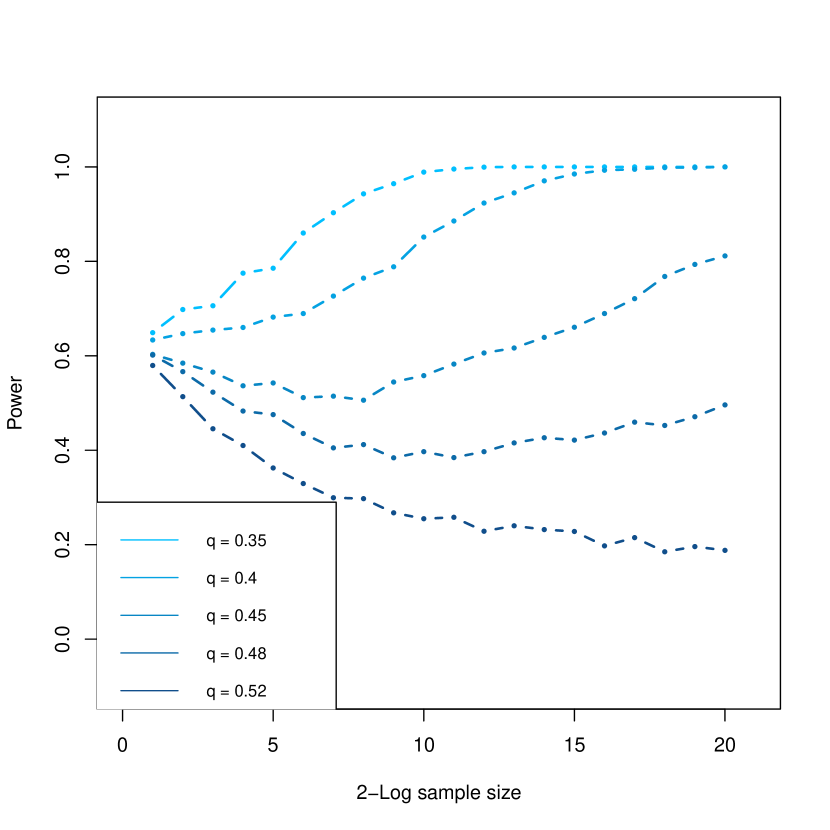
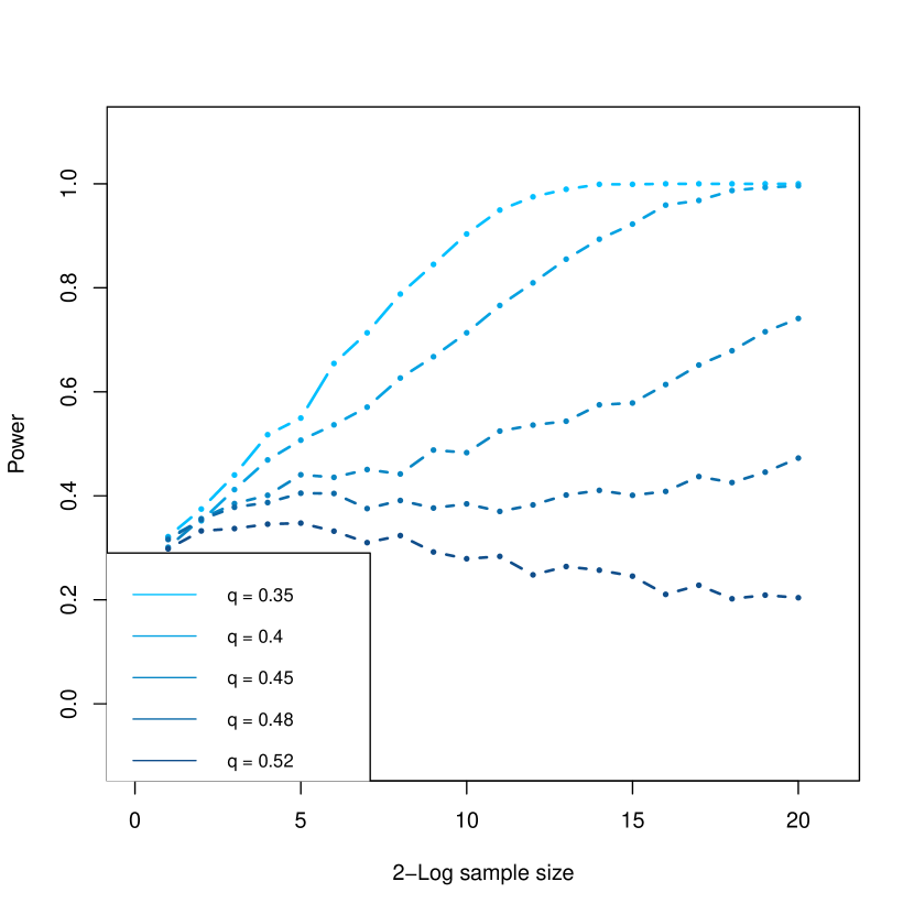
Below we present simulation results under the two settings considered in Example 4.3. The confidence level will be taken as . The power of the LRT in both the simulations below is calculated using an average of replications.
- •
-
•
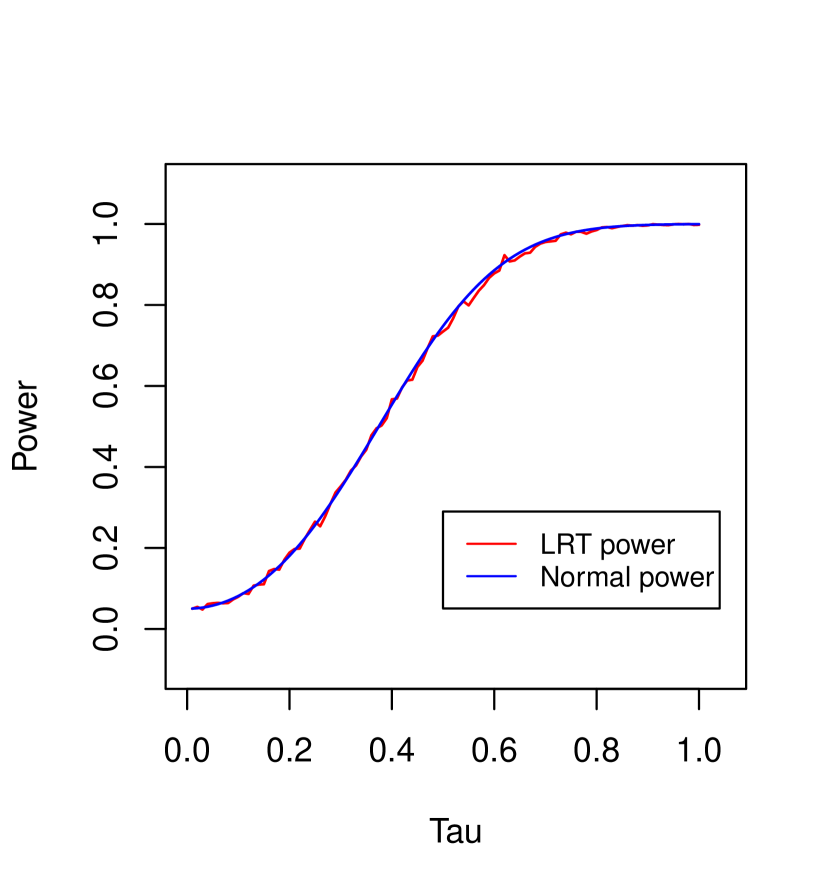
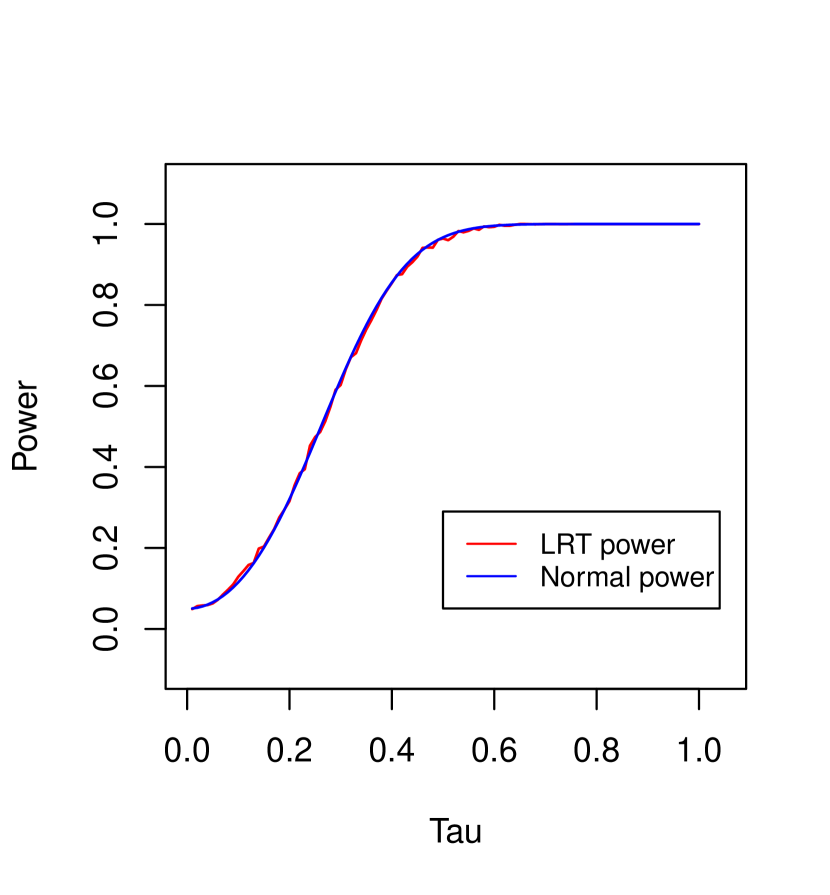
In Figure 2, we fix , , and examine the validity of the normal power expansion (3.14) in Theorem 3.9 along the alternatives considered in Example 4.3 with . Formally, we consider two power curves: (i) the power of the LRT, i.e., , (ii) theoretical power given by the normal approximation, i.e., , for alternatives of the form and with the prescribed ’s. Figure 2 clearly shows that the two power curves are very close to each other.
4.1.2. Counter-examples
Let , and for some fixed to be determined. As long as , we have . We also have , and
where is defined in (4.1). Let . Then , , and .
We first present a choice of that leads to an example showing the necessity of (3.5) for the power characterization (3.6).
Example 4.4.
Next we present a choice of that leads to an example showing the necessity of considering two-sided LRT.
4.2. Testing in circular cone
For any , let the -circular cone be defined by
and let . Consider the testing problem (1.2) with and . The circular cone has recently been used in modeling by [Bes06, GGF08]. The following result (see Section 6.2 for a proof) gives the limiting distribution of the LRS and characterizes the power behavior of the LRT in this example.
Theorem 4.6.
-
(1)
Let . There exists some universal constant such that,
Consequently the LRT is asymptotically size with .
-
(2)
-
(a)
For any , the LRT is power consistent under , i.e., , if and only if .
-
(b)
For any , the LRT is power consistent under , i.e., , if and only if or .
Here for any , with denoting the first components of and denoting the last.
-
(a)
Regarding the two cones , [WWG19] showed the following:
-
•
For , an optimally calibrated LRT is powerful for such that . The minimax -separation rate is of the same constant order, so the LRT is minimax optimal.
-
•
For , an optimally calibrated LRT is powerful for such that , while the minimax -separation rate is of constant order, so the LRT is strictly minimax sub-optimal.
Theorem 4.6-(2) is rather interesting compared to the above results of [WWG19]:
-
•
For , Theorem 4.6-(2)(a) shows that the power behavior of LRT is uniform with respect to for . In other words, for any with the LRT is necessarily not powerful.
-
•
For , Theorem 4.6-(2)(b) shows that the only bad alternatives that drive the uniform separation rate in are those lying in the narrow cylinder and , and the LRT will be powerful for points of the form, e.g. as soon as . This is in line with the result of Theorem 4.6-(2)(a), and provides another example where the LRT exhibits non-uniform power behavior with respect to .
Similar to the LRT in the orthant cone, one may easily see that the conservative uniform separation rate (i.e., ) in for fails to detect ‘most’ alternatives where the LRT is powerful, as . In this sense, the minimax sub-optimality of LRT for testing versus is also conservative as the LRT behaves badly for only a few alternatives with large separation rate in .
The phenomenon observed above for the product circular cone can be easily extended as follows. For some positive integer and generic closed convex cones , , let be the associated product cone. Then the LRT for testing versus is power consistent under if and only if
The proof is largely similar to Theorem 4.6-(2)(b) so we omit the details.
4.3. Testing in isotonic regression
Let the monotone cone be defined by
We consider the testing problem (1.2) with using the two-sided LRT (as in (3.11)). The following result (see Section 6.3 for a proof) gives the limiting distribution of the LRS and characterizes the power behavior of the LRT in this example.
Theorem 4.7.
-
(1)
Suppose , and for a universal constant ,
(4.2) Then
Here is a constant depending on only. Consequently the LRT is asymptotically size with .
-
(2)
Let and , where are monotone functions related by for some function with and is bounded away from and . Suppose the first derivatives are bounded away from and and second derivatives are bounded away from . Then the LRT is power consistent under , i.e., , if and only if , if and only if .
A few remarks are in order.
-
•
(Normal approximation) The normal approximation in Theorem 4.7-(1) settles the problem of the limiting distribution for the LRT used in the simulation in [DT01, Section 4]. There the LRT is compared to a goodness-of-fit test based on the central limit theorem for the estimation error of isotonic LSE (cf. [Gro85, GHL99, Dur07]). We note that condition (4.2) on the sequence is equivalent to a bounded first derivative away from and at the function level. This condition is commonly adopted in global CLTs for type losses of isotonic LSEs, cf. [Dur07]. In fact, the condition in [Dur07] is stronger than (4.2) to guarantee a CLT for estimation error of the isotonic LSE.
-
•
(Rate of normal approximation) We conjecture that the error rate in the above normal approximation is optimal based on the following heuristics. Writing as a shorthand for , the LRS can be written, under , as
Under the regularity condition (4.2), the isotonic LSE is localized in the sense that each roughly depends on and only via indices in a local neighborhood of that contains many points. So one may naturally view as roughly a summation of ‘independent’ blocks, each of which roughly has variance of constant order. This naturally leads to the rate in the Berry-Esseen bound of Theorem 4.7-(1). Our Theorem 4.7-(1) formalizes this intuition, but the proof is along a completely different line.
-
•
(Local power analysis) The ‘local alternative’ setting in Theorem 4.7-(2) follows that of [DT01]. In particular, the separation rate in Theorem 4.7-(2) is reminiscent of [DT01, Theorem 3.1]. [DT01] obtained, under similar configurations and regularity conditions, a separation rate for a goodness-of-fit test based on the CLT for the estimation error of the isotonic LSE of order , where is the length of the support of the function . Our results here show that the LRT has a sharp separation rate under the prescribed configuration, which is no worse than the one derived in [DT01] based on estimation error.
In the isotonic regression example above, the main challenge in deriving the normal approximation for is to lower bound the quantity in (3.1). We detail this intermediate result in the following proposition, which may be of independent interest (see Section 6.3 for a proof).
Proposition 4.8.
Under the setting of Theorem 4.7-(1), there exists a small enough constant , depending on only, such that
for for large enough.
The above proposition is proved via exploiting the min-max representation of the isotonic LSE, a property not shared by general shape-constrained LSEs. We conjecture that results analogous to Theorem 4.7 hold for the general -monotone cone , to be formally defined in Section 4.5, but an analogue to Proposition 4.8 above is not yet available for general .
4.4. Testing in Lasso
Consider the linear regression model
where is a fixed design matrix with and full column rank. Let be the Gram matrix. Let be the ordinary LSE, be the constrained Lasso solution defined as
| (4.3) |
and . The setting here fits into our general framework by letting
and . Note that we do not impose sparsity of here. We will be interested in the testing problem (1.2), i.e., versus , where with . Such a goodness-of-fit test and the related problem of constructing confidence sets for the Lasso estimator has previously been studied in [VV10, CL11, NvdG13, SB18]. In the following, we use the two-sided LRT (as in (3.11)) to test (1.2) and study its power characterization (see Section 6.4 for a proof).
Theorem 4.9.
Suppose . For , let
-
(1)
There exists a universal constant such that, for ,
Consequently the LRT is asymptotically size with , provided that .
-
(2)
Suppose . For any , the LRT is power consistent, i.e., , if and only if .
The proof of Theorem 4.9 relies on the following proposition, which may be of independent interest (see Section 6.4 for a proof).
Proposition 4.10.
The following hold:
-
(1)
.
-
(2)
For any , .
-
(3)
For any , .
Here is an absolute constant.
The proof of the above proposition makes essential use of an explicit representation of the Jacobian derived in [Kat09], which complements its analogues for Lasso in the penalized form derived in [ZHT07, TT12].
Remark 4.11.
A few remarks are in order.
-
(1)
(Choice of ) To apply Theorem 4.9, we need to control the probability term for a generic . This can be done via the following exponential inequality (see Lemma 6.3): for any ,
Here is a universal constant and is the smallest eigenvalue of . Therefore, for any choice of the tuning parameter satisfying
(4.4) for a large enough constant , we have uniformly in . Hence Theorem 4.9 yields that the LRT is asymptotically size and power consistent for all such prescribed ’s if and only if . To get some intuition for this result, for the tuning parameters satisfying (4.4) above, the proof of Proposition 4.10 shows that the Jacobian of (cf. Equation (6.14)) is close to that of the least squares estimator with high probability. From this perspective, the separation rate is quite natural under (4.4) in view of Proposition 3.6 with in the current setting.
-
(2)
(Lasso in penalized form) Theorem 4.9 is applicable for Lasso in its constrained form as defined in (4.3). The penalized form of Lasso
(4.5) however, does not fit into our general testing framework (1.2), and therefore there is no natural associated ‘likelihood ratio test’. An interesting problem is to study the behavior of the statistic defined in (1.1) with replaced by the penalized Lasso estimator . The major hurdle here is to, as in Proposition 4.10-(1), evaluate a lower bound for the Frobenius norm of the the expected Jacobian (see e.g. [BZ21, Proposition 3.10]), where is the (random) support of . Although the penalized form (4.5) is known to be ‘equivalent’ to the constrained form (4.3) in that for each given , there exists some data-dependent such that , due to the random correspondence of and , the techniques used to prove Proposition 4.10 do not translate to a lower bound for . We leave this for a future study.
4.5. Testing parametric assumptions versus shape-constrained alternatives
For fixed and , and consider the testing problem
| (4.6) |
Here and , with denoting the difference operator defined by , and with compositions. It can be readily verified that is a subspace of dimension , is a closed and convex cone, and . Hence (4.6) is a special case of the general testing problem (1.10).
Testing a parametric model against a nonparametric alternative has previously been studied in [CKWY88, ES90, AB93, HM93, Stu97, FH01, GL05, CS10, NVK10, SM17] among which the shape-constrained alternatives in (4.6) are sometimes preferred since the model fits therein usually do not involve the choice of tuning parameters. In particular:
The above two settings have previously been considered in [Bar59a, Bar59b, RWD88, SM17].
Theorem 4.12.
The key step in the proof of Theorem 4.12 (proved in Section 6.5) is to obtain the correct order of the statistical dimension . The discrepancy between and in claim (1) is due to the fact that while a universal upper bound of the order can be proved for any fixed , only a lower bound of the order can be proved for . We conjecture that the correct order of should be for all fixed .
5. Proofs of results in Section 3
5.1. Proof of Theorem 3.1
We need the following proposition, which can be proved using techniques similar to [GNP17, Theorem 2.1]. We provide the details of its proof in Appendix A.2 for the convenience of the reader.
Proposition 5.1.
The next lemma provides a lower bound for the variance of , where the absolute continuity of is valid up to its first derivatives. The proof is based on Fourier analysis in the Gaussian space in the spirit of [NP12, Proposition 1.5.1].
Lemma 5.2.
Let be such that are absolutely continuous and have sub-exponential growth at . Then
Proof.
We only need to verify the above claimed inequality for . Let be the Hermite polynomial of order . For a multi-index and , let . Then is a complete orthogonal basis of , where is the standard Gaussian measure on . On the other hand, the absolute continuity and growth condition on ensures the validity of the following Gaussian integration-by-parts: For all multi-indices such that ,
As , it follows by Plancherel’s theorem that
which equals the right hand side of the claimed inequality. ∎
Proof of Theorem 3.1.
Let
By Lemma 2.1-(1),
Hence
We verify that satisfies the condition of Lemma 5.2. By the above closed-form expression of and , the absolute continuity for holds by noting that is -Lipschitz. On the other hand, as
it follows that have sub-exponential growth at . Now we may apply Lemma 5.2 to see that
as desired. The claim of the theorem now follows from Proposition 5.1. ∎
5.2. Proof of Theorem 3.2
A simple but important observation in the proof of Theorem 3.2 is the following.
Proposition 5.3.
Let
Then for any ,
Proof.
Lemma 5.4.
For any , there exists some such that for all ,
Furthermore, for any compact subset of .
Proof.
We assume without loss of generality. Note that with denoting the d.f. for standard normal,
where depends on only. ∎
Proof of Theorem 3.2.
First note that under the model (1.1), the normalized LRS satisfies the decomposition
| (5.1) |
Using Proposition 5.3, on an event with , we have with defined therein. Then for any ,
| (5.2) | ||||
where
By choosing , we have , so we may apply Lemma 5.4 to see that,
Optimizing , the first two terms in the error bound above can be bounded, up to an absolute constant, by
Next we will obtain a similar upper bound for , but replacing in the above display by . To see this, (5.2) along with
yields that
Similar lower bounds can be derived. Applying the above arguments to the (at most 2) end point(s) of proves the inequality (3.2). Now (1) is a direct consequence of (3.2), while (2) follows by further noting if and only if all limit points of the sequence are contained in . ∎
5.3. Proof of Theorem 3.8
5.4. Proof of Theorem 3.9
First note that we have the decomposition
| (5.3) |
As
we have (as )
Here in the last line of the above display we used that
Let
As by Lemma 2.1-(1),
and hence
Now using the Gaussian concentration inequality for Lipschitz functions, cf. [BLM13, Theorem 5.6], it holds for any that
From here we may conclude (3.14) by using similar arguments as in the proof of Theorem 3.2. Furthermore, by the proof of [WWG19, Lemma E.1], for any , so
The inequality follows as for , and follows as . As , the second inequality (3.15) follows by the bound via Theorem 3.8.
5.5. Proof of Corollary 3.11
We will prove a slightly stronger (than (3.17)) claim that condition (3.19) implies
| (5.4) |
Suppose is greater or equal than times the right hand side of (3.19) for some slowly growing sequence . Then either (i) , or (ii) and . In both cases, we have as there exists some universal constant such that the right hand side of (3.19) is bounded below by . In case (i), using [WWG19, (74a)],
| (5.5) |
as , so (5.4) is verified. In case (ii), we may assume without loss of generality that because otherwise we can follow the same arguments as in the previous case. Then using [WWG19, (74b)] with
we have
as , so (5.4) is verified. The proof is complete. ∎
6. Proofs of results in Section 4
6.1. Proof of Theorem 4.1
Lemma 6.1.
Let be a standard normal random variable. Then for ,
Proof.
The first equality follows as . The second equality follows as . ∎
Proof of Theorem 4.1.
Note that . For , so
As for , and , it follows that
On the other hand, as under the null ,
| (6.1) |
The claim (1) now follows from Theorem 3.1.
For (2), let for
The last equality follows from Lemma 6.1. Hence for all ,
This means that is nonnegative, decreasing with and , and is strictly increasing, concave and bounded on with .
Now note that for any ,
Using the lower bound (6.1) for , and an easy matching upper bound (by e.g. triangle inequality), we have . The condition (3.5) reduces to
| (6.2) |
(6.2) clearly holds for . For , as
the right hand side of (6.2) is bounded from below by
so (6.2) holds. Hence in these two regimes, the claim follows from Theorem 3.2-(2). For , by the decomposition (5.1), the LRT is powerful if and only if , i.e., . The proof is now complete. ∎
6.2. Proof of Theorem 4.6
We write for in the proof for notational convenience.
6.3. Proof of Theorem 4.7
We first prove Proposition 4.8. The following lemma will be used. We present its proof at the end of this subsection.
Lemma 6.2.
Fix . Let and be defined through the following max-min formula for the isotonic LSE:
| (6.3) |
Then there exists some such that for any
Proof of Proposition 4.8.
We write in the proof and for simplicity of notation. Note that . Note that
This implies that
| (6.4) |
We will bound the denominator from above and the numerator from below in the above display separately in the regime , where is a constant to be specified below.
Fix . First we provide an upper bound for the denominator in (6.4). By Lemma 6.2 and using the notation defined therein, there exists some large such that on an event with probability ,
| (6.5) |
and
where is a constant depending on only. Hence integrating the tail leads to the following: for some constant ,
Similarly we can handle the case , so we arrive at
| (6.6) |
for some constant .
Next we provide a lower bound for the numerator of (6.4). On the event (there is nothing special about the constant —a large enough value suffices), we have
where comes from Kolmós-Major-Tusnády strong embedding, and denotes a standard two-sided Brownian motion starting from . The bound for the bias term follows as
| (6.7) |
Now on the event ,
By reflection principle for Brownian motion, for any ,
Let be such that
So for ,
Hence on the event intersected with an event with probability at least ,
where the last inequality follows by choosing for large enough followed by large enough, and on . Combining the above estimates, we see that
on the event intersected with an event with probability at least , when and are chosen large enough, depending on . This event must occur with small enough probability for large in view of (6.5), so we have proved that for large enough and . This means that for for large enough and . Similarly one can handle the regime . In summary, we have proved there exists some such that
| (6.8) |
holds for for large enough. The claim of the proposition now follows by plugging (6.6) and (6.8) into (6.4). ∎
Now we are in position to prove Theorem 4.7.
Proof of Theorem 4.7-(1).
We write in the proof and for simplicity of notation. are shorthanded to if no confusion could arise. For , let and be the maximum integer for which . Clearly for all and . Using the specified in Proposition 4.8, we have
| (6.9) |
On the other hand, by e.g., [Zha02], under the condition of Theorem 4.7, we have
The claim now follows by applying Theorem 3.1 (by ignoring the bias term in the denominator) with the above two displays. ∎
Proof of Theorem 4.7-(2).
Following the notation used in [MW00], let be the greatest convex minorant of , and . Using the same techniques as in [MW00, Theorem 2, Corollary 4] but by performing Taylor expansion to the second order, it can be shown that for all monotone functions with bounded first derivative away from and , and bounded second derivative away from ,
| (6.10) |
Here for a generic , and the term in the above display depends only on the upper and lower bounds for and the upper bound of . Hence for the prescribed ,
On the other hand, for the prescribed , (6.3) provides a lower bound for , while the Gaussian-Poincaré inequality yields a matching upper bound:
Now with , condition (3.5) reduces to
| (6.11) |
where in the last equivalence we used that
By Theorem 3.2-(2), under (6.3) the LRT is power consistent if and only if
| (6.12) |
We have two cases:
To summarize, (6.12) is equivalent to requiring . In this regime (6.3) also holds. The proof is complete. ∎
6.4. Proof of Theorem 4.9
We first prove Proposition 4.10. The following lemma will be useful to control the term therein. We present its proof at the end of this subsection.
Lemma 6.3.
For any with , let . There exists some universal constant such that for ,
Proof of Proposition 4.10.
(1). We will derive an explicit formula for using the results of [Kat09]. First note by the chain rule that
Let . For each , suppose there are faces of of dimension , denoted as . Then we can partition as . Let be a partition of defined as , . Let be the interiors of , respectively. Since is a polyhedron, it follows by [Kat09, Equation (3.6) and Remark 3.3] that when ,
where whose columns are linearly independent and span the tangent space at any point in . Hence on the event ,
which is a projection matrix onto the column space of . In other words, a.e. on ,
| (6.14) |
where
Hence,
and therefore
Here we have used the following:
-
•
In , we apply the estimate
This means for .
-
•
In we use the estimate .
-
•
In the last equality we use .
Thus, claim (1) follows.
(2). Note that
Hence
proving claim (2).
(3). When , as is the projection of onto with respect to , cf. [Kat09, Equation (1.6)]. This means
where
As , by using via the definition of projection, we have
On the other hand, a similar estimate yields
Hence
This completes the proof of claim (3). ∎
Proof of Theorem 4.9.
The first claim follows from Proposition 4.10-(1)(3) and Theorem 3.1 (by ignoring the bias term in the denominator). For the second claim, by Proposition 4.10-(2)(3),
This entails that . Furthermore, using Gaussian-Poincaré inequality along with Proposition 4.10-(1)(3), we have
where the last inequality follows from the condition . This, along with lower bound for derived in Proposition 4.10-(1), yields that . Therefore, under the condition , (3.5) is satisfied automatically, and (3.7) is equivalent to
The proof is complete. ∎
Proof of Lemma 6.3.
Recall that . Note that
with . For any , let be defined as . Then . Hence by Gaussian concentration (cf. [BLM13, Theorem 5.8]), for any ,
| (6.15) |
where . Next we bound and . For , note that
For the mean term, we have . Note that the natural metric induced by the Gaussian process takes the form
and a simple volume estimate yields that
Hence by Dudley’s entropy integral (cf. [GN16, Theorem 2.3.6]),
The claim now follows from (6.15). ∎
6.5. Proof of Theorem 4.12
By definition of , we have . We will now show that
| (6.16) |
where only depends on .
We first prove the upper bound in (6.16) by induction. The baseline case follows by [ALMT14, Equation (D.12)]. Suppose the claim holds for some . For , note that where contains all such that is -monotone, and is -monotone. Hence for any , it follows by [ALMT14, Proposition 3.1] that
where the second inequality follows by induction. On the other hand, let , then Gaussian concentration (cf. [BLM13, Theorem 5.8]) entails that for any ,
Hence, using the induction hypothesis and the union bound, it holds w.p. at least that
Now the bound for follows by integrating the tail.
Next we prove the lower bound in (6.16) for . By Sudakov’s minorization (cf. [GN16, Theorem 2.4.12]), we have
where is the maximal -packing number of set with respect to the metric . By taking to be small enough, the construction in [SHH20, Theorem 3.4] yields an -packing set of cardinality of the order . This completes the lower bound proof.
Appendix A Additional proofs
A.1. Proof of Lemma 2.4
We provide the proof for (1)-(2) assuming is a polyhedral cone. The claim for a general convex cone follows from polyhedral approximation [MT14, Section 7.3].
(1) As , we have .
(2) The claim is proved in [MT14, Proposition 4.4] using the ‘Master Steiner formula’, cf. [MT14, Theorem 3.1], which is a restatement of the chi-bar squared distribution. Below we provide a simple alternative proof of this claim using Gaussian integration-by-parts only.
By expanding and noting that ,
The last equality follows from Gaussian integration-by-parts: (i) (see e.g., [Ste81, Theorem 3], or [BZ21, Theorem 2.1]) and (ii) [BZ21, Equation (2.4)]. Note that (i) using the fact is a cone and Lemma 2.1-(1), and (ii) using the fact that when is polyhedral, is a.e. a projection matrix (cf. [Kat09, Remark 3.3]). Finally using that to conclude.
A.2. Proof of Proposition 5.1
Recall the following second-order Poincaré inequality due to [Cha09].
Lemma A.1 (Second-order Poincaré inequality).
Let be an -dimensional standard normal random vector. Let be absolute continuous such that and its derivatives have sub-exponential growth at . Let be an independent copy of . Define by
Then with ,
Proof.
Let , and . Then [Cha09, Lemma 5.3] says that
The claim follows by the invariance of the total variation metric by translation and scaling. ∎
Proof of Proposition 5.1.
For any fixed , let . By Lemma 2.1-(1), we have
To use the second-order Poincaré inequality, let be an independent copy of and , and let
Hence
The terms involved in the integral in are all absolute continuous, so we may continue to use Gaussian-Poincaré inequality:
| (by Jensen’s inequality applied to the measure ) | ||
Here in the last inequality we used that . Now using that has the same distribution as for each , we arrive at
The claim now follows from the second-order Poincaré inequality in Lemma A.1. ∎
Acknowledgments
The authors would like to thank two referees and an Associate Editor for their helpful comments and suggestions that significantly improved the exposition of the paper.
References
- [AB93] Adelchi Azzalini and Adrian Bowman, On the use of nonparametric regression for checking linear relationships, J. Roy. Statist. Soc. Ser. B 55 (1993), no. 2, 549–557.
- [ACCP11] Ery Arias-Castro, Emmanuel J. Candès, and Yaniv Plan, Global testing under sparse alternatives: ANOVA, multiple comparisons and the higher criticism, Ann. Statist. 39 (2011), no. 5, 2533–2556.
- [ALMT14] Dennis Amelunxen, Martin Lotz, Michael B. McCoy, and Joel A. Tropp, Living on the edge: phase transitions in convex programs with random data, Inf. Inference 3 (2014), no. 3, 224–294.
- [Bar59a] D. J. Bartholomew, A test of homogeneity for ordered alternatives, Biometrika 46 (1959), no. 1-2, 36–48.
- [Bar59b] by same author, A test of homogeneity for ordered alternatives. II, Biometrika 46 (1959), 328–335.
- [Bar61a] by same author, Ordered tests in the analysis of variance, Biometrika 48 (1961), 325–332.
- [Bar61b] by same author, A test of homogeneity of means under restricted alternatives, J. Roy. Statist. Soc. Ser. B 23 (1961), 239–281.
- [Bar02] Yannick Baraud, Non-asymptotic minimax rates of testing in signal detection, Bernoulli 8 (2002), no. 5, 577–606.
- [BBBB72] R. E. Barlow, D. J. Bartholomew, J. M. Bremner, and H. D. Brunk, Statistical inference under order restrictions. The theory and application of isotonic regression, John Wiley & Sons, London-New York-Sydney, 1972, Wiley Series in Probability and Mathematical Statistics.
- [Bes06] Olivier Besson, Adaptive detection of a signal whose signature belongs to a cone, Fourth IEEE Workshop on Sensor Array and Multichannel Processing, 2006., IEEE, 2006, pp. 409–413.
- [BHL05] Yannick Baraud, Sylvie Huet, and Béatrice Laurent, Testing convex hypotheses on the mean of a Gaussian vector. Application to testing qualitative hypotheses on a regression function, Ann. Statist. 33 (2005), no. 1, 214–257.
- [BLM13] Stéphane Boucheron, Gábor Lugosi, and Pascal Massart, Concentration inequalities: A nonasymptotic theory of independence, Oxford University Press, Oxford, 2013.
- [Bou03] Olivier Bousquet, Concentration inequalities for sub-additive functions using the entropy method, Stochastic inequalities and applications, Progr. Probab., vol. 56, Birkhäuser, Basel, 2003, pp. 213–247.
- [BZ21] Pierre C Bellec and Cun-Hui Zhang, Second order stein: Sure for sure and other applications in high-dimensional inference, Ann. Statist. (to appear). Available at arXiv:1811.04121 (2021).
- [Car15] Alexandra Carpentier, Testing the regularity of a smooth signal, Bernoulli 21 (2015), no. 1, 465–488.
- [CCC+19] Alexandra Carpentier, Olivier Collier, Laëtitia Comminges, Alexandre B Tsybakov, and Yu Wang, Minimax rate of testing in sparse linear regression, Automation and Remote Control 80 (2019), no. 10, 1817–1834.
- [CCC+20] Alexandra Carpentier, Olivier Collier, Laetitia Comminges, Alexandre B Tsybakov, and Yuhao Wang, Estimation of the -norm and testing in sparse linear regression with unknown variance, arXiv preprint arXiv:2010.13679 (2020).
- [CCT17] Olivier Collier, Laëtitia Comminges, and Alexandre B. Tsybakov, Minimax estimation of linear and quadratic functionals on sparsity classes, Ann. Statist. 45 (2017), no. 3, 923–958.
- [CD13] Laëtitia Comminges and Arnak S. Dalalyan, Minimax testing of a composite null hypothesis defined via a quadratic functional in the model of regression, Electron. J. Stat. 7 (2013), 146–190.
- [CGS15] Sabyasachi Chatterjee, Adityanand Guntuboyina, and Bodhisattva Sen, On risk bounds in isotonic and other shape restricted regression problems, Ann. Statist. 43 (2015), no. 4, 1774–1800.
- [Cha09] Sourav Chatterjee, Fluctuations of eigenvalues and second order Poincaré inequalities, Probab. Theory Related Fields 143 (2009), no. 1-2, 1–40.
- [Cha14] by same author, A new perspective on least squares under convex constraint, Ann. Statist. 42 (2014), no. 6, 2340–2381.
- [Che54] Herman Chernoff, On the distribution of the likelihood ratio, Ann. Math. Statistics 25 (1954), 573–578.
- [CKWY88] Dennis Cox, Eunmee Koh, Grace Wahba, and Brian S. Yandell, Testing the (parametric) null model hypothesis in (semiparametric) partial and generalized spline models, Ann. Statist. 16 (1988), no. 1, 113–119.
- [CL11] A. Chatterjee and S. N. Lahiri, Bootstrapping lasso estimators, J. Amer. Statist. Assoc. 106 (2011), no. 494, 608–625.
- [CS10] Ronald Christensen and Siu Kei Sun, Alternative goodness-of-fit tests for linear models, J. Amer. Statist. Assoc. 105 (2010), no. 489, 291–301.
- [CV19] Alexandra Carpentier and Nicolas Verzelen, Optimal sparsity testing in linear regression model, arXiv preprint arXiv:1901.08802 (2019).
- [DJ04] David Donoho and Jiashun Jin, Higher criticism for detecting sparse heterogeneous mixtures, Ann. Statist. 32 (2004), no. 3, 962–994.
- [DT01] Cécile Durot and Anne-Sophie Tocquet, Goodness of fit test for isotonic regression, ESAIM Probab. Statist. 5 (2001), 119–140.
- [Dur07] Cécile Durot, On the -error of monotonicity constrained estimators, Ann. Statist. 35 (2007), no. 3, 1080–1104.
- [Dyk91] Richard Dykstra, Asymptotic normality for chi-bar-square distributions, Canad. J. Statist. 19 (1991), no. 3, 297–306.
- [ES90] R. L. Eubank and C. H. Spiegelman, Testing the goodness of fit of a linear model via nonparametric regression techniques, J. Amer. Statist. Assoc. 85 (1990), no. 410, 387–392.
- [FH01] Jianqing Fan and Li-Shan Huang, Goodness-of-fit tests for parametric regression models, J. Amer. Statist. Assoc. 96 (2001), no. 454, 640–652.
- [GGF08] Maria Greco, Fulvio Gini, and Alfonso Farina, Radar detection and classification of jamming signals belonging to a cone class, IEEE transactions on signal processing 56 (2008), no. 5, 1984–1993.
- [GHL99] Piet Groeneboom, Gerard Hooghiemstra, and Hendrik P. Lopuhaä, Asymptotic normality of the error of the Grenander estimator, Ann. Statist. 27 (1999), no. 4, 1316–1347.
- [GL05] Emmanuel Guerre and Pascal Lavergne, Data-driven rate-optimal specification testing in regression models, Ann. Statist. 33 (2005), no. 2, 840–870.
- [GN16] Evarist Giné and Richard Nickl, Mathematical foundations of infinite-dimensional statistical models, Cambridge Series in Statistical and Probabilistic Mathematics, [40], Cambridge University Press, New York, 2016.
- [GNP17] Larry Goldstein, Ivan Nourdin, and Giovanni Peccati, Gaussian phase transitions and conic intrinsic volumes: Steining the Steiner formula, Ann. Appl. Probab. 27 (2017), no. 1, 1–47.
- [Gro85] Piet Groeneboom, Estimating a monotone density, Proceedings of the Berkeley conference in honor of Jerzy Neyman and Jack Kiefer, Vol. II (Berkeley, Calif., 1983), Wadsworth Statist./Probab. Ser., Wadsworth, Belmont, CA, 1985, pp. 539–555.
- [GS18] Adityanand Guntuboyina and Bodhisattva Sen, Nonparametric shape-restricted regression, Statist. Sci. 33 (2018), no. 4, 568–594.
- [HJS21] Qiyang Han, Tiefeng Jiang, and Yandi Shen, A general method for power analysis in testing high dimensional covariance matrices, arXiv preprint arXiv:2101.11086 (2021).
- [HM93] W. Härdle and E. Mammen, Comparing nonparametric versus parametric regression fits, Ann. Statist. 21 (1993), no. 4, 1926–1947.
- [HWCS19] Qiyang Han, Tengyao Wang, Sabyasachi Chatterjee, and Richard J. Samworth, Isotonic regression in general dimensions, Ann. Statist. 47 (2019), no. 5, 2440–2471.
- [HZ19] Qiyang Han and Cun-Hui Zhang, Limit distribution theory for block estimators in multiple isotonic regression, Ann. Statist. (to appear). Available at arXiv:1905.12825 (2019+).
- [IS03] Yu. I. Ingster and I. A. Suslina, Nonparametric goodness-of-fit testing under Gaussian models, Lecture Notes in Statistics, vol. 169, Springer-Verlag, New York, 2003.
- [ITV10] Yuri I. Ingster, Alexandre B. Tsybakov, and Nicolas Verzelen, Detection boundary in sparse regression, Electron. J. Stat. 4 (2010), 1476–1526.
- [JN02] Anatoli Juditsky and Arkadi Nemirovski, On nonparametric tests of positivity/monotonicity/convexity, Ann. Statist. 30 (2002), no. 2, 498–527.
- [Kat09] Kengo Kato, On the degrees of freedom in shrinkage estimation, J. Multivariate Anal. 100 (2009), no. 7, 1338–1352.
- [KC75] Akio Kudô and Jae Rong Choi, A generalized multivariate analogue of the one sided test, Mem. Fac. Sci. Kyushu Univ. Ser. A 29 (1975), no. 2, 303–328.
- [KGGS20] Gil Kur, Fuchang Gao, Adityanand Guntuboyina, and Bodhisattva Sen, Convex regression in multidimensions: Suboptimality of least squares estimators, arXiv preprint arXiv:2006.02044 (2020).
- [Kud63] Akio Kudô, A multivariate analogue of the one-sided test, Biometrika 50 (1963), 403–418.
- [Mey03] Mary C. Meyer, A test for linear versus convex regression function using shape-restricted regression, Biometrika 90 (2003), no. 1, 223–232.
- [MRS92a] J. A. Menéndez, C. Rueda, and B. Salvador, Dominance of likelihood ratio tests under cone constraints, Ann. Statist. 20 (1992), no. 4, 2087–2099.
- [MRS92b] by same author, Testing nonoblique hypotheses, Comm. Statist. Theory Methods 21 (1992), no. 2, 471–484.
- [MS91] J. A. Menéndez and B. Salvador, Anomalies of the likelihood ratio tests for testing restricted hypotheses, Ann. Statist. 19 (1991), no. 2, 889–898.
- [MS20] Rajarshi Mukherjee and Subhabrata Sen, On minimax exponents of sparse testing, arXiv preprint arXiv:2003.00570 (2020).
- [MT14] Michael B. McCoy and Joel A. Tropp, From Steiner formulas for cones to concentration of intrinsic volumes, Discrete Comput. Geom. 51 (2014), no. 4, 926–963.
- [MW00] Mary Meyer and Michael Woodroofe, On the degrees of freedom in shape-restricted regression, Ann. Statist. 28 (2000), no. 4, 1083–1104.
- [NP12] Ivan Nourdin and Giovanni Peccati, Normal approximations with Malliavin calculus, Cambridge Tracts in Mathematics, vol. 192, Cambridge University Press, Cambridge, 2012, From Stein’s method to universality.
- [NvdG13] Richard Nickl and Sara van de Geer, Confidence sets in sparse regression, Ann. Statist. 41 (2013), no. 6, 2852–2876.
- [NVK10] Natalie Neumeyer and Ingrid Van Keilegom, Estimating the error distribution in nonparametric multiple regression with applications to model testing, J. Multivariate Anal. 101 (2010), no. 5, 1067–1078.
- [RLN86] Richard F. Raubertas, Chu-In Charles Lee, and Erik V. Nordheim, Hypothesis tests for normal means constrained by linear inequalities, Comm. Statist. A—Theory Methods 15 (1986), no. 9, 2809–2833.
- [Roc97] R. Tyrrell Rockafellar, Convex Analysis, Princeton Landmarks in Mathematics, Princeton University Press, Princeton, NJ, 1997, Reprint of the 1970 original, Princeton Paperbacks.
- [RW78] Tim Robertson and Edward J. Wegman, Likelihood ratio tests for order restrictions in exponential families, Ann. Statist. 6 (1978), no. 3, 485–505.
- [RWD88] Tim Robertson, F. T. Wright, and R. L. Dykstra, Order restricted statistical inference, Wiley Series in Probability and Mathematical Statistics: Probability and Mathematical Statistics, John Wiley & Sons, Ltd., Chichester, 1988.
- [SB18] Rajen D. Shah and Peter Bühlmann, Goodness-of-fit tests for high dimensional linear models, J. R. Stat. Soc. Ser. B. Stat. Methodol. 80 (2018), no. 1, 113–135.
- [Sha85] Alexander Shapiro, Asymptotic distribution of test statistics in the analysis of moment structures under inequality constraints, Biometrika 72 (1985), no. 1, 133–144.
- [Sha88] A. Shapiro, Towards a unified theory of inequality constrained testing in multivariate analysis, Internat. Statist. Rev. 56 (1988), no. 1, 49–62.
- [SHH20] Yandi Shen, Qiyang Han, and Fang Han, On a phase transition in general order spline regression, arXiv preprint arXiv:2004.10922 (2020).
- [SM17] Bodhisattva Sen and Mary Meyer, Testing against a linear regression model using ideas from shape-restricted estimation, J. R. Stat. Soc. Ser. B. Stat. Methodol. 79 (2017), no. 2, 423–448.
- [Ste81] Charles M. Stein, Estimation of the mean of a multivariate normal distribution, Ann. Statist. 9 (1981), no. 6, 1135–1151.
- [Stu97] Winfried Stute, Nonparametric model checks for regression, Ann. Statist. 25 (1997), no. 2, 613–641.
- [Tib96] Robert Tibshirani, Regression shrinkage and selection via the lasso, J. Roy. Statist. Soc. Ser. B 58 (1996), no. 1, 267–288.
- [TT12] Ryan J. Tibshirani and Jonathan Taylor, Degrees of freedom in lasso problems, Ann. Statist. 40 (2012), no. 2, 1198–1232.
- [vdV98] Aad van der Vaart, Asymptotic Statistics, Cambridge Series in Statistical and Probabilistic Mathematics, vol. 3, Cambridge University Press, Cambridge, 1998.
- [vdV02] by same author, Semiparametric statistics, Lectures on probability theory and statistics (Saint-Flour, 1999), Lecture Notes in Math., vol. 1781, Springer, Berlin, 2002, pp. 331–457.
- [Ver12] Nicolas Verzelen, Minimax risks for sparse regressions: ultra-high dimensional phenomenons, Electron. J. Stat. 6 (2012), 38–90.
- [VV10] Nicolas Verzelen and Fanny Villers, Goodness-of-fit tests for high-dimensional Gaussian linear models, Ann. Statist. 38 (2010), no. 2, 704–752.
- [WR84] Giles Warrack and Tim Robertson, A likelihood ratio test regarding two nested but oblique order-restricted hypotheses, J. Amer. Statist. Assoc. 79 (1984), no. 388, 881–886.
- [WWG19] Yuting Wei, Martin J. Wainwright, and Adityanand Guntuboyina, The geometry of hypothesis testing over convex cones: generalized likelihood ratio tests and minimax radii, Ann. Statist. 47 (2019), no. 2, 994–1024.
- [Zha02] Cun-Hui Zhang, Risk bounds in isotonic regression, Ann. Statist. 30 (2002), no. 2, 528–555.
- [ZHT07] Hui Zou, Trevor Hastie, and Robert Tibshirani, On the “degrees of freedom” of the lasso, Ann. Statist. 35 (2007), no. 5, 2173–2192.