Hierarchical Position Embedding of Graphs with Landmarks and Clustering for Link Prediction
Abstract.
Learning positional information of nodes in a graph is important for link prediction tasks. We propose a representation of positional information using representative nodes called landmarks. A small number of nodes with high degree centrality are selected as landmarks which serve as reference points for the nodes’ positions. We justify this selection strategy for well-known random graph models and derive closed-form bounds on the average path lengths involving landmarks. In a model for power-law graphs, we prove that landmarks provide asymptotically exact information on inter-node distances. We apply theoretical insights to real-world graphs and propose Hierarchical Position embedding with Landmarks and Clustering (HPLC). HPLC combines landmark selection and graph clustering, i.e., the graph is partitioned into densely connected clusters in which nodes with the highest degree are selected as landmarks. HPLC leverages the positional information of nodes based on landmarks at various levels of hierarchy such as nodes’ distances to landmarks, inter-landmark distances and hierarchical grouping of clusters. Experiments show that HPLC achieves state-of-the-art performances of link prediction on various datasets in terms of HIT@K, MRR, and AUC. The code is available at https://github.com/kmswin1/HPLC.
1. Introduction
Graph Neural Networks are foundational tools for various graph related tasks such as node classification (Gilmer et al., 2017; Kipf and Welling, 2017; Hamilton et al., 2017; Veličković et al., 2018), link prediction (Adamic and Adar, 2003; Kipf and Welling, 2016; Zhang and Chen, 2018), graph classification (Xu et al., 2019), and graph clustering (Parés et al., 2017). In this paper, we focus on the task of link prediction using GNNs.
Message passing GNNs (MPGNNs) (Gilmer et al., 2017; Kipf and Welling, 2017; Hamilton et al., 2017; Veličković et al., 2018) have been successful in learning structural node representations through neighborhood aggregation. However, standard MPGNNs achieved subpar performances on link prediction tasks due to their inability to distinguish isomorphic nodes. In order to tackle isomorphism, subgraph-based methods (Zhang and Chen, 2018; Pan et al., 2022) were proposed for link prediction based on dynamic node embeddings from enclosing subgraphs. Labeling methods (Li et al., 2020; Zhang et al., 2021) assign node labels to identify each node via hashing or aggregation functions. An important line of research is the position-based methods (You et al., 2019; Dwivedi et al., 2020; Kreuzer et al., 2021; Wang et al., 2022) which propose to learn and utilize the positional information of nodes.
The positional information of nodes is useful for link prediction because, e.g., isomorphic nodes can be distinguished by their positions, and the link formation between a node pair may be related to their relative distance (Srinivasan and Ribeiro, 2020). The position of a node can be defined as its distances relative to other nodes. A relevant result by Bourgain (Bourgain, 1985) states that inter-node distances can be embedded into Euclidean space with small errors. Linial (Linial et al., 1995) and P-GNN (You et al., 2019) focus on constructing Bourgain’s embeddings based on the nodes’ distances to random node sets. Another line of positional encoding used the eigenvectors of graph Laplacian (Dwivedi and Bresson, 2021; Kreuzer et al., 2021) based on spectral graph theory. However, the aforementioned methods have convergence issues and may not scale well for large or dense graphs (Wang et al., 2022). For example, Laplacian methods have stability issues (Wang et al., 2022) and may not outperform methods based on structural features (Zhang and Chen, 2018). Thus, there is significant room for improving both performance and scalability of positional node embedding for link prediction.
In this paper, we propose an effective and efficient representation of the positional information of nodes. We select a small number of representative nodes called landmarks and impose hierarchy on the graph by associating each node with a landmark. Each node computes distances to the landmarks, and each landmark computes distances to other landmarks. Such distance information is combined so as to represent nodes’ positional information. Importantly, we select landmarks and organize the graph in a principled way, unlike previous methods using random selection, e.g., (Bourgain, 1985; Linial et al., 1995; You et al., 2019).
The key question is how to select landmarks. We advocate the selection based on degree centrality which is motivated from the theory of network science. In network models with preferential attachment (PA), nodes with high degrees called hubs are likely to emerge (Barabási and Albert, 1999). PA is a process such that, if a new node joins the graph, it is more likely to connect to nodes with higher degrees. PA induces the power-law distribution of node degrees, and the network exhibits scale-free property (Barabási and Albert, 1999). Hubs are abundant in social/citation networks and World Wide Web, and play a central role in characterizing the network.
We provide a theoretical justification of landmark selection based on degree centrality for a well-known class of random graphs (Erdős et al., 1960; Barabási and Albert, 1999). We show that the inter-node distances are well-represented by the detour via landmarks. In networks with preferential attachment, we show that the strategy of choosing high-degree nodes as landmarks is asymptotically optimal in the following sense: the minimum distance among the detours via landmarks is asymptotically equal to the shortest-path distance. We show even a small number of landmarks relative to network size, e.g., , suffice to achieve optimality. This proves that the hub-type landmarks offer short paths to nodes, manifesting small-world phenomenon (Watts and Strogatz, 1998; Barabási and Albert, 1999). In addition, we show that in models where hubs are absent, one can reduce the detour distance by selecting a higher number of landmarks.
Motivated by the theory, we propose Hierarchical Position embedding with Landmarks and Clustering (HPLC). HPLC partitions a graph into clusters which are locally dense, and appoints the node with the highest degree in the cluster as the landmark. Our intention is to bridge gap between theory and practice: hubs may not be present in real-world graphs. Thus, it is important to distribute the landmarks evenly over the graph through clustering, so that nodes can access nearby/local landmarks. Next, we form a graph of higher hierarchy, i.e., the graph of landmarks, and compute its Laplacian encoding based on the inter-landmark distances. The encoding is assigned as a membership to the nodes belonging to the cluster so as to learn positional features at the cluster level. We further optimize our model using the encoding based on hierarchical grouping of clusters. The computation of HPLC can be mainly done during preprocessing, incurring low computational costs. Our experiments on 7 datasets with 16 baseline methods show that HPLC achieves state-of-the-art performances, demonstrating its effectiveness especially over prior position-/distance-based methods.
Our contributions are summarized as follows: 1) we propose HPLC, a highly efficient algorithm for link prediction using hierarchical position embedding based on landmarks combined with graph clustering; 2) building upon network science, we derive closed-form bounds on average path lengths via detours for well-known random graphs which, to our belief, are important theoretical findings; 3) we conduct extensive experiments to show that HPLC achieves state-of-the-art performances in most cases.
2. Random Graphs with Landmarks
2.1. Notation
We consider undirected graph where and denote the set of vertices and edges, respectively. Let denote the number of nodes, or . denotes the adjacency matrix of . denotes the geodesic (shortest-path) distance between and . Node attributes are defined as where denotes the feature vector of node . We consider methods of embedding into the latent space as vectors . We study the node-pair-level task of estimating the link probability between and from and .
2.2. Representation of Positions using Landmarks
The distances between nodes provide rich information on the graph structures. For example, a connected and undirected graph can be represented by a finite metric space with its vertex set and the inter-node distances, and the position of a node can be defined as its relative distances to other nodes. However, computing and storing shortest paths for all pairs of nodes incur high complexity.
Instead, we select a small number of representative nodes called landmarks. The landmarks are denoted by where denotes the number of landmarks. For node , we define -tuple of distances to landmarks as distance vector (DV):
can be used to represent the (approximate) position of node . If the positions of and are to be used for link prediction, one can combine and (or the embeddings thereof) to estimate the probability of link formation.
The key question is, how much information has on the inter-node distances within the graph, so that positional information can be (approximately) recovered from . For example, from triangle inequality, the distance between nodes and are bounded as
which states that the detour via landmarks, i.e., from to to , is longer than , but the shortest detour, or the minimum component of , may provide a good estimate of . Indeed, it was empirically shown that the shortest detour via base nodes (landmarks) can be an excellent estimate of distances in Internet (Ng and Zhang, 2002).
We examine the achievable accuracy of distance estimates based on the detours via landmarks. Previous works on distance estimates using auxiliary nodes relied on heuristics (Potamias et al., 2009) or complex algorithms for arbitrary graphs (Linial et al., 1995; You et al., 2019). However, real-world graphs have structure, e.g., preferential attachment or certain distribution of node degrees. Presumably, one can exploit such structure to devise efficient algorithms. The key design questions are: how to select good landmarks, and how many of them? Drawing upon the theory of network science, we analyze a well-known class of random graphs, derive the detour distances via landmarks, and glean design insights from the analysis.
| (1) |
| (2) |
2.3. Path lengths via Landmarks in random graphs
The framework by (Fronczak et al., 2004) provides a useful tool for analyzing path lengths for a wide range of classes of random graphs as follows. Consider a random graph where the probability of the existence of an edge for node and denoted by is given by
| (3) |
where is tag information of node , e.g., the connectivity or degree of the node, and is a parameter depending on the network model. From the continuum approximation (Albert and Barabási, 2002) for large graphs, tag information is regarded as a continuous random variable (RV) with distribution . For some measurable function , let denote the expectation of of a node chosen at random, and denote the expectation of of landmarks chosen under some distribution .
Theorem 1.
Let denote the random variable representing the minimum path length from node to among the detours via landmarks. The landmarks are chosen i.i.d. according to distribution . Asymptotically in , is given by (1).
The proof of Theorem 1 is in Appendix A.1. In (1), the design parameters are and which are related to what kind of landmarks are chosen, and how many of them, respectively. Next, we bound the average distance of the shortest detour via landmarks. In what follows, we will assume and as , implying that the number of landmarks is chosen to be not too large compared to .
Theorem 2.
The average distance of the shortest detour via landmarks, denoted by , is bounded above as (2) where is the Euler’s constant.
The proof of Theorem 2 is in Appendix A.2. Next, we apply the results to some well-known models for random graphs.
| (4) |
2.4. Erdős-Rényi Model
The Erdős-Rényi (ER) model (Erdős et al., 1960) is a classical random graph in which every node pair is connected with a common probability. For ER graphs, model parameters and can be set as and respectively, where denotes the mean degree of nodes (Boguná and Pastor-Satorras, 2003). From (3), we have , i.e., the probability of edge formation between any node pair is constant. The node degree follows the Poisson distribution with mean for large .
We apply our analysis to ER graphs as follows. By plugging in the model parameters to (2), the average distance of the shortest detour via landmarks in ER graphs, denoted by , is bounded above as
| (5) |
asymptotically in . Meanwhile, the average inter-node distance in ER graphs denoted by , is given by (Boguná and Pastor-Satorras, 2003; Fronczak et al., 2004)
| (6) |
By comparing (5) and (6), we observe that the detour via landmarks incurs the overhead of at most factor 2. This is because, the nodes in ER graphs appear homogeneous, and thus the path length to and from landmarks are on average similar to the inter-node distance. Thus, the average distance of a detour will be twice the direct distance. However, (5) implies that the minimum detour distance can be reduced by using multiple landmarks. The reduction can be substantial, e.g., if for some , we have, from (5),
For example, selecting landmarks guarantees a 1.5-factor approximation of the shortest path distance. By making close to 0, we get arbitrarily close to the shortest path distance.
Discussion. Due to having Poisson distribution, the degrees in ER graphs are highly concentrated on mean . There seldom are nodes with very large degrees, i.e., most nodes look alike. Thus, the design question should be on how many rather than on what kind of landmarks. We benefit from choosing a large number of landmarks, e.g., . However, there is a trade-off: the computational overhead of managing -dimensional vector will be high.
2.5. Barabási-Albert Model
The Barabási-Albert (BA) model (Barabási and Albert, 1999) generates random graphs with preferential attachment. BA graphs are characterized by continuous growth over time: initially there are nodes, and new nodes arrive to the network over time. Due to preferential attachment, the probability of a newly arriving node connecting to the existing node is proportional to its degree. The probability of an edge in BA graphs is shown to be (Boguná and Pastor-Satorras, 2003)
with and , where is the time of arrival of node . Since the probability of a newly arriving node connecting to node is proportional to , the degree of nodes with large is likely to be high. For large , the distribution of is derived as (Fronczak et al., 2004)
| (7) |
By applying to (2), we bound the average path length with landmarks denoted by as (4). Importantly, unlike ER graphs, there exists a landmark selection strategy which achieves the asymptotically optimal distance, despite using a small number of landmarks relative to the network size.
Theorem 3.
Suppose landmarks are randomly selected from the nodes with top- largest values of . Assume . The average distance of the shortest detour via landmarks, denoted by , is bounded as
| (8) |
asymptotically in .
The proof of Theorem 3 is in Appendix A.3. We claim the optimality of the strategy in Theorem 3 in the following sense. Since is slowly increasing in , e.g., , a feasible strategy for Theorem 3 is to choose landmarks from top– degree nodes. For such , the numerator of the RHS of (8) is for large . Meanwhile, the average length of shortest paths in BA graphs is given by (Cohen and Havlin, 2003)
| (9) |
By comparing (8) and (9), we conclude that is asymptotically equal to . This implies that the shortest detour via landmarks under our strategy has on average the same length as the shortest path in the asymptotic sense.
Discussion. The node degree in BA graphs is known to follow power-law distribution which causes the emergence of hubs. Inter-node distances can be drastically reduced by hubs, known as small-world phenomenon (Barabási and Albert, 1999). We showed that the shortest path is indeed well-approximated by the detour via landmarks with sufficiently high degrees. Importantly, it is achieved with a small number of landmarks, e.g., let in (8).
Summary of Analysis. ER and BA models represent two contrasting cases of degree distributions. The degree distribution of ER graph is highly concentrated, i.e., the variation of node degrees is small, or hubs are absent. By contrast, the degree of BA graphs follows power-law distribution, i.e., the variation of node degree is large, and hubs are present. Our analysis shows that -factor approximation (ER) and asymptotic optimality (BA) are achievable by detour via landmarks. The derived bounds are numerically verified via simulation in Appendix B.

2.6. Design Insights from Theory
The key design questions we would like to address are: what kind of, and how many, landmarks should be selected?
Landmark Selection and Graph Clustering. Theorem 3 states that, one should choose landmarks with sufficiently large , e.g., high-degree nodes. However, such high-degree nodes may not always provide short paths for real-world graphs. For example, suppose all the hubs are located at one end of the network. The nodes at the other end of the network need to make a long detour via landmarks, even in order to reach nodes in local neighborhoods.
In order to better capture local graph structure and evenly distribute landmarks over the graph, we propose to partition the graph into clusters such that the nodes within a cluster tend to be densely connected, i.e., close to one another. Next, we propose to pick the node with the highest degree within each cluster as the landmark, as suggested by the analysis. Each landmark represents the associated cluster, and the distance between nodes can be captured by distance vectors associated with the cluster landmarks. We empirically find that the combination of landmark selection and clustering yields improved results.
Number of Landmarks. Although large appears preferable, our analysis show that does not drastically reduce distances, unless is very large, e.g., . A large number of landmarks can hamper scalability. Thus, we use only a moderate number of landmarks as suggested by the analysis. Indeed, we empirically found that setting suffices to yield good results.
3. Proposed Method
In this section, Hierarchical Position embedding with Landmarks and Clustering (HPLC) is described. The main method combining landmarks and clustering is explained in Sec. 3.1. Additional optimization methods leveraging landmarks and clusters are introduced, which are membership encoding (Sec. 3.2) and cluster-group encoding (Sec. 3.3). An overview of HPLC is depicted in Fig. 1.
3.1. Graph Clustering and Landmark Selection
Graph clustering is a task of partitioning the vertex set into disjoint subsets called clusters, where the nodes within a cluster tend to be densely connected relative to those between clusters (Schaeffer, 2007). We will use FluidC graph clustering algorithm proposed in (Parés et al., 2017) as follows. Suppose we want to partition to clusters. FluidC initially selects random central nodes, assigns each node to clusters , and iteratively assigns nodes to clusters according to the following rule. Node is assigned to cluster such that
| (10) |
where denotes the neighbors of . This assignment rule prefers community candidates of small sizes (denominator), which results in well-balanced cluster sizes. The rule also prefers communities already containing many neighbors of (numerator), which makes clusters locally dense. As a result, FluidC generates densely-connected cohesive clusters of relatively even sizes. In addition, FluidC has complexity , and thus is highly scalable (Parés et al., 2017). Importantly, the number of clusters can be specified beforehand, which is crucial because is a hyperparameter in our method.
For each cluster, we select the node with the highest degree as the landmark, where denotes the landmark of cluster . For node , we compute the distances to landmarks to yield distance vector . Since may be disconnected, we extend the definition of distance such that, in case there exists no path from to , is set to where is the maximum diameter among the connected components. As stated earlier, we set number of clusters where integer is a hyperparameter.
Effect of Clustering on Landmarks. The proposed method first performs clustering, and then selects landmarks based on degree centrality. The analysis in Sec. 2 showed that the nodes with sufficiently high degree centrality should be chosen as landmarks. The question is whether the landmarks chosen after clustering will have sufficiently high degrees.
A supporting argument for incorporating clustering into analysis can be made for BA graphs. Theorem 3 states that, choosing landmarks from top- nodes in degrees is optimal. We show that, landmarks chosen after FluidC clustering are indeed within top- degree centrality through simulation. Table 1 compares the rank of degrees of landmarks selected after FluidC clustering versus the rank of top- degree nodes in BA graphs. We observe that the landmarks selected after clustering have sufficiently large degrees for optimality, i.e., all of their degrees are within top-.
The result can be explained as follows. Power-law graphs are known to have modules which are densely connected subgraphs and are sparsely connected to each other (Goh et al., 2006). A proper clustering algorithm is expected to detect modules. Moreover, each cluster contains a relatively large number of nodes, because the number of clusters is relatively small . Thus, each cluster is likely to contain nodes with sufficiently high degrees which are, according to Theorem 3, good candidates for landmarks.
One can expect similar effects from FluidC clustering for real-world graphs. Given the small number of clusters as input, the algorithm will detect locally dense clusters resulting in landmarks which have high degrees and tend to be evenly distributed over the graph. Thus, landmark selection after clustering can be a good heuristic motivated by the theory.
Network size rank: cluster landmarks rank: top- Fraction of landmarks within rank top- 500 5.02% 6.38% 100% 1000 3.02% 4.37% 100% 2000 1.76% 2.85% 100% 5000 0.90% 1.48% 100%
3.2. Membership Encoding with Graph Laplacian
For the nodes within the same cluster, we augment the nodes’ embeddings with information identifying that they are members of the same community, which we call membership. The membership is extracted from landmarks, and is based on the relative positional information among landmarks. Thus, not only the nodes within the same cluster have the same membership, but also the nodes of neighboring clusters have “similar” membership. The membership of a node is encoded into a membership vector (MV) which is combined with DV in computing the node embeddings.
We consider the graph consisting only of landmark nodes, and use graph Laplacian (Belkin and Niyogi, 2003) to encode their relative positions as follows. The landmark graph uses the edge weight between landmarks and which is set to where denotes normalizing parameter of heat kernel. Let denote the weighted adjacency matrix. The normalized graph Laplacian is given by where degree matrix is given by . The eigenvectors of are used as MVs, i.e., for node , the MV of node , denoted by , is the eigenvector of associated with landmark . MV provides positional information in addition to DV, using the graph of upper hierarchy, i.e., landmarks. We use a random flipping of the signs of eigenvectors to resolve ambiguity (Dwivedi et al., 2020). A problem with Laplacian encoding is the time complexity: one needs the eigendecomposition whose complexity is cubic in network size. Thus, previous approaches had limitations, i.e., used only a subset of eigenspectrum (Dwivedi et al., 2020; Kreuzer et al., 2021). However, in our method, the landmark graph has small size, i.e., . Thus, we can exploit the full eigenspectrum, enabling more accurate representation of landmark graphs.
3.3. Cluster-group Encoding
We propose cluster-group encoding as an additional model optimization as follows. Several neighboring clusters are further grouped into a macro-cluster. The embeddings of nodes in a macro-cluster use an encoder specific to that macro-cluster. The motivation is that, using a separate encoder per local region may facilitate capturing attributes specific to local structures or latent features of the community, which is important for link prediction.
For cluster , let denote the macro-cluster which contains where denote the index of the macro-cluster. The node embedding for node is computed as
where is the input node feature, and are MV and DV, is membership/distance encoder, and denotes concatenation. denotes the encoder specific to macro-cluster . MLPs are used for and . The number of macro-cluster, denoted by , is set such that is a multiple of . Each macro-cluster contains clusters. Cluster-group encoding requires encoders, one per macro-cluster. To limit the model size, we empirically set . For ease of implementation, is first partitioned into macro-clusters, then each macro-cluster is partitioned into clusters. This is simpler than, say, partitioning into (smaller) clusters and grouping them back to macro-clusters.
Next, is input to GNN whose -th layer output is given by
where . HPLC is a plug-in method and thus can be combined with different types of GNNs. The related study is provided in Sec. 7.2. Finally, we concatenate node-pair embeddings and compute scores by where denotes the link prediction score between node and , and is an MLP.
4. Property of HPLC as Node embedding
In (Srinivasan and Ribeiro, 2020), the (positional) node embeddings are formally defined as:
Definition 0.
The node embeddings of a graph with adjacency matrix and input attributes are defined as joint samples of random variables , , where is a -equivariant probability distribution on and , that is, for any permutation
It is argued in (Srinivasan and Ribeiro, 2020) that positional node embeddings are good at link prediction tasks: the positional embeddings preserve the relative positions of nodes, which enables differentiating isomorphic nodes according to their positions and identifying the closeness between nodes. We claim that HPLC qualifies as positional node embeddings according to Definition 1 as follows.
In HPLC, landmark-based distance function, eigenvectors of graph Laplacian with random flipping, and graph clustering method are -equivariant functions of ignoring the node features . The landmark-based distance vectors and its functions clearly satisfy the equivariance property. The eigenvectors of graph Laplacian are permutationally equivariant under the node permutation, i.e., switching of corresponding rows/columns of adjacency matrix. Also, the Laplacian eigenmap can be regarded as a -equivariant function in the sense of expectation, if it is combined with random sign flipping of eigenvectors (Srinivasan and Ribeiro, 2020). In case of multiplicity of eigenvalues, we can slightly perturb the edge weights of landmark graphs to obtain simple eigenvalues (Poignard et al., 2018). The graph clustering in HPLC is a randomized method, because initially central nodes are selected at random. Thus, embedding output of HPLC is a function of , and random noise, which proves our claim that HPLC qualifies as a positional node embedding.
Moreover, HPLC is more expressive than standard message-passing GNNs as follows. HPLC is trained to predict the link between a node pair based on their positional embeddings. The embeddings are learned over the joint distribution of distances from node pairs to common landmarks which are spread out globally over the graph. By contrast, traditional GNNs learn the embeddings based on the marginal distributions of local neighborhoods of node pairs. By a similar argument to Sec. 5.2 of (You et al., 2019), HPLC induces higher mutual information between its embeddings and the target similarity (likelihood of link formation) of node pairs based on positions, and thus has higher expressive power than standard GNNs.
5. Complexity Analysis
5.1. Time Complexity
The time complexity of HPLC is incurred mainly from computing DVs and MVs. We first consider the complexity of computing for all . There are landmarks, and for each landmark, computing the distances from all to the landmark requires using Fibonacci heap. Thus, the overall complexity is . Next, we consider the complexity of computing . We compute Laplacian eigenvectors of landmark graph, where its time complexity is . Importantly, the computation of and can be done during the preprocessing stage.
5.2. Space Complexity
The space complexity of HPLC is mainly from the GNN models for computing the node embeddings. Additional space complexity of HPLC is from the membership/distance encoder which is , and cluster-group encoding which is respectively, where denotes the node feature dimension, denotes the number of macro-clusters, denotes the hidden dimension of , and denotes the hidden dimension of cluster-group encoders.
Overall, the time and space complexity of HPLC is low, and our experiments shows that HPLC handles large or dense graphs well. We also measured the actual resource usage, and the related results are provided in Appendix D.
Baselines Avg. (H.M.) CITATION2 COLLAB DDI PubMed Cora Citeseer Facebook Adamic Adar 65.74 (50.65) 76.12 0.00 53.00 0.00 18.61 0.00 66.89 0.00 77.22 0.00 68.94 0.00 99.41 0.00 MF 54.06 (42.65) 53.08 4.19 38.74 0.30 17.92 3.57 58.18 0.01 51.14 0.01 50.54 0.01 98.80 0.00 Node2Vec 64.01 (51.17) 53.47 0.12 41.36 0.69 21.95 1.58 80.32 0.29 84.49 0.49 80.00 0.68 86.49 4.32 GCN (GAE) 76.35 (66.67) 84.74 0.21 44.14 1.45 37.07 5.07 95.80 0.13 88.68 0.40 85.35 0.60 98.66 0.04 GCN (MLP) 76.48 (67.53) 84.79 0.24 44.29 1.88 39.31 4.87 95.83 0.80 90.25 0.53 81.47 1.40 99.43 0.02 GraphSAGE 78.51 (71.48) 82.64 0.01 48.62 0.87 44.82 7.32 96.58 0.11 90.24 0.34 87.37 1.39 99.29 0.01 GAT - - 44.14 5.95 29.53 5.58 85.55 0.23 82.59 0.14 87.29 0.11 99.37 0.00 JKNet - - 48.84 0.83 57.98 7.68 96.58 0.23 89.05 0.67 88.58 1.78 99.43 0.02 P-GNN - - - 1.14 0.25 87.22 0.51 85.92 0.33 90.25 0.42 93.13 0.21 GTrans+LPE - - 11.19 0.42 9.22 0.20 81.15 0.12 79.31 0.09 77.49 0.02 99.27 0.00 GCN+LPE 74.60 (67.00) 84.85 0.35 49.75 1.35 38.18 7.62 95.50 0.13 76.46 0.15 78.29 0.21 99.17 0.00 GCN+DE 72.48 (60.04) 60.30 0.61 53.44 0.29 26.63 6.82 95.42 0.08 89.51 0.12 86.49 0.11 99.38 0.02 GCN+LRGA 78.42 (74.47) 65.05 0.22 52.21 0.72 62.30 9.12 93.53 0.25 88.83 0.01 87.59 0.03 99.42 0.05 SEAL 77.08 (62.88) 85.26 0.98 53.72 0.95 26.25 8.00 95.86 0.28 92.55 0.50 85.82 0.44 99.60 0.02 NBF-net - - - 4.03 1.32 97.30 0.45 94.12 0.17 92.30 0.23 99.42 0.04 PEG-DW+ 81.67 (75.42) 86.03 0.53 53.70 1.18 47.88 4.56 97.21 0.18 93.12 0.12 94.18 0.18 99.57 0.05 HPLC 85.77 (82.39) 86.15 0.48 56.04 0.28 70.03 7.02 97.38 0.34 94.95 0.18 96.15 0.19 99.69 0.00
6. Experiments
6.1. Experimental setting
Datasets. Experiments were conducted on 7 datasets widely used for evaluating link prediction. For experiments on small graphs, we used PubMed, Cora, Citeseer, and Facebook. For experiments on dense or large graphs, we chose DDI, COLLAB, and CITATION2 provided by OGB (Hu et al., 2020). Detailed statistics and evaluation metrics of the datasets are provided in Table 9 in Appendix E.
Baseline models. We compared HPLC with Adamic Adar (AA) (Adamic and Adar, 2003), Matrix Factorization (MF) (Koren et al., 2009), Node2Vec (Grover and Leskovec, 2016), GCN (Kipf and Welling, 2017), GraphSAGE (Hamilton et al., 2017), GAT (Veličković et al., 2018), P-GNN (You et al., 2019), NBF-net (Zhu et al., 2021), and plug-in type approaches like JKNet (Xu et al., 2018), SEAL (Zhang and Chen, 2018), GCN+DE (Li et al., 2020), GCN+LPE (Dwivedi et al., 2020), GCN+LRGA (Puny et al., 2021), Graph Transformer+LPE (Dwivedi and Bresson, 2021), and PEG-DW+ (Wang et al., 2022). All methods except for AA and GAE are computed by the same decoder, which is a 2-layer MLP. For a fair comparison, we use GCN in most plug-in type approaches: SEAL, GCN+DE, GAE, JKNet, GCN+LRGA, GCN+LPE, and HPLC.
Evaluation metrics. Link prediction was evaluated based on the ranking performance of positive edges in the test data over negative ones. For COLLAB and DDI, we ranked all positive and negative edges in the test data, and computed the ratio of positive edges which are ranked in top-. We did not utilize validation edges for computing node embeddings when we predicted test edges on COLLAB. In CITATION2, we computed all positive and negative edges, and calculated the reverse of the mean rank of positive edges.
Due to high complexity when evaluating SEAL, we only trained 2% of training set edges and evaluated 1% of validation and test set edges respectively, as recommended in the official GitHub of SEAL.
The metrics for DDI, COLLAB and CITATION2 are chosen according to the official OGB settings (Hu et al., 2020). For Cora, Citeseer, PubMed, and Facebook, Area Under ROC Curve (AUC) is used as the metric similar to prior works (Kipf and Welling, 2017; Wang et al., 2022). If applicable, we calculated the average and harmonic mean (HM) of the measurements. HM penalizes the model for very low scores, thus is a useful indicator of robustness.
Hyperparameters. We used GCN as our base GNN encoder.
MLP is used in decoders, except GAE. None of the baseline methods used edge weights. During training, negative edges are randomly sampled at a ratio of 1:1 with positive edges. The details of hyperparameters are provided in Appendix F.
6.2. Results
Experimental results are summarized in Table 2. HPLC outperformed the baselines on most datasets. HPLC achieved large performance gains over GAE combined with GCN on all datasets, which are 88.9% on DDI, 27.0% on COLLAB, 12.7% on Citeseer, 7.1% on Cora, and 1.4% on CITATION2. HPLC showed superior performance over SEAL, achieving gains of 167% on DDI, and 12.0% on Citeseer. We compare HPLC with other distance-based methods. Compared to GCN+DE which encodes distances from a target node set whose representations are to be learned, or to P-GNN which uses distances to random anchor sets, HPLC achieved higher performance gains by a large margin. HPLC outperformed other positional encoding methods, e.g., GCN+LPE, Graph Transformer+LPE, and PEG-DW+. The results show that the proposed landmark-based representation can be effective for estimating the positional information of nodes.
SEAL and NBF-net performed poorly on DDI which is a highly dense graph. Since the nodes of DDI have a large number of neighbors, the enclosing subgraphs are both very dense and large, and the models struggle with learning the representations of local structures or paths between nodes. By contrast, HPLC achieved the best performance on DDI, demonstrating its effectiveness on densely connected graphs.
Finally, we computed the average and harmonic means of performance measurements except for the methods with OOM problems. Although the averages are taken over heterogeneous metrics and thus do not represent specific performance metrics, they are presented for comparison purposes. In summary, HPLC achieved the best average and harmonic mean of performance measurements, demonstrating both its effectiveness and robustness.
7. Ablation study
In this section, we provide the ablation study. Additional ablation studies on graph clustering algorithms and node centrality are provided in Appendix C.
7.1. Model Components
Table 3 shows the performances in the ablation analysis for the model components. The components denoted by“DV”, “CE” and “MV” columns in Table 3 indicate the usage of distance vector, cluster-group encoding and membership vector, respectively. The results show that all of the hierarchical components, i.e., “DV”, “CE” and “MV”, indeed contribute to the performance improvement.
| DV | CE | MV | COLLAB | DDI | PubMed | Cora | Citeseer |
| ✗ | ✗ | ✗ | 44.29 1.88 | 39.31 4.87 | 95.83 0.80 | 90.25 0.53 | 81.43 0.02 |
| ✗ | ✔ | ✗ | 52.64 0.39 | 54.00 8.90 | 95.93 0.19 | 92.21 0.13 | 95.54 0.16 |
| ✗ | ✗ | ✔ | 44.33 0.24 | 41.33 5.82 | 95.92 0.15 | 91.82 0.18 | 94.87 0.12 |
| ✔ | ✗ | ✗ | 53.31 0.62 | 46.86 9.91 | 95.97 0.13 | 92.32 0.25 | 95.13 0.18 |
| ✔ | ✔ | ✗ | 55.56 0.37 | 68.75 7.43 | 96.67 0.18 | 93.94 0.21 | 95.83 0.15 |
| ✔ | ✔ | ✔ | 56.04 0.28 | 70.03 7.02 | 97.38 0.34 | 94.95 0.18 | 96.15 0.19 |
7.2. Combination with various GNNs
HPLC can be combined with different GNN encoders. We experimented the combination with three types of widely-used GNN encoders. Table 4 shows that, HPLC enhances the performance of various types of GNNs.
| Dataset | w/ GraphSAGE | w/ GAT | w/ GCN |
|---|---|---|---|
| PubMed | 96.63 () | 93.18 () | 97.38 () |
| Cora | 96.18 () | 91.93 () | 94.95 () |
| Citeseer | 94.97 () | 94.60 () | 96.15 () |
| 99.48 () | 99.40 () | 99.69 () |
8. Related Work
Link Prediction. Earlier methods for link prediction used heuristics (Adamic and Adar, 2003; Page et al., 1998; Zhou et al., 2009) based on manually designed formulas. GNNs were subsequently applied to the task, e.g., GAE (Kipf and Welling, 2016) is a graph auto-encoder which reconstructs adjacency matrices combined with GNNs, but cannot distinguish isomorphic nodes. SEAL (Zhang and Chen, 2018) is proposed as structural link representation by extracting enclosing subgraphs and learning structural patterns of those subgraphs. The authors demonstrated that higher-order heuristics can be approximately represented by lower-order enclosing subgraphs thanks to -decaying heuristic. LGLP (Cai et al., 2021) used the graph transformation prior to GNN layers for link prediction, and Walk Pooling (Pan et al., 2022) proposed to learn subgraph structure based on random walks. However, the aforementioned methods need to extract enclosing subgraphs of edges and compute their node embeddings on the fly. CFLP (Zhao et al., 2022) is a counterfactual learning framework for link prediction to learn causal relationships between nodes. However, its time complexity is for finding counterfactual links with nearest neighbors.
Distance- and Position-based Methods. P-GNN (You et al., 2019) proposed position-aware GNN to inject positional information based on distances into node embeddings. P-GNN focuses on realizing Bourgain’s embedding (Bourgain, 1985) guided by Linial’s method (Linial et al., 1995) and performs message computation and aggregation based on distances to random subset of nodes. By contrast, we judiciously select representative nodes in combination with graph clustering and use the associated distances. Laplacian positional encodings (Belkin and Niyogi, 2003; Dwivedi et al., 2020) use eigenvectors of graph Laplacian as positional embeddings in which positional features of nearby nodes are encoded to be similar to one another. Graph transformer was combined with positional encoding learned from Laplacian spectrum (Dwivedi and Bresson, 2021; Kreuzer et al., 2021). However, transformers with full attention have high computational complexity and do not scale well for link predictions in large graphs. Distance encoding (DE) as node labels was proposed and its expressive power was analyzed in (Li et al., 2020). In (Zhang et al., 2021), the authors analyzed the effects of various node labeling tricks using distances. However, these two methods do not utilize distances as positional information.
Networks with landmarks. Algorithms augmented with landmarks have actively been explored for large networks, where the focus is mainly on estimating the inter-node distances (Ng and Zhang, 2002; Tang and Crovella, 2003; Dabek et al., 2004; Zhao and Zheng, 2010) or computing shortest paths (Goldberg and Harrelson, 2005; Tretyakov et al., 2011; Akiba et al., 2013; Qiao et al., 2012). An approximation theory on inter-node distances using embeddings derived from landmarks is proposed in (Kleinberg et al., 2004) which, however, based on randomly selected landmarks, whereas we analyze detour distances under a judicious selection strategy. In (Potamias et al., 2009), vectors of distances to landmarks are used to estimate inter-node distances, and landmark selection strategies based on various node centralities are proposed. However, the work did not provide theoretical analysis on the distances achievable under detours via landmarks. The aforementioned works do not consider landmark algorithms in relation to link prediction tasks.
9. Conclusion
We proposed a hierarchical positional embedding method using landmarks and graph clustering for link prediction. We provided a theoretical analysis of the average distances of detours via landmarks for well-known random graphs. From the analysis, we gleaned design insights on the type and number of landmarks to be selected and proposed HPLC which effectively infuses positional information using -landmarks for the link prediction on real-world graphs. Experiments demonstrated that HPLC achieves state-of-the-art performance and has better scalability as compared to existing methods on various graph datasets of diverse sizes and densities. In the future, we plan to analyze the landmark strategies for various types of random networks and extend HPLC to other graph-related tasks such as graph classification, graph generation, etc.
10. Acknowledgement
This research was supported by the MSIT (Ministry of Science and ICT), Korea, under the ICT Creative Consilience program (IITP-2024-2020-0-01819) supervised by the IITP (Institute for Information & communications Technology Planning & Evaluation), and by the National Research Foundation of Korea (NRF) Grant through MSIT under Grant No. 2022R1A5A1027646 and No. 2021R1A2C1007215.
References
- (1)
- Adamic and Adar (2003) Lada A Adamic and Eytan Adar. 2003. Friends and neighbors on the web. Social networks 25, 3 (2003), 211–230.
- Akiba et al. (2013) Takuya Akiba, Yoichi Iwata, and Yuichi Yoshida. 2013. Fast exact shortest-path distance queries on large networks by pruned landmark labeling. In Proceedings of the 2013 ACM SIGMOD International Conference on Management of Data. 349–360.
- Albert and Barabási (2002) Réka Albert and Albert-László Barabási. 2002. Statistical mechanics of complex networks. Reviews of modern physics 74, 1 (2002), 47.
- Barabási and Albert (1999) Albert-László Barabási and Réka Albert. 1999. Emergence of scaling in random networks. science 286, 5439 (1999), 509–512.
- Belkin and Niyogi (2003) Mikhail Belkin and Partha Niyogi. 2003. Laplacian eigenmaps for dimensionality reduction and data representation. Neural computation 15, 6 (2003), 1373–1396.
- Blondel et al. (2008) Vincent D Blondel, Jean-Loup Guillaume, Renaud Lambiotte, and Etienne Lefebvre. 2008. Fast unfolding of communities in large networks. Journal of statistical mechanics: theory and experiment 2008, 10 (2008), P10008.
- Boguná and Pastor-Satorras (2003) Marián Boguná and Romualdo Pastor-Satorras. 2003. Class of correlated random networks with hidden variables. Physical Review E 68, 3 (2003), 036112.
- Bourgain (1985) Jean Bourgain. 1985. On Lipschitz embedding of finite metric spaces in Hilbert space. Israel Journal of Mathematics 52, 1 (1985), 46–52.
- Cai et al. (2021) Lei Cai, Jundong Li, Jie Wang, and Shuiwang Ji. 2021. Line graph neural networks for link prediction. IEEE Transactions on Pattern Analysis and Machine Intelligence (2021).
- Cohen and Havlin (2003) Reuven Cohen and Shlomo Havlin. 2003. Scale-free networks are ultrasmall. Physical review letters 90, 5 (2003), 058701.
- Dabek et al. (2004) Frank Dabek, Russ Cox, Frans Kaashoek, and Robert Morris. 2004. Vivaldi: A decentralized network coordinate system. ACM SIGCOMM Computer Communication Review 34, 4 (2004), 15–26.
- Dwivedi and Bresson (2021) Vijay Prakash Dwivedi and Xavier Bresson. 2021. A Generalization of Transformer Networks to Graphs. AAAI Workshop on Deep Learning on Graphs: Methods and Applications (2021).
- Dwivedi et al. (2020) Vijay Prakash Dwivedi, Chaitanya K Joshi, Thomas Laurent, Yoshua Bengio, and Xavier Bresson. 2020. Benchmarking graph neural networks. arXiv preprint arXiv:2003.00982 (2020).
- Erdős et al. (1960) Paul Erdős, Alfréd Rényi, et al. 1960. On the evolution of random graphs. Publ. Math. Inst. Hung. Acad. Sci 5, 1 (1960), 17–60.
- Fronczak et al. (2004) Agata Fronczak, Piotr Fronczak, and Janusz A Hołyst. 2004. Average path length in random networks. Physical Review E 70, 5 (2004), 056110.
- Gilmer et al. (2017) Justin Gilmer, Samuel S Schoenholz, Patrick F Riley, Oriol Vinyals, and George E Dahl. 2017. Neural message passing for quantum chemistry. In International conference on machine learning. PMLR, 1263–1272.
- Goh et al. (2006) K-I Goh, Giovanni Salvi, Byungnam Kahng, and Doochul Kim. 2006. Skeleton and fractal scaling in complex networks. Physical review letters 96, 1 (2006), 018701.
- Goldberg and Harrelson (2005) Andrew V Goldberg and Chris Harrelson. 2005. Computing the shortest path: A search meets graph theory.. In SODA, Vol. 5. 156–165.
- Grover and Leskovec (2016) Aditya Grover and Jure Leskovec. 2016. node2vec: Scalable feature learning for networks. In Proceedings of the 22nd ACM SIGKDD international conference on Knowledge discovery and data mining. 855–864.
- Guinand (1941) AP Guinand. 1941. On Poisson’s summation formula. Annals of Mathematics (1941), 591–603.
- Hamilton et al. (2017) Will Hamilton, Zhitao Ying, and Jure Leskovec. 2017. Inductive representation learning on large graphs. Advances in neural information processing systems 30 (2017).
- Hu et al. (2020) Weihua Hu, Matthias Fey, Marinka Zitnik, Yuxiao Dong, Hongyu Ren, Bowen Liu, Michele Catasta, and Jure Leskovec. 2020. Open graph benchmark: Datasets for machine learning on graphs. Advances in neural information processing systems 33 (2020), 22118–22133.
- Kingma and Ba (2015) Diederik P. Kingma and Jimmy Ba. 2015. Adam: A Method for Stochastic Optimization. In ICLR (Poster). http://arxiv.org/abs/1412.6980
- Kipf and Welling (2016) Thomas N Kipf and Max Welling. 2016. Variational graph auto-encoders. arXiv preprint arXiv:1611.07308 (2016).
- Kipf and Welling (2017) Thomas N. Kipf and Max Welling. 2017. Semi-Supervised Classification with Graph Convolutional Networks. In International Conference on Learning Representations. https://openreview.net/forum?id=SJU4ayYgl
- Kleinberg et al. (2004) Jon Kleinberg, Aleksandrs Slivkins, and Tom Wexler. 2004. Triangulation and embedding using small sets of beacons. In 45th Annual IEEE Symposium on Foundations of Computer Science. IEEE, 444–453.
- Koren et al. (2009) Yehuda Koren, Robert Bell, and Chris Volinsky. 2009. Matrix factorization techniques for recommender systems. Computer 42, 8 (2009), 30–37.
- Kreuzer et al. (2021) Devin Kreuzer, Dominique Beaini, Will Hamilton, Vincent Létourneau, and Prudencio Tossou. 2021. Rethinking graph transformers with spectral attention. Advances in Neural Information Processing Systems 34 (2021), 21618–21629.
- Li et al. (2020) Pan Li, Yanbang Wang, Hongwei Wang, and Jure Leskovec. 2020. Distance encoding: Design provably more powerful neural networks for graph representation learning. Advances in Neural Information Processing Systems 33 (2020), 4465–4478.
- Linial et al. (1995) Nathan Linial, Eran London, and Yuri Rabinovich. 1995. The geometry of graphs and some of its algorithmic applications. Combinatorica 15, 2 (1995), 215–245.
- Ng and Zhang (2002) TS Eugene Ng and Hui Zhang. 2002. Predicting Internet network distance with coordinates-based approaches. In Proceedings. Twenty-First Annual Joint Conference of the IEEE Computer and Communications Societies, Vol. 1. IEEE, 170–179.
- Page et al. (1998) Lawrence Page, Sergey Brin, Rajeev Motwani, and Terry Winograd. 1998. The pagerank citation ranking: Bring order to the web. Technical Report. Technical report, stanford University.
- Pan et al. (2022) Liming Pan, Cheng Shi, and Ivan Dokmanić. 2022. Neural Link Prediction with Walk Pooling. In International Conference on Learning Representations. https://openreview.net/forum?id=CCu6RcUMwK0
- Parés et al. (2017) Ferran Parés, Dario Garcia Gasulla, Armand Vilalta, Jonatan Moreno, Eduard Ayguadé, Jesús Labarta, Ulises Cortés, and Toyotaro Suzumura. 2017. Fluid communities: A competitive, scalable and diverse community detection algorithm. In International conference on complex networks and their applications. Springer, 229–240.
- Poignard et al. (2018) Camille Poignard, Tiago Pereira, and Jan Philipp Pade. 2018. Spectra of Laplacian matrices of weighted graphs: structural genericity properties. SIAM J. Appl. Math. 78, 1 (2018), 372–394.
- Potamias et al. (2009) Michalis Potamias, Francesco Bonchi, Carlos Castillo, and Aristides Gionis. 2009. Fast shortest path distance estimation in large networks. In Proceedings of the 18th ACM conference on Information and knowledge management. 867–876.
- Puny et al. (2021) Omri Puny, Heli Ben-Hamu, and Yaron Lipman. 2021. Global Attention Improves Graph Networks Generalization. https://openreview.net/forum?id=H-BVtEaipej
- Qiao et al. (2012) Miao Qiao, Hong Cheng, Lijun Chang, and Jeffrey Xu Yu. 2012. Approximate shortest distance computing: A query-dependent local landmark scheme. IEEE Transactions on Knowledge and Data Engineering 26, 1 (2012), 55–68.
- Schaeffer (2007) Satu Elisa Schaeffer. 2007. Graph clustering. Computer science review 1, 1 (2007), 27–64.
- Srinivasan and Ribeiro (2020) Balasubramaniam Srinivasan and Bruno Ribeiro. 2020. On the Equivalence between Positional Node Embeddings and Structural Graph Representations. In International Conference on Learning Representations. https://openreview.net/forum?id=SJxzFySKwH
- Tang and Crovella (2003) Liying Tang and Mark Crovella. 2003. Virtual landmarks for the internet. In Proceedings of the 3rd ACM SIGCOMM conference on Internet measurement. 143–152.
- Tretyakov et al. (2011) Konstantin Tretyakov, Abel Armas-Cervantes, Luciano García-Bañuelos, Jaak Vilo, and Marlon Dumas. 2011. Fast fully dynamic landmark-based estimation of shortest path distances in very large graphs. In Proceedings of the 20th ACM international conference on Information and knowledge management. 1785–1794.
- Veličković et al. (2018) Petar Veličković, Guillem Cucurull, Arantxa Casanova, Adriana Romero, Pietro Liò, and Yoshua Bengio. 2018. Graph Attention Networks. International Conference on Learning Representations (2018). https://openreview.net/forum?id=rJXMpikCZ
- Wang et al. (2022) Haorui Wang, Haoteng Yin, Muhan Zhang, and Pan Li. 2022. Equivariant and Stable Positional Encoding for More Powerful Graph Neural Networks. In International Conference on Learning Representations. https://openreview.net/forum?id=e95i1IHcWj
- Watts and Strogatz (1998) Duncan J Watts and Steven H Strogatz. 1998. Collective dynamics of ‘small-world’networks. nature 393, 6684 (1998), 440–442.
- Xu et al. (2019) Keyulu Xu, Weihua Hu, Jure Leskovec, and Stefanie Jegelka. 2019. How Powerful are Graph Neural Networks?. In International Conference on Learning Representations. https://openreview.net/forum?id=ryGs6iA5Km
- Xu et al. (2018) Keyulu Xu, Chengtao Li, Yonglong Tian, Tomohiro Sonobe, Ken-ichi Kawarabayashi, and Stefanie Jegelka. 2018. Representation learning on graphs with jumping knowledge networks. In International conference on machine learning. PMLR, 5453–5462.
- You et al. (2019) Jiaxuan You, Rex Ying, and Jure Leskovec. 2019. Position-aware graph neural networks. In International conference on machine learning. PMLR, 7134–7143.
- Zhang and Chen (2018) Muhan Zhang and Yixin Chen. 2018. Link prediction based on graph neural networks. Advances in neural information processing systems 31 (2018).
- Zhang et al. (2021) Muhan Zhang, Pan Li, Yinglong Xia, Kai Wang, and Long Jin. 2021. Labeling trick: A theory of using graph neural networks for multi-node representation learning. Advances in Neural Information Processing Systems 34 (2021), 9061–9073.
- Zhao et al. (2022) Tong Zhao, Gang Liu, Daheng Wang, Wenhao Yu, and Meng Jiang. 2022. Learning from Counterfactual Links for Link Prediction. In Proceedings of the 39th International Conference on Machine Learning (Proceedings of Machine Learning Research, Vol. 162), Kamalika Chaudhuri, Stefanie Jegelka, Le Song, Csaba Szepesvari, Gang Niu, and Sivan Sabato (Eds.). PMLR, 26911–26926. https://proceedings.mlr.press/v162/zhao22e.html
- Zhao and Zheng (2010) Xiaohan Zhao and Haitao Zheng. 2010. Orion: shortest path estimation for large social graphs. In 3rd Workshop on Online Social Networks (WOSN 2010).
- Zhou et al. (2009) Tao Zhou, Linyuan Lü, and Yi-Cheng Zhang. 2009. Predicting missing links via local information. The European Physical Journal B 71, 4 (2009), 623–630.
- Zhu et al. (2021) Zhaocheng Zhu, Zuobai Zhang, Louis-Pascal Xhonneux, and Jian Tang. 2021. Neural bellman-ford networks: A general graph neural network framework for link prediction. Advances in Neural Information Processing Systems 34 (2021), 29476–29490.
Appendix A Proofs
A.1. Proof of Theorem 1.
The framework from (Fronczak et al., 2004) is used for the proof, and their technique is briefly described as follows. We first state a key lemma from (Fronczak et al., 2004):
Lemma 0.
If are mutually independent events and their probabilities fulfill relations ,
where . Thus, vanishes in the limit .
Consider node and landmark . Let denote the probability that the length of paths between and via is at most for . is equivalent to the probability that there exists at least one walk (i.e., revisiting a node is allowed) of length from to via . The probability of the existence of a walk of length in a specific node sequence is given by
where is the edge probability as defined in (3).
We claim that can be expressed as
| (11) |
The first summation in the bracket of (11) counts all possible walks of length from to and sums up their probabilities. The second summation in the bracket of (11) counts all possible walks from to but never visits . Thus the subtraction in the bracket counts all the walks from to visiting at least once. Thus, expression (11) is the probability of the existence of walks of length from to via from Lemma 1, e.g., in Lemma 1 corresponds to an event of a walk. The expression is asymptotically accurate in , i.e., although Lemma 1 requires events be independent, and the same edge may participate between different ’s and induce correlation, the fraction of such correlations becomes negligible when , as argued in (Fronczak et al., 2004)111Alternatively, a simple proof can be done by using a counting argument: the ratio of the number of paths not visiting the same node more than once (which are uncorrelated paths) out of all the possible paths of length from node to is close to 1 if ..
Let us evaluate the summations in the bracket of (11). We have
whereas
Thus the subtraction in the bracket of (11) is given by
| (12) | |||
| (13) | |||
| (14) |
where approximation (13) can be shown to be valid for large , i.e., holds, assuming has a finite second-order moment . Let random variable denote the path length from node to with visiting landmark . Then we have . Let
We have that
for .
Consider the minimum distance among the routes via landmarks , where the landmarks are chosen i.i.d. from distribution . Let denote the minimum distance among the routes from to via the landmarks. Then
We have that
| (15) |
which proves (1), where we have used
in (15) for sufficiently large where denotes the expectation of the hidden variables of landmarks chosen according to distribution .
A.2. Proof of Theorem 2.
Let denote the mean length of the shortest detour via landmarks from to . We have that
We utilize the Poisson summation formula (Guinand, 1941):
| (16) |
where
| (17) | ||||
| (18) | ||||
| (19) |
Firstly we have . Next, we evaluate the second term of (16):
| (20) |
Let , then we have
where is the Lambert function which is the inverse of function for . Thus (20) is equal to
Since for , (20) is bounded above by
| (21) |
where denotes the exponential integral. Consider the assumption , i.e., the number of landmarks is not too large compared to . Under this assumption, one can verify that is at most which tends to 0 as , and the exponential term of (21) can be approximated to 1. Thus, (21) reduces to
where we used
A.3. Proof of Theorem 3
Let . The landmarks are selected at random from nodes with highest values of . This implies that the distribution of values of landmarks is given by the following conditional distribution:
| (23) |
where is the distribution of given by (7).
Appendix B Numerical verification of theoretical results
B.1. Detour distances in ER networks
We verify the derived upper bounds on detour distances in ER networks given by (5) using simulation. Fig. 2 shows the comparison between the simulated detour distances and theoretical bounds in (5) in ER networks for varying number of landmarks . We evaluated the cases where , and . In all cases, we observe that the derived upper bound provides very good estimates on the actual detour distances.

B.2. Detour distances in BA networks
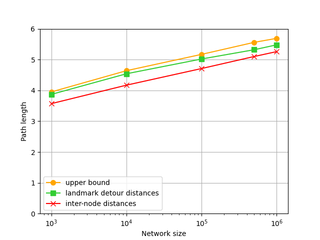
We verify the derived upper bounds on detour distances in BA networks given by (4). Fig. 3 shows a comparison between the derived upper bounds and the simulated detour distances in BA networks. We observe that the theoretical bound is an excellent match with the simulated distances. In addition, the inter-node distances and the theoretical bounds are quite close to the shortest path distances.
Appendix C Ablation study
C.1. Graph Clustering Algorithm
We conducted ablation study such that FluidC is replaced by Louvain algorithm (Blondel et al., 2008) which is widely used for graph clustering and community detection. Table 5 shows that our model performs better with FluidC than with Louvain algorithm in all datasets. The proposed hierarchical clustering using FluidC can control the number of clusters to achieve a good trade-off between complexity and performance. However, Louvain algorithm automatically sets the number of clusters, and the number varied significantly over datasets. Moreover, for COLLAB dataset, Louvain algorithm could not be used due to resource issues. Thus, we conclude that FluidC is the better choice in our framework.
| Dataset | FluidC | Louvain |
|---|---|---|
| COLLAB | 56.24 0.45 | - |
| DDI | 70.97 6.88 | 60.79 8.89 |
| Pubmed | 97.56 0.19 | 95.83 0.23 |
| Cora | 95.40 0.21 | 93.78 0.15 |
| Citeseer | 96.36 0.17 | 94.98 0.12 |
| 99.69 0.00 | 99.30 0.00 |
C.2. Node Centrality
For each cluster, the most “central” node should be selected as the landmark. We have used Degree centrality in this paper; however, there are other types of centrality such as Betweenness and Closeness. Betweenness centrality is a measure of how often a given node is included in the shortest paths between node pairs. Closeness centrality is the reciprocal of the sum-length of shortest paths to the other nodes.
Table 6 shows the experimental results comparing Degree, Betweenness and Closeness centralities. The results show that the performances are similar among the centralities. Thus, all the centralities are effective measures for identifying “important” nodes. Degree centrality, however, was better than the other choices.
More importantly, Betweenness and Closeness centralities require full information on inter-node distances, which incurs high computational overhead. In Table 6, we excluded datasets CITATION2 and COLLAB which are too large graphs to compute Betweenness and Closeness centralities. Scalability is crucial for link prediction methods. Thus we conclude that, from the perspective of scalability and performance, Degree centrality is the best choice.
| Centrality | DDI | PubMed | Cora | Citeseer | |
|---|---|---|---|---|---|
| Degree | 70.03 7.02 | 97.38 0.34 | 94.95 0.18 | 96.15 0.19 | 99.69 0.00 |
| Betweeness | |||||
| Closeness |
Appendix D Actual training time and GPU memory usage
Table 8 and 8 show the comparison and actual training time and GPU memory usage between vanilla GCN with HPLC. Note that HPLC already contains vanilla GCN as a component. Thus, one should attend to the additional resource usage incurred by HPLC in Table 8 and 8. Experiments are conducted with NVIDIA A100 with 40GB memory. We observe that, the additional space and time complexity incurred by HPLC relative to vanilla GCN is quite reasonable, demonstrating the scalability of our framework.
| Dataset | vanilla GCN | HPLC |
|---|---|---|
| CITATION2 | 282856 (ms) | 352670 (ms) |
| COLLAB | 1719 (ms) | 2736 (ms) |
| DDI | 3246 (ms) | 3312 (ms) |
| PubMed | 8859 (ms) | 8961 (ms) |
| Cora | 982 (ms) | 1022 (ms) |
| 1107 (ms) | 1243 (ms) |
| Dataset | vanilla GCN | HPLC |
|---|---|---|
| CITATION2 | 29562 (MB) | 36344 (MB) |
| COLLAB | 4988 (MB) | 7788 (MB) |
| DDI | 2512 (MB) | 2630 (MB) |
| PubMed | 2166 (MB) | 3036 (MB) |
| Cora | 1458 (MB) | 6160 (MB) |
| 2274 (MB) | 2796 (MB) |
Appendix E Dataset
Dataset statistics is shown in Table 9.
Dataset # Nodes # Edges Avg. node deg Density Split ratio Metric Cora 2,708 7,986 2.95 5.9 0.0021% 70/10/20 AUC Citeseer 3,327 7,879 2.36 4.7 0.0014% 70/10/20 AUC PubMed 19,717 64,041 3.25 6.5 0.00033% 70/10/20 AUC Facebook 4,039 88,234 21.85 43.7 0.0108% 70/10/20 AUC DDI 4,267 1,334,889 312.84 500.5 14.67% 80/10/10 Hits@20 CITATION2 2,927,963 30,561,187 10.81 20.7 0.00036% 98/1/1 MRR COLLAB 235,868 1,285,465 5.41 8.2 0.0046% 92/4/4 Hits@50
Appendix F Hyperparameters
F.1. Number of Clusters
Table 10 shows the performance with varying number of clusters. Specifically, where we vary hyperparameter . The results show that performance can be improved by adjusting the number of clusters.
| COLLAB | DDI | PubMed | Cora | Citeseer | ||
|---|---|---|---|---|---|---|
| 55.52 0.51 | 68.27 6.47 | 96.81 0.13 | 94.34 0.16 | 94.70 0.31 | 99.53 0.00 | |
| 55.44 0.80 | 68.95 7.30 | 96.42 0.17 | 94.51 0.18 | 96.43 0.12 | 99.69 0.00 | |
| 56.24 0.45 | 70.97 6.88 | 97.38 0.34 | 94.91 0.11 | 94.85 0.14 | 99.61 0.00 | |
| - | - | 96.89 0.19 | 94.95 0.18 | 96.15 0.19 | 99.63 0.00 | |
| - | - | 97.14 0.17 | 94.34 0.12 | 95.14 0.18 | 99.60 0.00 | |
| - | - | 97.21 0.24 | 94.31 0.19 | 95.87 0.13 | 99.64 0.00 | |
| - | - | 96.76 0.18 | 94.40 0.21 | 95.36 0.17 | 99.65 0.00 |
F.2. Miscellaneous
Miscellaneous hyperparameters are shown in Table 11.
Hyperparameter Value Encoder of all plug-in methods GCN Learning rate 0.001, 0.0005 Hidden dimension 256 Number of GNN layers 2, 3 Number of Decoder layers 2, 3 Negative sampling Uniformly Random sampling Dropout 0.2, 0.5 Negative sample rate 1 Activation function ReLU (GNNs), LeakyReLU () Loss function BCE Loss Use edge weights False (only binary edge weights) The number of landmarks Optimizer Adam (Kingma and Ba, 2015)