Hierarchical Optimal Power Flow with Improved Gradient Evaluation
Abstract
Existing algorithms to solve alternating-current optimal power flow (AC-OPF) often exploit linear approximations to simplify system models and accelerate computations. In this paper, we improve a recent hierarchical OPF algorithm, which rested on primal-dual gradients evaluated in a linearized distribution power flow model. Specifically, we identify a risk of voltage violation arising from the model linearization, and propose a more accurate gradient evaluation method to eliminate that risk. We further develop a hierarchical primal-dual algorithm to solve OPF based on the proposed gradient evaluation method. Numerical results on IEEE networks show that our algorithm can enhance voltage safety with satisfactory computational efficiency.
I Introduction
Optimal power flow (OPF) is a fundamental optimization problem that aims to find a cost-minimizing operating point subject to the physical laws and safety limits of a power network. The power sector is witnessing a rising need for fast and scalable OPF solvers, which can instruct a large network of controllable units (smart appliances, electric vehicles, energy storage devices, etc.) to make timely response to the growing variations of wind and solar generations. Such a need is especially urgent in power distribution networks, where massive renewable energy sources and controllable units are being deployed. However, distribution networks are also where the speed and scalability requirements are most challenging, as the high resistance-to-reactance ratios of distribution lines necessitate nonlinear and nonconvex alternating-current (AC) OPF rather than its simple direct-current approximation.
Numerous efforts have been made to overcome the computational challenges to AC-OPF. Many of them conducted convex relaxations, convex inner approximations, or linearizations of AC power flow; comprehensive reviews were provided in [1, 2]. Meanwhile, distributed OPF algorithms were developed and shown to be more scalable in terms of computation and communication and more robust to single-point failure, compared to their centralized counterparts [3, 4, 5, 6]. To further reduce computational efforts associated with solving AC power flow, some OPF algorithms were implemented by iteratively actuating the power system with intermediate decisions and updating the decisions based on system feedback [7, 8, 9].
From the vast literature, we bring to attention a hierarchical distributed primal-dual gradient algorithm [10] (and its extension to multi-phase networks [11]). It leveraged the radial structure of distribution networks to avoid repetitive computation and communication, and thus significantly accelerated large-scale OPF computations. However, the algorithm in [10] derived approximate gradients from the linearized distribution power flow model in [12, 13]. Such linearization may cause the solver to optimistically estimate nodal voltages to be safe, while they actually already exceed safety limits. The consequent risk of voltage violation will be revealed later in this paper.
To prevent such violation, we develop an improved gradient evaluation method by approximating the partial derivatives of the quadratic terms associated with line currents and power losses. Our analysis shows that with moderate extra computations, the proposed method returns more accurate gradient estimations than [10]. Meanwhile, the proposed method preserves the structure in [10] for gradient evaluation, and thus enables us to develop an improved hierarchical OPF algorithm. Numerical experiments on IEEE 37-node and 123-node networks demonstrate enhanced safety of voltage regulation achieved by the proposed algorithm with a moderate increase in computation time, compared to the previous method based on the linearized model.
The rest of this paper is organized as follows. Section II introduces the distribution network model, the OPF problem, and a primal-dual algorithm to solve it. Section III motivates and elaborates the improved gradient evaluation method. Section IV presents the hierarchical OPF algorithm based on the improved gradient evaluation. Section V reports the numerical experiments. Section VI concludes this paper.
II Modeling and Preliminary Algorithm
II-A Power network model and OPF problem
We model a single-phase equivalent power distribution network as a directed tree graph , where , with indexing the root node (the substation, also known as the slack bus), and indexing other nodes. The set collects the ordered pairs of nodes representing the lines in the network. We define the directions of lines as pointing away from the root, e.g., in line , node is closer to the root than node . Let and denote the net active and reactive power injections (i.e., power supply minus consumption) and denote the squared voltage magnitude at each node . Let denote the squared current magnitude, denote the series impedance, and and denote the sending-end active and reactive power on each line .
We adopt the distribution power flow model [12, 13]:
| (1a) | ||||
| (1b) | ||||
| (1c) | ||||
| (1d) | ||||
Assume the power injections to be controllable within a given operating region:
| (2) |
Define vectors , , . Following [8], we express the voltage vector as a function of power injections, i.e., , implicitly defined by (1). Consider the following OPF problem:
| (3a) | ||||
| s.t. | (3b) | |||
| (3c) | ||||
where is a strongly convex cost function for the control of power injections at node , inequality (3b) is element-wise, given constant squared voltage limits and .
II-B Primal-dual gradient algorithm
Let and be the dual variables associated with (3b) to penalize the violation of voltage lower and upper bounds, respectively. To design a convergent primal-dual algorithm, we consider the regularized Lagrangian of (3):
| (4) |
where and is a constant factor for the regularization term. Function (II-B) is strongly convex in primal variables and strongly concave in dual variables . The saddle point of (II-B) serves as an approximate solution to (3), with a bounded error that is linear in [10, 14]. The following primal-dual gradient algorithm has been commonly used to iteratively approach such a saddle point:
| (5a) | |||
| (5b) | |||
| (5c) | |||
where collects the controllable power injections; is the objective (3a); both denote the voltage profile under power injections at time step . Note that does not have to be calculated by (1) or any other mathematical model of power flow; instead, it can be measured from the power network after actuating the network with the intermediate decisions during the process (5). This feedback-based implementation has been widely adopted to compensate for likely modeling errors [7, 8, 9, 11]. The subscripts and represent the projections onto and the nonnegative orthant, respectively. Without loss of generality, we use constant step sizes to update the primal and dual variables, respectively.
The gradient in (5a) can be easily computed, and the voltage in (5b)–(5c) can be conveniently measured, both locally at each node . Therefore, the remaining key challenge is to compute the gradient that potentially couples all the nodes in the power network. This will be addressed in the next section.
III Improved Gradient Evaluation
III-A Prior work and motivation for improvement
In power flow equations (1), the nonlinear and implicit dependence of voltage on power injections makes it difficult to quickly and precisely compute the gradient . Reference [8] proposed a backward-forward sweep method for gradient calculation, which is computationally inefficient in large networks. In contrast, prior work [10] considered the linearized power flow model in [12, 13]:
| (6a) | ||||
| (6b) | ||||
| (6c) | ||||
which yields the following approximation of :
| (7a) | |||
| (7b) | |||
where denotes the common part of the unique paths from nodes and back to the root node.
We illustrate the error of linear model (6) by introducing the following Lemma.
Lemma 1
Let and denote the active and reactive power loss downstream of node . The voltage error induced by (6) for all is:
| (8) |
where the expressions of and are:
Proof:
See Appendix.
Lemma 1 reveals that the voltage computed with the linear model (6) is higher than that under the accurate nonlinear model (1). Such errors would accumulate as we trace the nodes further away from the root. Therefore, under the power injections solved by (5) with the linear model (6) and the approximate gradient (7), even though the model optimistically estimates the voltages to be safe, the actual voltages may already drop below their lower bounds. The need to prevent such voltage violation motivates us to develop an improved gradient evaluation method, as elaborated below.
III-B Improved gradient evaluation
Consider an arbitrary node , and . We take the partial derivatives of the variables in the nonlinear power flow model (1):
| (9a) | ||||
| (9b) | ||||
| (9c) | ||||
| (9d) | ||||
The exact partial derivatives are hard to solve from (9) due to their complex interdependence. To facilitate computation, we first simplify (9d) by replacing the partial derivatives with their approximations under the linear model (6):
| (10) |
We recall the following results from [8] for all the nodes and lines :
| (11a) | ||||||
| (11b) | ||||||
where is an indicator that equals 1 if node lies on the unique path from node to the root, and 0 otherwise. By (11) and (7), we can calculate in (10) as follows:
| (12a) | ||||
| (12b) | ||||
The results in (7), (11), (12) can replace the partial derivatives on the right-hand side (RHS) of (9c) to obtain an improved gradient evaluation as:
| (13a) | |||
| (13b) | |||
where node is the unique parent of node in the directed tree network. By (7a), there is , which converts the result in (13a) into:
| (14) |
The first term on the RHS of (14) is the same as (7a) derived from the linear model (6), while the second and third terms compensate for the effects of the quadratic terms that were neglected from (6). The improved partial derivatives (13b) with respect to reactive power injections have the same structure as (13a), and thus we will not repeat.
IV Hierarchical OPF Algorithm
Based on the primal-dual framework (5) and the improved gradient evaluation (13), we design a scalable hierarchical algorithm to solve the OPF problem (3). The proposed algorithm utilizes the subtree structure of radial distribution networks discovered in [11, 10], while achieving more accurate and safer voltage regulation.
The distribution tree network is composed of subtrees indexed by and a set of nodes that are not clustered into any subtree. Let denote the root node of subtree , which is the node in that is nearest to the root node of the whole network. Given a distribution network, the division of subtrees and unclustered nodes may not be unique, but we assume it always satisfies the following conditions.
Assumption 1
The subtrees are non-overlapping, i.e., for any , .
Assumption 2
For any subtree root node , or any unclustered node , its path to the network root node only goes through a subset of nodes in , but not any node in another subtree.
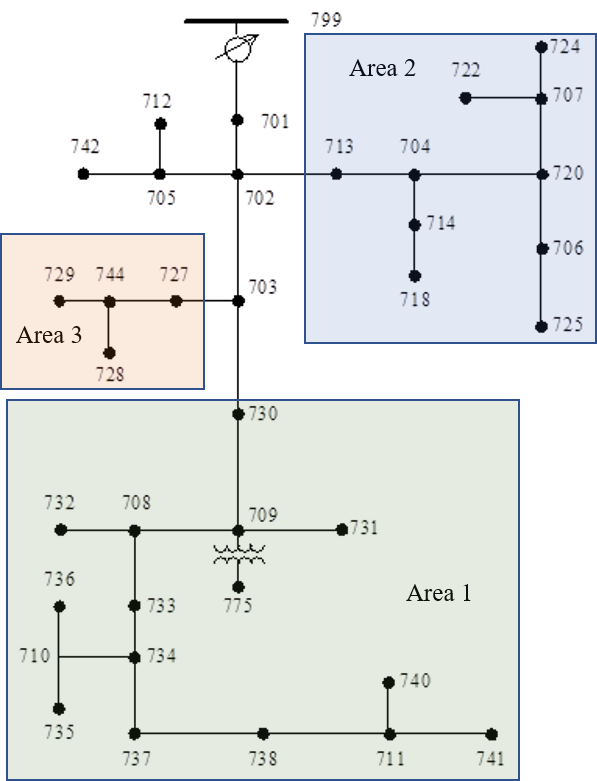
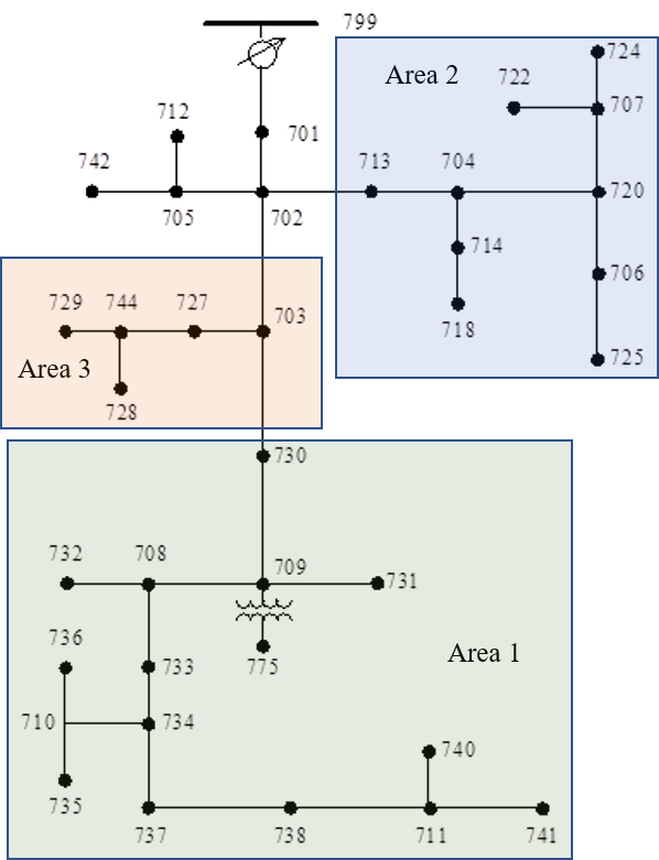
The left subfigure of Figure 1 shows a clustering of the IEEE 37-node network that satisfies Assumption 2, while the one in the right subfigure does not.
The distribution system operator plays a role of central controller (CC). It is sufficient for the CC to know the structure and parameters of the backbone network, which only connects the unclustered nodes and the subtree root nodes . The CC also maintains two-way communications to receive/send/relay information from/to/between the backbone network nodes. Each subtree network is known to and managed by the -th regional controller (RC ), which communicates with the nodes in subtree , the parent node of the subtree root , and the CC.
With the settings above, we now explain the hierarchical structure underlying the vector in (5a). Without loss of generality, we only consider the element of this vector corresponding to for a particular node , which can be discussed in two cases below. The element corresponding to can be calculated in the same manner.
Case 1: If is in a subtree , we have:
| (15) |
The first term on the RHS of (15) sums over nodes in the same subtree as node . It can be calculated using (13a) by RC , and then sent to node which requires this information to compute (15) and carry out (5a). In particular, the calculation of requires RC to receive parameters , and measurements , , from line that connects node to its parent node .
The second term on the RHS of (15) sums over nodes in all the subtrees except subtree that hosts node . By Assumption 2, there must be , which simplifies (13a) and leads to:
| (16) |
In (16), the sum over can be calculated by RC . The CC receives such sums from all the RCs , adds them up after weighting by , and sends the result to RC . Upon receiving this result, RC broadcasts it to all the nodes in subtree , including node which requires this information to compute (15) and carry out (5a).
The third term on the RHS of (15) sums over all the unclustered nodes . It can be calculated using (13a) by the CC and then relayed by RC to node . In particular, and are known to the CC for the calculation of (13a).
Case 2: If is an unclustered node, we have:
| (17) | |||||
The first term on the RHS of (17) sums over nodes in all the subtrees . By Assumption 2, there must be , which simplifies (13a) and leads to:
| (18) |
In (18), the sum over can be calculated by RC . The CC receives such sums from all the RCs , adds them up after weighting by , and sends the result to node for subsequent computations of (17) and (5a).
The second term on the RHS of (17) sums over all the unclustered nodes . It can be calculated using (13a) by the CC and then sent to node . In particular, and are known to the CC for the calculation of (13a), since node , its parent node , and node are all in the backbone network.
To summarize, the computation of the key term in (5a) can be performed through the coordination of the CC and the RCs in a hierarchical manner. This inspires our design of Algorithm 1 to solve the OPF problem (3). Compared to the conventional centralized primal-dual gradient method, the hierarchical Algorithm 1 can reduce computational complexity as analyzed in [11]. Due to space limitation, the convergence proof of Algorithm 1 is deferred to the journal version of this work.
V Numerical Experiments
We conduct numerical experiments to demonstrate our improvement over the previous method [10] based on the linearized power flow model (6).
V-A Experiment setup
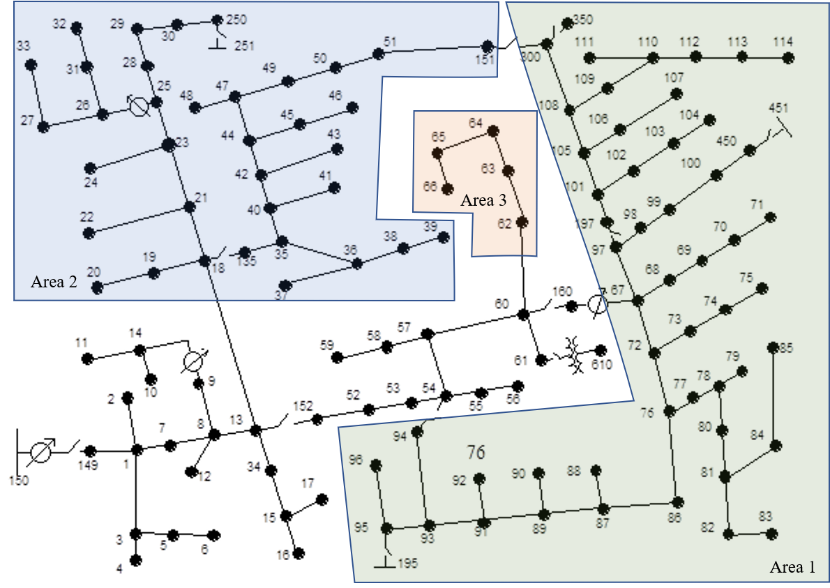
We consider the single-phase equivalent models of the IEEE 37-node and 123-node test networks. They are clustered into subtrees as shown by Figure 1 (left panel) and Figure 2, respectively.
For the ease of illustration, we make the following modifications to the original network models on the IEEE PES website (https://cmte.ieee.org/pes-testfeeders/resources/):
-
1.
We model each multi-phase line as a single-phase line with the average impedance of multiple phases. We also convert the multi-phase wye- and delta-connected loads into single-phase loads by taking their average over multiple phases.
-
2.
We multiply the original load data of the 37-node network by six, and those of the 123-node network by two, to create scenarios with serious voltage issues.
-
3.
All the loads are treated as constant-power loads. Detailed models of capacitors, regulators, and breakers are not simulated.
For each network, let denote the set of nodes that host nonzero loads. We denote the negative net power injections from the IEEE load data by for all load nodes , and treat them as the nominal injections or the most preferred injections. The feasible power injection regions in (2) are defined as . The OPF objective function in (3a) is defined as for all , which aims to minimize the disutility caused by the deviation from the nominal loads.
For each network, the voltage magnitude of the root (slack) node is fixed at per unit (p.u.). The lower and upper limits for safe voltage are set at p.u. and p.u., respectively. The step sizes for primal and dual variable updates are empirically chosen as and , respectively.
For each given power injection , an OpenDSS power flow simulation is performed to obtain the corresponding voltage and the associated line-flow quantities , which are treated as the feedback signals measured from the power network. The Python 3.7 programs for OPF algorithms and the OpenDSS simulations are run on a laptop equipped with Intel Core i7-9750H CPU @ 2.6 GHz, 16 GB RAM, and Windows 10 Professional OS.
V-B Numerical results
Due to space limitation, we only show the simulation results in the 123-node network model. The results in the 37-node network are similar.
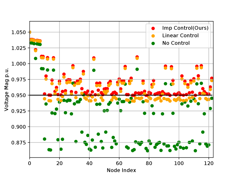
Voltage safety: The voltage magnitudes at different nodes of the 123-node network are plotted in Figure 3, for three cases. The first case, referred to as “no control”, just takes the nominal power injections from the IEEE data, which causes severe violation of the voltage lower bound. The second case, referred to as “linear control”, applies the primal-dual gradient algorithm in [10] based on the linearized power flow model (6) to determine power injections, which enhances the overall voltage level but still leaves most nodes below the voltage lower bound. The third case, referred to as “improved control (ours)”, solves the OPF with the proposed Algorithm 1 based on our improved gradient evaluation method, which effectively lifts all the voltages above the lower bound. This result verifies our analysis in Section III that the improved gradient evaluation can prevent voltage violation caused by the linear model that optimistically estimates the voltages to be safe.
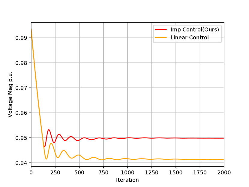
Computational efficiency: Figure 4 shows the change of voltage at a node of the 123-node network (similar trends are displayed for the voltages at other nodes). This result verifies again that the voltage converges to a safe level under the proposed Algorithm 1, compared to the previous algorithm [10] that leads to a violation of voltage lower bound. Moreover, Algorithm 1 converges in fewer iterations. Indeed, Algorithm 1 spends 205 seconds to complete 2,000 iterations, compared to the previous algorithm in [10] which spends 166 seconds. This would be an acceptable increase, considering the improved voltage safety achieved by Algorithm 1.
VI Conclusion
We proposed a hierarchical OPF algorithm based on a new gradient evaluation method that is more accurate than previous methods based on the linearized power flow model. The proposed method can prevent the previous voltage violation with moderate extra computations, as verified by numerical results on IEEE networks.
In future work, we will provide formal convergence proof and complexity analysis of the proposed algorithm. We will also extend the proposed algorithm to multi-phase networks, as what was done from [10] to [11].
[Proof of Lemma 1]

Proof: Take the difference between the linear model (6) and the actual nonlinear model (1):
| (20a) | ||||
| (20b) | ||||
| (20c) | ||||
Substitute (20b)–(20c) into (20a), which yields:
| (21) |
We further calculate the active and reactive power loss terms and on the RHS of (VI). Following the tree structure of the network (i.e., a tree graph shown by Figure 5), we recursively calculate (20b)–(20c) until reaching leaves:
| (22a) | ||||
| (22b) | ||||
| (22c) | ||||
| (22d) | ||||
We substitute the above equations layer-by-layer, i.e., (22c), , into (22a) for active power and (22d), , into (22b) for reactive power. This gives the expression of the active and reactive power loss terms as:
| (23a) | |||
| (23b) | |||
| (23c) | |||
| (23d) | |||
We define and as the additive inverse of RHS of (23b) and (23d), respectively. In fact, and sum the active and reactive power loss of the lines downstream of node . We have more compact expressions for and :
where denotes the set of lines downstream of node . From the tree structure, we have:
| (25a) | |||
| (25b) | |||
The expressions of (25) imply that a backward sweep from the leaves to the root node in a power distribution network will give all the results of . With , the voltage error (VI) becomes:
| (26) |
Equation (26) implies that the voltage error is accumulated from the root to the leaves. A forward sweep from the root to leaves will return voltage error for all nodes as:
This completes the proof of Lemma 1.
References
- [1] S. H. Low, “Convex relaxation of optimal power flow—Part I: Formulations and equivalence,” IEEE Transactions on Control of Network Systems, vol. 1, no. 1, pp. 15–27, 2014.
- [2] D. K. Molzahn and I. A. Hiskens, “A survey of relaxations and approximations of the power flow equations,” Foundations and Trends in Electric Energy Systems, pp. 1–221, 2019.
- [3] E. Dall’Anese, H. Zhu, and G. B. Giannakis, “Distributed optimal power flow for smart microgrids,” IEEE Transactions on Smart Grid, vol. 4, no. 3, pp. 1464–1475, 2013.
- [4] T. Erseghe, “Distributed optimal power flow using ADMM,” IEEE Transactions on Power Systems, vol. 29, no. 5, pp. 2370–2380, 2014.
- [5] B. Zhang, A. Y. Lam, A. D. Domínguez-García, and D. Tse, “An optimal and distributed method for voltage regulation in power distribution systems,” IEEE Transactions on Power Systems, vol. 30, no. 4, pp. 1714–1726, 2015.
- [6] Q. Peng and S. H. Low, “Distributed optimal power flow algorithm for radial networks, I: Balanced single phase case,” IEEE Transactions on Smart Grid, vol. 9, no. 1, pp. 111–121, 2018.
- [7] S. Bolognani, R. Carli, G. Cavraro, and S. Zampieri, “Distributed reactive power feedback control for voltage regulation and loss minimization,” IEEE Transactions on Automatic Control, vol. 60, no. 4, pp. 966–981, 2015.
- [8] L. Gan and S. H. Low, “An online gradient algorithm for optimal power flow on radial networks,” IEEE Journal on Selected Areas in Communications, vol. 34, no. 3, pp. 625–638, 2016.
- [9] A. Bernstein and E. Dall’Anese, “Real-time feedback-based optimization of distribution grids: A unified approach,” IEEE Transactions on Control of Network Systems, vol. 6, no. 3, pp. 1197–1209, 2019.
- [10] X. Zhou, Z. Liu, W. Wang, C. Zhao, F. Ding, and L. Chen, “Hierarchical distributed voltage regulation in networked autonomous grids,” in American Control Conference, pp. 5563–5569, 2019.
- [11] X. Zhou, Z. Liu, C. Zhao, and L. Chen, “Accelerated voltage regulation in multi-phase distribution networks based on hierarchical distributed algorithm,” IEEE Transactions on Power Systems, vol. 35, no. 3, pp. 2047–2058, 2019.
- [12] M. Baran and F. F. Wu, “Optimal sizing of capacitors placed on a radial distribution system,” IEEE Transactions on Power Delivery, vol. 4, no. 1, pp. 735–743, 1989.
- [13] M. Farivar and S. H. Low, “Branch flow model: Relaxations and convexification—part I,” IEEE Transactions on Power Systems, vol. 28, no. 3, pp. 2554–2564, 2013.
- [14] J. Koshal, A. Nedić, and U. V. Shanbhag, “Multiuser optimization: Distributed algorithms and error analysis,” SIAM Journal on Optimization, vol. 21, no. 3, pp. 1046–1081, 2011.