Hierarchical Low-Rank Approximation of Regularized Wasserstein Distance
Abstract
Sinkhorn divergence is a measure of dissimilarity between two probability measures. It is obtained through adding an entropic regularization term to Kantorovich’s optimal transport problem and can hence be viewed as an entropically regularized Wasserstein distance. Given two discrete probability vectors in the -simplex and supported on two bounded subsets of , we present a fast method for computing Sinkhorn divergence when the cost matrix can be decomposed into a -term sum of asymptotically smooth Kronecker product factors. The method combines Sinkhorn’s matrix scaling iteration with a low-rank hierarchical representation of the scaling matrices to achieve a near-linear complexity . This provides a fast and easy-to-implement algorithm for computing Sinkhorn divergence, enabling its applicability to large-scale optimization problems, where the computation of classical Wasserstein metric is not feasible. We present a numerical example related to signal processing to demonstrate the applicability of quadratic Sinkhorn divergence in comparison with quadratic Wasserstein distance and to verify the accuracy and efficiency of the proposed method.
keywords optimal transport, Wasserstein metric, Sinkhorn divergence, hierarchical matrices
1 Introduction
Wasserstein distance is a measure of dissimilarity between two probability measures, arising from optimal transport; see e.g. [16, 17]. Due to its desirable convexity and convergence features, Wasserstein distance is considered as an important measure of dissimilarity in many applications, ranging from computer vision and machine learning to Seismic and Bayesian inversion; see e.g. [13, 5, 18, 11]. The application of Wasserstein metric may however be limited to cases where the probability measures are supported on low-dimensional spaces, because its numerical computation can quickly become prohibitive as the dimension increases; see e.g. [13].
Sinkhorn divergence [3] is another measure of dissimilarity related to Wasserstein distance. It is obtained through adding an entropic regularization term to the Kantorovich formulation of optimal transport problem. It can hence be viewed as a regularized Wasserstein distance with desirable convexity and regularity properties. A main advantage of Sinkhorn divergence over Wasserstein distance lies in its computability by an iterative algorithm known as Sinkhorn’s matrix scaling algorithm [14], where each iteration involves two matrix-vector products. Consequently, Sinkhorn divergence may serve as a feasible alternative to classical Waaserstein distance, particularly when probability measures are supported on multi-dimensional spaces in with .
Given a cost function and two -dimensional discrete probability vectors supported on two measurable subsets of the Euclidean space , it is known that Sinkhorn’s algorithm can compute an -approximation of the original Kantorovich optimal transport problem within iterations [4]. If the matrix-vector products needed in each iteration of the algorithm are performed with cost , the overall complexity of the algorithm for computing Sinkhorn divergence will be . While theoretically attainable, this quadratic cost may still prohibit the application of Sinkhorn divergence to large-scale optimization problems that require many evaluations of Sinkhorn-driven loss functions.
In the present work, we will develop a hierarchical low-rank strategy that significantly reduces the quadratic cost of Sinkhorn’s algorithm to a near-linear complexity . We consider a class of cost matrices in optimal transport that can be decomposed into a -term sum of Kronecker product factors, where each term is asymptotically smooth. Importantly, such class of cost matrices induce a wide range of optimal transport distances, including the quadratic Wasserstein metric and its corresponding Sinkhorn divergence. We then propose a strategy that takes two steps to reduce the complexity of each Sinkhorn iteration from to . We first exploit the block structure of Kronecker product matrices and turn the original (and possibly high-dimensional) matrix-vector product problems into several smaller one-dimensional problems. The smaller problems will then be computed by the hierarchical matrix technique [7], thanks to their asymptotic smoothness, with a near-linear complexity. We further present a thorough error-complexity analysis of the proposed hierarchical low-rank Sinkhorn’s algorithm.
The rest of the paper is organized as follows. In Section 2 we review the basics of Wasserstein and Sinkhorn dissimilarity measures in optimal transport and include a short discussion of the original Sinkhorn’s algorithm. We then present and analyze the proposed hierarchical low-rank Sinkhorn’s algorithm for computing Sinkhorn divergence in Section 3. In Section 4 we present a numerical example related to a signal processing optimization problem to demonstrate the applicability, accuracy, and efficiency of the proposed method. Finally, in Section 5 we summarize conclusions and outline future works.
2 Optimal transport dissimilarity measures
In this section, we present the basics of the Kantorovich formulation of optimal transport and review two related dissimilarity measures; the Wasserstein distance and the Sinkhorn divergence. We focus on probability vectors, rather than working with more general probability measures.
2.1 Kantorovich’s optimal transport problem and Wasserstein distance
Let and be two measurable subsets of the Euclidean space , with . Let further and be two -dimensional probability vectors, i.e. two vectors in the probability simplex , defined on and , respectively. Here, is the -dimensional vector of ones. The two probability vectors and are assumed to be given at two sets of discrete points and in , respectively. Figure 1 shows a schematic representation of probability vectors in and dimensions.


We denote by the transport polytope of and , i.e. the set of all nonnegative matrices with row and column sums equal to and , respectively, that is,
Each matrix in the transport polytope is a transport (or coupling) matrix that encodes a transport plan, that is, each element of describes the amount of mass to be transported from a source point to a traget point , with . The two constraints and are necessary for a transport plan to be admissible; all the mass taken from a point , i.e. , must be equal to the mass at point , i.e. , and all the mass transported to a point , i.e. , must be equal to the mass at point , i.e. . We say that and are the marginals of .
Let further be a non-negative cost function defined on . For any pair of points , the value represents the cost of transporting one unit of mass from a source point to a target point . Correspondingly, we consider the cost matrix
The optimal transport problem can now be formulated as follows. We first note that for any given transport plan , the total transport cost associated with is given by the Frobenius inner product . Kantorovich’s optimal transport problem then aims at minimizing the total transport cost over all admissible transport plans. It reads
| (1) |
where is the optimal total cost of transporting onto .
In some applications the main goal of solving Kantorovich’s optimal transport problem (1) is to find the optimal transport plan, i.e. the transport matrix that minimizes the total cost. In some other applications the goal is to directly find the optimal cost without the need to explicitly form the optimal transport matrix. An example of the latter application appears in the construction of loss functions in optimization problems, where loss functions are built based on metrics induced by the optimal cost . An important type of such metrics is Wasserstein metric.
For the optimal cost in (1) to induce a metric, we need the cost matrix to be a metric matrix belonging to the cone of distance matrices [17], i.e. we need , where
Throughout this paper, we always assume that the cost matrix is a metric matrix: . An important class of metric matrices is driven by cost functions of the form , where , and is a distance function (or metric). In this case the cost matrix reads
| (2) |
Intuitively, this choice implies that the cost of transporting one unit of mass from a source point to a target point corresponds to the distance between the two points. The optimal cost in (1) corresponding to the cost matrix (2) induces a metric known as the Wasserstein distance of order [16, 17],
| (3) |
Due to its desirable convexity and convergence features, Wasserstein distance is considered as an important measure of dissimilarity in many applications, ranging from computer vision and machine learning to Seismic and Bayesian inversion; see e.g. [13, 5, 18, 11]. Unfortunately, the numerical computation of Wasserstein metric is in general infeasible in high dimensions and is mainly limited to low dimensions; see e.g. [13]. For instance, in the case , the quadratic Wasserstein distance between two continuous probability density functions and is given by [2]
where is the optimal map. In one dimension, i.e. when , the optimal map is given by , where and are the cumulative distribution functions corresponding to and , respectively. The discrete metric between the corresponding probability vectors and can then be efficiently approximated by a quadrature rule,
where may be computed by interpolation and an efficient search algorithm, such as binary search. The overall cost of computing the discrete metric in one dimension will then be . In multiple dimensions, i.e. when with , however, the computation of the optimal map , and hence the metric, may be either expensive or infeasible. The map is indeed given by the gradient of a convex function that is the solution to a constrained nonlinear Monge-Ampère equation. We refer to [5] for more discussion on the finite difference approximation of the Monge-Ampère equation in two dimensions.
2.2 Entropy regularized optimal transport and Sinkhorn divergence
One approach to computing Kantorovich’s optimal transport problem (1) is to regularize the original problem and seek approximate solutions to the regularized problem. One possibility is to add an entropic penalty term to the total transport cost and arrive at the regularized problem
| (4) |
where is a regularization parameter, and is the discrete entropy of transport matrix,
| (5) |
The regularized problem (4)-(5) with has a unique solution, say [3]. Indeed, the existence and uniqueness follows from the boundedness of and the strict convexity of the negative entropy. On the one hand, as increases, the unique solution converges to the solution with maximum entropy within the set of all optimal solutions of the original Kantorovich’s problem; see Proposition 4.1 in [13],
In particular, we have . On the other hand, as decreases, the unique solution converges to the transport matrix with maximum entropy between the two marginals and , i.e. the outer product of and ; see Proposition 4.1 in [13],
It is to be noted that in this latter case, as , the optimal solution becomes less and less sparse (or smoother), i.e. with more and more entries larger than a prescribed small threshold.
With being the optimal solution to the regularized problem (4)-(5) corresponding to the cost matrix (2), the Sinkhorn divergence of order between and is defined as
| (6) |
Sinkhorn divergence (6) has several important properties. First, it satisfies all axioms for a metric with the exception of identity of indiscernibles (or the coincidence axiom), that is, it satisfies non-negativity, symmetry, and triangle inequality axioms [3]. Second, it is convex and smooth with respect to the input probability vectors and can be differentiated using automatic differentiation [13]. Third, as discussed below, it can be computed by a simple alternating minimization algorithm, known as Sinkhorn’s algorithm, where each iteration involves two matrix-vector products. Consequently, Sinkhorn divergence may serve as a feasible alternative to classical Waaserstein distance, particularly when probability measures are supported on multi-dimensional metric spaces.
Proof.
Sinkhorn’s algorithm. Adding an entropic penalty term to the optimal transport problem enforces a simple structure on the regularized optimal transport matrix . Introducing two dual variables and for the two marginal constraints and in , the Lagrangian of (4)-(5) reads
Setting , we obtain
| (8) |
We can also write (8) in matrix factorization form,
| (9) |
A direct consequence of the form (8), or equivalently (9), is that is non-negative, i.e. . Moreover, it implies that the computation of amounts to computing two non-negative vectors , known as scaling vectors. These two vectors can be obtained from the two marginal constraints,
| (10) |
Noting that and , we arrive at the following nonlinear equations for ,
| (11) |
where denotes the Hadamard (or entrywise) product. Problem (10), or equivalently (11), is known as the non-negative matrix scaling problem (see e.g. [9, 12]) and can be solved by an iterative method known as Sinkhorn’s algorithm [14],
| (12) |
Here, denotes the Hadamard (or entrywise) division. We note that in practice we will need to use a stopping criterion. One such criterion may be defined by monitoring the difference between the true marginals and the marginals of the most updated solutions. Precisely, given a small tolerance , we continue Sinkhorn iterations until we obtain
| (13) |
After computing the scaling vectors , the -Sinkhorn divergence can be computed as
| (14) |
We refer to Remark 4.5 of [13] for a historic perspective of the matrix scaling problem (11) and the iterative algorithm (12).
Convergence and complexity. Suppose that our goal is to compute an -approximation of the optimal transport plan,
where is a positive small tolerance. This can be achieved within Sinkhorn iterations if we set [4]. See also [1] for a less sharp bound on the number of iterations. The bounds presented in [4, 1] suggest that the number of iterations depends weakly on . The main computational bottleneck of Sinkhorn’s algorithm is however the two vector-matrix multiplications against kernels and needed in each iteration with complexity if implemented naively. Overall, Sinkhorn’s algorithm can compute an -approximate solution of the unregularized OT problem in operations. We also refer to Section 4.3 in [13] for a few strategies that may improve this complexity. In particular, the authors in [15] exploited possible separability of cost metrics (closely related to assumption A1 in Section 3.1 of the present work) to reduce the quadratic complexity to ; see also Remark 4.17 in [13]. It is to be noted that although this improved cost is no longer quadratic (except when ), the resulting algorithm will still be a polynomial time algorithm whose complexity includes a term with . Our goal here is to exploit other possible structures in the kernels and further reduce the cost to a log-linear cost, thereby delivering an algorithm that runs faster than any polynomial time algorithm.
Remark 1.
(Selection of ) On the one hand, the regularization parameter needs to be large enough for the regularized OT problem to be close to the original OT problem. This is indeed reflected in the choice that enables achieving an -approximation of the optimal transport plan: the smaller the tolerance , the larger . On the other hands, the convergence of Sinkhorn’s algorithm deteriorates as ; see e.g. [6, 10]. Moreover, as , more and more entries of the kernel (and hence entries of and ) may become “essentially” zero. In this case, Sinkhorn’s algorithm may become numerically unstable due to division by zero. The selection of the regularization parameter should therefore be based on a trade-off between accuracy, computational cost, and robustness.
3 A fast algorithm for computing Sinkhorn divergence
We consider an important class of cost matrices for which the complexity of each Sinkhorn iteration can be significantly reduced from to . Precisely, we consider cost matrices that can be decomposed into a -term sum of Kronecker product factors, where each term is asymptotically smooth; see Section 3.1. The new Sinkhorn’s algoritm after iterations will then have a near-linear complexity ; see Section 3.2 and Section 3.3. Importantly, such class of cost matrices induce a wide range of optimal transport distances, including the quadratic Wasserstein metric and its corresponding Sinkhorn divergence.
3.1 Main assumptions
To make the assumptions precise, we first introduce a special Kronecker sum of matrices.
Definition 1.
The “all-ones Kronecker sum” of two matrices and , denoted by , is defined as
where is the all-ones matrix of size , and denotes the standard Kronecker product.
It is to be noted that the all-ones Kronecker sum is different from the common Kronecker sum of two matrices in which identity matrices and replace all-ones matrices and . This new operation facilitates working with elementwise matrix operations. We also note that the two-term sum in Definition 1 can be recursively extended to define all-ones Kronecker sums with arbitrary number of terms, thanks to the following associative property inherited from matrix algebra,
We next consider kernel matrices generated by kernel functions with a special type of regularity, known as “asymptotic smoothness” [7].
Definition 2.
A kernel function on the real line is said to be “asymptotically smooth” if there exist constants such that for some the following holds,
| (15) |
A kernel matrix , generated by an asymptotically smooth kernel function , is called an asymptotically smooth kernel matrix.
We now make the following two assumptions.
-
A1.
The cost matrix can be decomposed into a -term all-ones Kronecker sum
(16) where each matrix is generated by a metric on the real line.
-
A2.
The kernel matices and , with , generated by the kernels and , where , are asymptotically smooth.
It is to be noted that by assumption A2 all kernels and , with , satisfy similar estimates of form (15) with possibly different sets of constants .
cost functions. An important class of cost functions for which assumptions A1-A2 hold includes the cost functions, given by
| (17) |
Here, denotes the -norm in , with . Importantly, such cost functions take the form of (2) with , for which -Wasserstein metric and -Sinkhorn divergence are well defined. In particular, the case corresponds to the quadratic Wasserstein metric.
We will first show that assumption A1 holds for cost functions. Let the two sets of discrete points and , at which the two probability vectors are defined, be given on two regular grids in . We note that if the original probability vectors are given on irregular grids, we may find their values on regular grids by interpolation with a cost that would not change the near-linearity of our overall target cost. Set . Then, to each pair of indices and of the cost matrix , we can assign a pair of -tuples and in the Cartesian product of finite sets , where . Consequently, the additive representation of in (17) will imply (16).
It is also easy to see that assumption A2 holds for cost functions, with corresponding kernels,
Indeed, these kernels are asymptotically smooth due to the exponential decay of as increases. For instance, in the particular case when , the estimate (15) holds for both and with , , , and . To show this, we note that
where is the Hermite polynomial of degree , satisfying the following inequality [8],
Setting , and noting that for , we obtain
Hence we arrive at
Similarly, we can show that the same estimate holds for .
3.2 Hierarchical low-rank approximation of Sinkhorn iterations
As noted in Section 2.2, the main computational bottleneck of Sinkhorn’s algorithm is the matrix-vector multiplications by kernels and in each iteration (12) and by kernel in (14). We present a strategy that reduces the complexity of each Sinkhorn iteration to , enabling Sinkhorn’s algorithm to achieve a near-linear overall complexity . The proposed strategy takes two steps, following two observations made based on assumptions A1 and A2.
3.2.1 Step 1: decomposition into 1D problems
A direct consequence of assumption A1 is that both kernel matrices and have separable multiplicative structures.
Proposition 2.
Under assumption A1 on the cost matrix , the matrices and will have Kronecker product structures,
| (18) |
| (19) |
Proof.
Exploiting the block structure of the Kronecker product matrices and , one can compute the matrix-vector products , , and without explicitly forming and . This can be achieved using the vector operator that transforms a matrix into a vector by stacking its columns beneath one another. We denote by the vectorization of matrix formed by stacking its columns into a single column vector .
Proposition 3.
Let , where and . Then, the matrix-vector multiplication , where , amounts to matrix-vector multiplications for different vectors , with .
Proof.
The case is trivial, noting that . Consider the case . Then we have , with , , and . Let be the matrix whose vectorization is the vector , i.e. . Then, we have
Hence, computing amounts to computing . This can be done in two steps. We first compute ,
where is the -th row of matrix in the form of a column vector. For this we need to perform matrix-vector multiplies , with . We then compute ,
where is the -th column of matrix . We therefore need to perform matrix-vector multiplies , with . Overall, we need matrix-vector multiplies for different vectors , and matrix-vector multiplies for different vectors , as desired. This can be recursively extended to any dimension . Setting , we can write
| (20) |
This can again be done in two steps. We first compute , where with ,
where is the -th row of matrix in the form of a column vector. To compute we need to perform matrix-vector multiplies , with We then compute ,
where is the -th column of matrix . We therefore need to perform matrix-vector multiplies , with . Noting that each multiply is of the same form as the multiply (20) but in dimensions, the proposition follows easily by induction. ∎
Reduction in complexity due to step 1. Proposition 2 and Proposition 3 imply
| (21) |
Indeed, the original -dimensional problems and turn into several smaller one-dimensional problems of either or form. This already amounts to a significant gain in efficiency. For instance, if we compute each of these smaller problems by performing floating-point arithmetic operations, then the complexity of will become
And in the particular case when , we will have
It is to be noted that this improvement in the efficiency (for ) was also achieved in [15]. Although this improved cost is no longer quadratic (except in 1D problems when ), the resulting algorithm will still be a polynomial time algorithm whose complexity includes a term with . For instance for 2D and 3D problems (considered in [15]), the overall complexity of Sinkhorn’s algorithm after iterations would be and , respectively. In what follows, we will further apply the technique of hierarchical matrices to the smaller one-dimensional problems, thereby delivering an algorithm that achieves log-linear complexity and hence runs faster than any polynomial time algorithm.
3.2.2 Step 2: approximation of 1D problems by hierarchical matrices
We will next present a fast method for computing the smaller 1D problems and obtained in step 1. We will show that, thanks to assumption A2, the hierarchical matrix technique [7] can be employed to compute each one-dimensional problem with a near-linear complexity .
Since by assumption A2 the kernels and that generate and , with , are all asymptotically smooth and satisfy similar estimates of form (15), the numerical treatment and complexity of all one-dimensional problems will be the same. Hence, in what follows, we will drop the dependence on and consider a general one-dimensional problem , where is a kernel matrix generated by a one-dimensional kernel satisfying (15). Precisely, let be an index set with cardinality . Consider the kernel matrix
uniquely determined by two sets of discrete points and and an asymptotically smooth kernel , with , satisfying (15). Let denote a matrix block of the square kernel matrix , characterized by two index sets and . We define the diameter of and the distance between and by
The two sets of discrete points and the position of the matrix block is illustrated in Figure 2. Note that when the cardinality of the index sets and are equal (), the matrix block will be a square matrix.

The hierarchical matrix technique for computing consists if three parts (see details below):
-
I.
construction of a hierarchical block structure that partitions into low-rank (admissible) and full-rank (inadmissible) blocks;
-
II.
low-rank approximation of admissible blocks by separable expansions;
-
III.
assembling the output through a loop over all admissible and inadmissible blocks.
I. Hierarchical block structure. We employ a quadtree structure, i.e. a tree structure in which each node/vertex (square block) has either four or no children (square sub-blocks). Starting with the original matrix as the tree’s root node with , we recursively split each square block into four square sub-blocks provided and do not satisfy the following “admissibility” condition,
| (22) |
Here, is a fixed number to be determined later; see Section 3.2.3. If the above admissibility condition holds, we do not split the block and label it as an admissible leaf. We continue this process until the size of inadmissible blocks reaches a minimum size . This will impose a condition on the cardinality of :
Indeed, we want all sub-block leaves of the tree not to be smaller than a minimum size for the low-rank approximation of sub-blocks to be favorable compared to a full-rank computation in terms of complexity. It is suggested that we take in order to avoid the overhead caused by recursions; see [7]. Eventually, we collect all leaves of the tree and split them into two partitions:
-
•
: a partition of admissible blocks
-
•
: a partition of inadmissible blocks
Note that by this construction, all blocks in will be of size and are hence small. Such blocks will be treated as full-rank matrices, while the admissible blocks will be treated as low-rank matrices. Figure 3 shows a schematic representation of the hierarchical block structure obtained by a quadtree of depth five, that is, five recursive levels of splitting is performed to obtain the block structure. Gray blocks are admissible, while red blocks are inadmissible.

II. Low-rank approximation by separable expansions. Locally on each admissible block , with , we approximate the kernel by a separable expansion, resulting in a low-rank approximation of the block. Precisely, we approximate , where and , using barycentric Lagrange interpolation in on a set of Chebyshev points , where is a number to be determined; see Section 3.2.3. We write
Due to the separability of the kernel estimator in variables, the matrix block can be approximated by a rank- matrix:
where
The number of chebyshev points is hence referred to as the local rank.
Pre-computing the barycentric weights , we note that the cost of computing each row of and (for a fixed and a fixed and for all ) is . It therefore takes floating-point arithmetic operations to form and . Hence, the total cost of a matrix-vector multiplication , where , is , where we first compute and then .
It is to be noted that only admissible blocks are approximated by low-rank matrices. All inadmissible blocks will be treated as full-rank matrices whose components are directly given by the kernel .
III. Loop over all admissible and inadmissible blocks. By the above procedure, we have approximated by a hierarchical matrix whose blocks are either of rank at most or of small size . We then assemble all low-rank and full-rank block matrix-vector multiplications and approximate by , as follows. We first set , and loop over all blocks . Let and denote the parts of vectors and corresponding to the index sets and , respectively. We then proceed as follows:
-
•
if , then and .
-
•
if , then .
3.2.3 Accuracy and adaptive selection of local ranks
We will now discuss the error in the approximation of the kernel matrix by the hierarchical matrix . We will consider the error in Frobenius norm , where
It is to be noted that other matrix norms, such as row-sum norm associated with the maximum vector norm and spectral norm associated with the Euclidean vector norm, can similarly be considered.
We first write the global error as a sum of all local errors [7]
| (23) |
where for each block , the local error in approximating , with , reads
| (24) |
Each term in the right hand side of (24) is given by the interpolation error (see e.g. [7]),
where
and the -derivatives of satisfies the estimate (15), thanks to the asymptotic smoothness of . We further note that for and , we have
Hence, assuming , we get
which implies local spectral convergence provided . This can be achieved if we take in the admissibility condition (22). For instance, in the numerical examples in Section 4 we take .
Importantly, as we will show here, the above global and local estimates provide a simple strategy for a priori selection of local ranks, i.e. the number of Chebyshev points for each block, to achieve a desired small tolerance for the global error,
| (25) |
We first observe that (25) holds if
This simply follows by (23)-(24) and noting that . Hence, we can achieve (25) if we set
We hence obtain an optimal local rank
| (26) |
We note that each block may have a different and hence a different local rank . We also note that the optimal local rank depends logarithmically on .
3.2.4 Computational cost
We now discuss the overall complexity of the proposed strategy (steps 1 and 2) applied to each iteration of Sinkhorn’s algorithm.
As discussed earlier in Section 3.2.1, the complexity of the original -dimensional problems and reduces to several smaller one-dimensional problems of either or form, given by (21). We now study the complexity of computing one-dimensional problems to obtain . We follow [7] and assume , where is a non-negative integer that may be different for different . Let denote the family of hierarchical matrices constructed above. Corresponding to the quadtree block structure, the representation of for can be given recursively,
| (27) |
where is the family of rank- square matrices of size . Note that for , the matrices , , are matrices and hence are simply scalars.
Now let be the cost of multiplying by a vector . The recursive forms (27) imply
where and are the costs of multiplying a vector by and , respectively. We first note that since is a rank- matrix, we have
We can then solve the recursive equation with to get
We finally solve the recursive equation with to obtain
If we choose the local ranks according to (26), then , and hence the cost of computing the one-dimensional problems is
| (28) |
Combining (21) and (28), we obtain
We note that with such a reduction in the complexity of each Sinkhorn iteration, the overall cost of computing Sinkhorn divergence after iterations will reduce to .
3.3 Algorithm
Algorithm 1 outlines the hierarchical low-rank computation of Sinkhorn divergence.
4 Numerical illustration
In this section we will present a numerical example to verify the theoretical and numerical results presented in previous sections. In particular, we will consider an example studied in [11] and demonstrate the applicability of Sinkhorn divergence and the proposed algorithm in solving optimization problems.
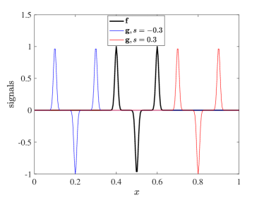
Problem statement. Let be a three-pulse signal given at discrete points , with , where
Here, is a given positive constant that controls the spread of the three pulses; the smaller , the narrower the three pulses. Let further be a shifted version of with a shift given at the same discrete points , with , where
Assuming , our goal is to find the “optimal” shift that minimizes the “distance” between the original signal and the shifted signal ,
Here, is a “loss” function that measures dissimilarities between and ; see the discussion below. While being a simple problem with a known solution , this model problem serves as an illustrative example exhibiting important challenges that we may face in solving optimization problems. Figure 4 shows the original signal and two shifted signals for two different shifts and . Wide signals (left) correspond to width , and narrow signals (right) correspond to width .

Loss functions. A first step is tackling an optimization problem is to select an appropriate loss function. Here, we consider and compare three loss functions:
-
•
Euclidean distance (or norm): .
-
•
Quadratic Wasserstein distance: defined in (29).
-
•
Quadratic Sinkhorn divergence: defined in (30).
It is to be noted that since the two signals are not necessarily probability vectors, i.e. positivity and mass balance are not expected, the signals need to be pre-processed before we can measure their Wasserstein distance and Sinkhorn divergence. While there are various techniques for this, here we employ a sign-splitting and normalization technique that considers the non-negative parts and and the non-positive parts and of the two signals separately. Precisely, we define
| (29) |
| (30) |
Two desirable properties of a loss function include its convexity with respect to the unknown parameter (here ) and its efficient computability for many different values of . While the Euclidean distance is widely used and can be efficiently computed with a cost , it may generate multiple local extrema that could result in converging to wrong solutions. The Wasserstein metric, on the other hand, features better convexity and hence better convergence to correct solutions; see [11] and references there in. However, the application of Wasserstein metric is limited to low-dimensional signals due to its high computational cost and infeasibility in high dimensions. This makes the Wasserstein loss function particularly suitable for one-dimensional problems, where it can be efficiently computed with a cost , as discussed in Section 2.1. As a promising alternative to and , we may consider the Sinkhorn loss function that possesses both desirable properties of a loss function. In terms of convexity, Sinkhorn divergence is similar to the Wasserstein metric. In terms of computational cost, as shown in the present work, we can efficiently compute Sinkhorn divergence in multiple dimensions with a near-linear cost .
Numerical results and discussion. Figure 5 shows the loss functions () versus . Here, we set and consider two different values for the width of signals, (left figure) and (right figure). We compute the Sinkhorn loss function with both by the original Sinkhorn’s algorithm (labeled in the figure) and by the proposed fast algorithm outlined in Algorithm 1 (labeled in the figure). In computing , we obtain the optimal local ranks by (26), with parameters and that correspond to the cost function with ; see the discussion on cost functions in Section 3.1 for this choice of parameters. We consider the accuracy tolerances .

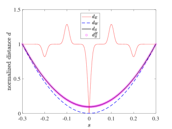
As we observe, the Euclidean loss function has local extrema, while the Wasserstein and Sinkhorn loss functions are convex. We also observe that well approximates , verifying the accuracy of the proposed algorithm in computing Sinkhorn divergence.
Figure 6 shows the CPU time of computing as a function of . We observe that the cost is as expected.

5 Conclusion
This work presents a fast method for computing Sinkhorn divergence between two discrete probability vectors supported on possibly high-dimensional spaces. The cost matrix in optimal transport problem is assumed to be decomposable into a sum of asymptotically smooth Kronecker product factors. The method combines Sinkhorn’s matrix scaling iteration with a low-rank hierarchical representation of the scaling matrices to achieve a near-linear complexity. This provides a fast and easy-to-implement algorithm for computing Sinkhorn divergence, enabling the applicability of Sinkhorn divergence to large-scale optimization problems, where the computation of classical Wasserstein metric is not feasible.
Future directions include exploring the application of the proposed hierarchical low-rank Sinkhorn’s algorithm to large-scale Bayesian inversion and other data science and machine learning problems.
Acknowledgments. I would like to thank Klas Modin for a question he raised during a seminar that I gave at Chalmers University of Technology in Gothenburg, Sweden. Klas’ question on the computation of Wasserstein metric in multiple dimensions triggered my curiosity and persuaded me to work further on the subject.
Appendix
In this appendix we collect a number of auxiliary lemmas.
Lemma 1.
For a real matrix , let denote the matrix obtained by the entrywise application of exponential function to , i.e. . Then we have
Proof.
The case is trivial. Consider the case . By the definition of Kronecker sum, we have
Now assume that it is true for :
Then
∎
Lemma 2.
We have
Proof.
The case is trivial. Consider the case . By the definition of Kronecker sum, we have
Now assume that it is true for :
Then
noting that , and and for .
∎
References
- [1] J. Altschuler, J. Weed, and P. Rigollet. Near-linear time approximation algorithms for optimal transport via Sinkhorn iteration. In I. Guyon, U. V. Luxburg, S. Bengio, H. Wallach, R. Fergus, S. Vishwanathan, and R. Garnett, editors, Advances in Neural Information Processing Systems 30, pages 1961–1971, 2017.
- [2] Y. Brenier. Polar factorization and monotone rearrangement of vector-valued functions. Comm. Pure Appl. Math., 44:375–417, 1991.
- [3] M. Cuturi. Sinkhorn distances: Lightspeed computation of optimal transport. In Advances in Neural Information Processing Systems 26, pages 2292–2300, 2013.
- [4] P. Dvurechensky, A. Gasnikov, and A. Kroshnin. Computational optimal transport: Complexity by accelerated gradient descent is better than by Sinkhorn’s algorithm. In J. Dy and A. Krause, editors, Proceedings of the 35th International Conference on Machine Learning, PMLR 80, pages 1367–1376, 2018.
- [5] B. Engquist, B.D. Froese Brittany, and Y. Yang. Optimal transport for seismic full waveform inversion. Communications in Mathematical Sciences, 14(8):2309–2330, 2016.
- [6] J. Franklin and J. Lorenz. On the scaling of multidimensional matrices. Linear Algebra and its Application, 114:717–735, 1989.
- [7] W. Hackbusch. Hierarchical Matrices: Algorithms and Analysis, volume 49 of Springer Series in Computational Mathematics. Springer-Verlag, 2015.
- [8] J. Indritz. An inequality for Hermite polynomials. Proc. Amer. Math. Soc., 12:981–983, 1961.
- [9] B. Kalantari and L. Khachiyan. On the complexity of nonnegative-matrix scaling. Linear Algebra and its Applications, 240:87–103, 1996.
- [10] P. A Knight. The Sinkhorn–Knopp algorithm: convergence and applications. SIAM J. on Matrix Analysis and Applications, 30:261–275, 2008.
- [11] M. Motamed and D. Appelö. Wasserstein metric-driven Bayesian inversion with applications to signal processing. International J. for Uncertainty Quantification, 9:395–414, 2019.
- [12] A. Nemirovski and U. Rothblum. On complexity of matrix scaling. Linear Algebra and its Applications, 302:435–460, 1999.
- [13] G. Peyré and M. Cuturi. Computational optimal transport. Foundations and Trends in Machine Learning, 11:355–607, 2019.
- [14] R. Sinkhorn. A relationship between arbitrary positive matrices and doubly stochastic matrices. Annals of Mathematical Statististics, 35:876–879, 1964.
- [15] J. Solomon, F. De Goes, G. Peyré, M. Cuturi, A. Butscher, A. Nguyen, T. Du, and L. Guibas. Convolutional Wasserstein distances: efficient optimal transportation on geometric domains. ACM Transactions on Graphics, 34:66:1–66:11, 2015.
- [16] C. Villani. Topics in Optimal Transportation, volume 58 of Graduate Studies in Mathematics. American Mathematical Society, 2003.
- [17] C. Villani. Optimal Transport: Old and New, volume 338 of Grundlehren der mathematischen Wissenschaften. Springer Verlag, 2009.
- [18] Y. Yang, B. Engquist, J. Sun, and B. F. Hamfeldt. Application of optimal transport and the quadratic Wasserstein metric to full-waveform inversion. Geophysics, 83(1):R43–R62, 2018.