This paper was converted on www.awesomepapers.org from LaTeX by an anonymous user.
Want to know more? Visit the Converter page.

Hierarchical Deep Counterfactual Regret Minimization

\nameJiayu Chen \email[email protected]
\addrPurdue University
West Lafayette, IN 47906 \AND\nameTian Lan \email[email protected]
\addrThe George Washington University
Washington, DC 20052 \AND\nameVaneet Aggarwal \email[email protected]
\addrPurdue University
West Lafayette, IN 47907
Abstract

Imperfect Information Games (IIGs) offer robust models for scenarios where decision-makers face uncertainty or lack complete information. Counterfactual Regret Minimization (CFR) has been one of the most successful family of algorithms for tackling IIGs. The integration of skill-based strategy learning with CFR could potentially mirror more human-like decision-making process and enhance the learning performance for complex IIGs. It enables the learning of a hierarchical strategy, wherein low-level components represent skills for solving subgames and the high-level component manages the transition between skills. In this paper, we introduce the first hierarchical version of Deep CFR (HDCFR), an innovative method that boosts learning efficiency in tasks involving extensively large state spaces and deep game trees. A notable advantage of HDCFR over previous works is its ability to facilitate learning with predefined (human) expertise and foster the acquisition of skills that can be transferred to similar tasks. To achieve this, we initially construct our algorithm on a tabular setting, encompassing hierarchical CFR updating rules and a variance-reduced Monte Carlo sampling extension. Notably, we offer the theoretical justifications, including the convergence rate of the proposed updating rule, the unbiasedness of the Monte Carlo regret estimator, and ideal criteria for effective variance reduction. Then, we employ neural networks as function approximators and develop deep learning objectives to adapt our proposed algorithms for large-scale tasks, while maintaining the theoretical support.

1 Introduction

Imperfect Information Games (IIGs) can be used to model various application domains where decision-makers have incomplete or uncertain information about the state of the environment, such as auctions (Noe et al. (2012)), diplomacy (Bakhtin et al. (2022)), cybersecurity (Kakkad et al. (2019)), etc. As one of the most successful family of algorithms for IIGs, variants of tabular Counterfactual Regret Minimization (CFR) (Zinkevich et al. (2007)) have been employed in all recent milestones of Poker AI which serves as a quintessential benchmark for IIGs (Bowling et al. (2015); Moravčík et al. (2017); Brown and Sandholm (2018)). However, implementing tabular CFR in domains characterized by an exceedingly large state space necessitates the use of abstraction techniques that group similar states together (Ganzfried and Sandholm (2014a); Sandholm (2015)), which requires extensive domain-specific expertise. To address this challenge, researchers have proposed deep learning extensions of CFR (Brown et al. (2019); Li et al. (2020); Steinberger et al. (2020)), which leverage neural networks as function approximations, enabling generalization across the state space.

On the other hand, professionals in a field typically possess robust domain-specific skills, which they can employ to compose comprehensive strategies for tackling diverse and intricate task scenarios. Therefore, integrating the skill-based strategy learning with CFR has the potential to enable human-like decision-making and enhance the learning performance for complex tasks with extended decision horizons, which is still an open problem. To accomplish this, the agent needs to learn a hierarchical strategy, in which the low-level components represent specific skills, and the high-level component coordinates the transition among skills. Notably, this is akin to the option framework (Sutton et al. (1999)) proposed in the context of reinforcement learning (RL), which enables learning or planning at multiple levels of temporal abstractions. Further, it’s worth noting that a hierarchical strategy is more interpretable, allowing humans to identify specific subcases where AI agents struggle. Targeted improvements can then be made by injecting critical skills that are defined by experts or learned through well-developed subgame-solving techniques (Moravcik et al. (2016); Brown and Sandholm (2017); Brown et al. (2018)). Also, skills acquired in one task, being more adaptable than the overarching strategy, can potentially be transferred to similar tasks to improve the learning in new IIGs.

In this paper, we introduce the first hierarchical extension of Deep CFR (HDCFR), a novel approach that significantly enhances learning efficiency in tasks with exceptionally large state spaces and deep game trees and enables learning with transferred knowledge. To achieve this, we establish the theoretical foundations of our algorithm in the tabular setting, drawing inspiration from vanilla CFR (Zinkevich et al. (2007)) and Variance-Reduced Monte Carlo CFR (VR-MCCFR) (Davis et al. (2020)). Then, building on these results, we introduce deep learning objectives to ensure the scalability of HDCFR. In particular, our contributions are as follows. (1) We propose to learn a hierarchical strategy for each player, which contains low-level strategies to encode skills (represented as sequences of primitive actions) and a high-level strategy for skill selection. We provide formal definitions for the hierarchical strategy within the IIG model, and provide extended CFR updating rules for strategy learning (i.e., HCFR) with convergence guarantees. (2) Vanilla CFR requires a perfect game tree model and a full traverse of the game tree in each training iteration, which can limit its use especially for large-scale tasks. Thus, we propose a sample-based model-free extension of HCFR, for which the key elements include unbiased Monte Carlo estimators of counterfactual regrets and a hierarchical baseline function for effective variance reduction. Note that controlling sample variance is vital for tasks with extended decision horizons, which our algorithm targets. Theoretical justifications are provided for each element of our design. (3) We present HDCFR, where the hierarchical strategy, regret, and baseline are approximated with Neural Networks, and the training objectives are demonstrated to be equivalent to those proposed in the tabular setting, i.e., (1) and (2), when optimality is achieved, thereby preserving the theoretical results while enjoying scalability.

2 Background

This section presents the background of our work, which includes two key concepts: Counterfactual Regret Minimization (CFR) and the option framework.

2.1 Counterfactual Regret Minimization

First, we introduce the extensive game model with imperfect information (Osborne and Rubinstein (1994)). In an extensive game, players make sequential moves represented by a game tree. At each non-terminal state, the player in control chooses from a set of available actions. At each terminal state, each player receives a payoff. In the presence of imperfect information, a player may not know which state they are in. For instance, in a poker game, a player sees its own cards and all cards laid on the table but not the opponents’ hands. Therefore, at each time step, each player makes decisions based on an information set – a collection of states that the controlling player cannot distinguish. Formally, the extensive game model can be represented by a tuple <N,H,A,P,σc,u,><N,H,A,P,\sigma_{c},u,\mathcal{I}>. NN is a finite set of players. HH is a set of histories, where each history is a sequence of actions of all players from the start of the game and corresponds to a game state. For h,hHh,h^{\prime}\in H, we write hhh\sqsubseteq h^{\prime} if hh is a prefix of hh^{\prime}. The set of actions available at hHh\in H is denoted as A(h)A(h). Suppose aA(h)a\in A(h), then (ha)H(ha)\in H a successor history of hh. Histories with no successors are terminal histories HTSHH_{TS}\subseteq H. P:H\HTSN{c}P:H\backslash H_{TS}\rightarrow N\cup\{c\} maps each non-terminal history to the player that chooses the next action, where cc is the chance player that acts according to a predefined distribution σc(|h)\sigma_{c}(\cdot|h). This chance player represents the environment’s inherent randomness, such as using a dice roll to decide the starting player. The utility function u:N×HTSu:N\times H_{TS}\rightarrow\mathbb{R} assigns a payoff for every player at each terminal history. For a player ii, i\mathcal{I}_{i} is a partition of {hH:P(h)=i}\{h\in H:P(h)=i\} and each element IiiI_{i}\in\mathcal{I}_{i} is an information set as introduced above. IiI_{i} also represents the observable information for ii shared by all histories hIih\in I_{i}. Due to the indistinguishability, we have A(h)=A(Ii),P(h)=P(Ii)A(h)=A(I_{i}),\ P(h)=P(I_{i}). Notably, our work focus on the two-player zero-sum setting, where N={1,2}N=\{1,2\} and u1(h)=u2(h),hHTSu_{1}(h)=-u_{2}(h),\ \forall\ h\in H_{TS}, like previous works on CFR (Zinkevich et al. (2007); Brown et al. (2019); Davis et al. (2020)).

Every player iNi\in N selects actions according to a strategy σi\sigma_{i} that maps each information set IiI_{i} to a distribution over actions in A(Ii)A(I_{i}). Note that σi(|h)=σi(|Ii),hIi\sigma_{i}(\cdot|h)=\sigma_{i}(\cdot|I_{i}),\ \forall\ h\in I_{i}. The learning target of CFR is a Nash Equilibrium (NE) strategy profile σ={σ1,σ2}\sigma^{*}=\{\sigma_{1}^{*},\sigma_{2}^{*}\}, where no player has an incentive to deviate from their specified strategy. That is, ui(σ)maxσiui({σi,σi}),iNu_{i}(\sigma^{*})\geq\max_{\sigma_{i}}u_{i}(\{\sigma_{i},\sigma_{-i}^{*}\}),\ \forall\ i\in{N}, where i-i represents the players other than ii, ui(σ)u_{i}(\sigma) is the expected payoff to player ii of σ\sigma and defined as follows:

ui(σ)=hHTSui(h)πσ(h),πσ(h)=(ha)hσP(h)(a|I(h))\displaystyle u_{i}(\sigma)=\sum_{h^{\prime}\in H_{TS}}u_{i}(h^{\prime})\pi^{\sigma}(h^{\prime}),\ \pi^{\sigma}(h^{\prime})=\prod_{(ha)\sqsubseteq h^{\prime}}\sigma_{P(h)}(a|I(h)) (1)

I(h)I(h) denotes the information set containing hh, and πσ(h)\pi^{\sigma}(h) is the reach probability of hh when employing σ\sigma. πσ(h)\pi^{\sigma}(h) can be decomposed as iN{c}πiσ(h)\prod_{i\in N\cup\{c\}}\pi_{i}^{\sigma}(h), where πiσ(h)=(ha)h,P(h)=iσi(a|I(h))\pi_{i}^{\sigma}(h)=\prod_{(ha)\sqsubseteq h^{\prime},P(h)=i}\sigma_{i}(a|I(h)). In addition, πσ(I)=hIπσ(h)\pi^{\sigma}(I)=\sum_{h\in I}\pi^{\sigma}(h) represents the reach probability of the information set II.

CFR proposed in Zinkevich et al. (2007) is an iterative algorithm which accumulates the counterfactual regret RiT(a|I)R_{i}^{T}(a|I) for each player ii at each information set IiI\in\mathcal{I}_{i}. This regret informs the strategy determination. RiT(a|I)R_{i}^{T}(a|I) is defined as follows:

RiT(a|I)=1Tt=1Tπiσt(I)(ui(σt|Ia,I)ui(σt,I))\displaystyle R_{i}^{T}(a|I)=\frac{1}{T}\sum_{t=1}^{T}\pi^{\sigma^{t}}_{-i}(I)(u_{i}(\sigma^{t}|_{I\rightarrow a},I)-u_{i}(\sigma^{t},I)) (2)
ui(σ,I)=hIπiσ(h)hHTSπσ(h,h)ui(h)/πiσ(I)\displaystyle u_{i}(\sigma,I)=\sum_{h\in I}\pi_{-i}^{\sigma}(h)\sum_{h^{\prime}\in H_{TS}}\pi^{\sigma}(h,h^{\prime})u_{i}(h^{\prime})/\pi^{\sigma}_{-i}(I)

where σt\sigma^{t} is the strategy profile at iteration tt, σt|Ia\sigma^{t}|_{I\rightarrow a} is identical to σt\sigma^{t} except that the player always chooses the action aa at II, πσ(h,h)\pi^{\sigma}(h,h^{\prime}) denotes the reach probability from hh to hh^{\prime} which equals πσ(h)πσ(h)\frac{\pi^{\sigma}(h^{\prime})}{\pi^{\sigma}(h)} if hhh\sqsubseteq h^{\prime} and 0 otherwise. Intuitively, RiT(a|I)R_{i}^{T}(a|I) represents the expected regret of not choosing action aa at II. With RiT(a|I)R_{i}^{T}(a|I), the next strategy profile σiT+1(|I)\sigma^{T+1}_{i}(\cdot|I) is acquired with regret matching (Abernethy et al. (2011)), which sets probabilities proportional to the positive regrets: σiT+1(a|I)max(RiT(a|I),0)\sigma^{T+1}_{i}(a|I)\propto\max(R_{i}^{T}(a|I),0). Defining the average strategy σ¯iT(|I)\overline{\sigma}^{T}_{i}(\cdot|I) such that σ¯iT(a|I)t=1Tπiσt(I)σit(a|I)\overline{\sigma}^{T}_{i}(a|I)\propto\sum_{t=1}^{T}\pi_{i}^{\sigma^{t}}(I)\sigma^{t}_{i}(a|I), CFR guarantees that the strategy profile σ¯T={σ¯iT|iN}\overline{\sigma}^{T}=\{\overline{\sigma}^{T}_{i}|i\in N\} converges to a Nash Equilibrium as TT\rightarrow\infty.

2.2 The Option Framework

As proposed in Sutton et al. (1999), an option z𝒵z\in\mathcal{Z} can be described with three components: an initiation set Initz𝒮Init_{z}\subseteq\mathcal{S}, an intra-option policy σz(a|s):𝒮×𝒜[0,1]\sigma_{z}(a|s):\mathcal{S}\times\mathcal{A}\rightarrow[0,1], and a termination function βz(s):𝒮[0,1]\beta_{z}(s):\mathcal{S}\rightarrow[0,1]. 𝒮\mathcal{S}, 𝒜\mathcal{A}, 𝒵\mathcal{Z} represent the state, action, option space, respectively. An option zz is available in state ss if and only if sInitzs\in Init_{z}. Once the option is taken, actions are selected according to σz\sigma_{z} until it terminates stochastically according to βz\beta_{z}, i.e., the termination probability at the current state. A new option will be activated by a high-level policy σ𝒵(z|s):𝒮×𝒵[0,1]\sigma_{\mathcal{Z}}(z|s):\mathcal{S}\times\mathcal{Z}\rightarrow[0,1] once the previous option terminates. In this way, σ𝒵(z|s)\sigma_{\mathcal{Z}}(z|s) and σz(a|s)\sigma_{z}(a|s) constitute a hierarchical policy for a certain task. Hierarchical policies tend to have superior performance on complex long-horizon tasks which can be broken down into and processed as a series of subtasks.

The one-step option framework (Li et al. (2021a)) is proposed to learn the hierarchical policy without the extra need to justify the exact beginning and breaking condition of each option, i.e., InitzInit_{z} and βz\beta_{z}. First, it assumes that each option is available at each state, i.e., Initz=𝒮,z𝒵Init_{z}=\mathcal{S},\forall\ z\in\mathcal{Z}. Second, it redefines the high-level and low-level policies as σH(z|s,z)\sigma^{H}(z|s,z^{\prime}) (zz^{\prime}: the option in the previous timestep) and σL(a|s,z)\sigma^{L}(a|s,z), respectively, and implementing them as end-to-end neural networks. In particular, the Multi-Head Attention (MHA) mechanism (Vaswani et al. (2017)) is adopted in σH(z|s,z)\sigma^{H}(z|s,z^{\prime}), which enables it to temporally extend options in the absence of the termination function βz\beta_{z}. Intuitively, if zz^{\prime} still fits ss, σH(z|s,z)\sigma^{H}(z|s,z^{\prime}) will assign a larger attention weight to zz^{\prime} and thus has a tendency to continue with it; otherwise, a new option with better compatibility will be sampled. Then, the option is sampled at each timestep rather than after the previous option terminates. With this simplified framework, we only need to train the hierarchical policy, i.e., σH\sigma^{H} and σL\sigma^{L}.

The option framework is proposed within the realm of RL as opposed to CFR; however, these two fields are closely related. The authors of (Srinivasan et al. (2018); Fu et al. (2022)) propose actor-critic algorithms for multi-agent adversarial games with partial observability and show that they are indeed a form of MCCFR for IIGs. This insight inspires our adoption of the one-step option framework to create a hierarchical extension for CFR.

3 Methodology

In this work, we aim at extending CFR to learn a hierarchical strategy in the form of Neural Networks (NNs) to solve IIGs with extensive state spaces and deep game trees. The high-level and low-level strategies serve distinct roles in the learning system, where low-level components represent various skills composed of primitive actions, and the high-level component orchestrates their utilization, thus they should be defined and learned as different functions. In the absence of prior research on hierarchical extensions of CFR, we establish our work’s theoretical foundations by drawing upon tabular CFR algorithms. Firstly, we define the hierarchical strategy and hierarchical counterfactual regret, and provide corresponding updating rules along with the convergence guarantee. Subsequently, we propose that an unbiased estimation of the hierarchical counterfactual regret can be achieved through Monte Carlo sampling (Lanctot et al. (2009)) and that the sample variance can be reduced by introducing a hierarchical baseline function. This Low-Variance Monte Carlo sampling extension enables our algorithm to to tackle domains with vast or unknown game trees (i.e., the model-free setting) - where standard CFR traversal is impractical - without compromising the convergence rate. Finally, with the theoretical foundations established in the tabular setting, we develop our algorithm, HDCFR, by approximating these hierarchical functions using NNs and training them with novel objective functions. These training objectives are demonstrated to be consistent with the updating rules in the tabular case when optimality is achieved, thereby the theoretical support is maintained.

3.1 Preliminaries

At a game state hh, the player ii makes its tt-th decision by selecting a hierarchical action a~t(zt,at)\widetilde{a}_{t}\triangleq(z_{t},a_{t}), i.e., the option (a.k.a., skill) and primitive action, based on the observable information for player ii at hh, including the private observations o1:to_{1:t} and decision sequence a~1:(t1)\widetilde{a}_{1:(t-1)} of player ii, and the public information for all players (defined by the game). All histories that share the same observable information are considered indistinguishable to player ii and belong to the same information set IiI_{i}. Thus, in this work, we also use IiI_{i} to denote observations upon which player ii makes decisions. With the hierarchical actions, we can redefine the extensive game model as <N,H,A~,P,σc,u,><N,H,\widetilde{A},P,\sigma_{c},u,\mathcal{I}>. Here, NN, PP, uu, and \mathcal{I} retain the definitions in Section 2.1. HH includes all the possible histories, each of which is a sequence of hierarchical actions of all players starting from the first time step. A~(h)=Z(h)×A(h)\widetilde{A}(h)=Z(h)\times A(h), where Z(h)Z(h) and A(h)A(h) represent the options and primitive actions available at hh respectively. σc((zc,a)|h)=σc(a|h)\sigma_{c}((z_{c},a)|h)=\sigma_{c}(a|h), where σc(a|h)\sigma_{c}(a|h) is the predefined distribution in the original game model and zcz_{c} (a dummy variable) is the only option choice for the chance player.

The learning target for player ii is a hierarchical strategy σi(a~t|Ii)\sigma_{i}(\widetilde{a}_{t}|I_{i}), which, by the chain rule, can be decomposed as σiH(zt|Ii)σiL(at|Ii,zt)\sigma_{i}^{H}(z_{t}|I_{i})\cdot\sigma_{i}^{L}(a_{t}|I_{i},z_{t}). Note that although IiI_{i} includes z1:t1z_{1:t-1}, we follow the conditional independence assumption of the one-step option framework (Li et al. (2021a); Zhang and Whiteson (2019)) which states that ztz1:(t2)|zt1z_{t}\perp\!\!\!\perp z_{1:(t-2)}\ |\ z_{t-1} and atz1:(t1)|zta_{t}\perp\!\!\!\perp z_{1:(t-1)}\ |\ z_{t}, thus only zt1z_{t-1} (ztz_{t}) is used for σiH\sigma_{i}^{H} (σiL\sigma_{i}^{L}) to determine ztz_{t} (ata_{t}). With the hierarchical strategy, we can redefine the expected payoff and reach probability in Equation (1) by simply substituting aa with a~\widetilde{a}, based on which we have the definition of the average overall regret of player ii at iteration TT: (From this point forward, tt refers to a certain learning iteration rather than a time step within an iteration.)

Rfull,iT=1Tmaxσit=1T(ui({σi,σit})ui(σt))\displaystyle R_{full,i}^{T}=\frac{1}{T}\max_{\sigma_{i}^{{}^{\prime}}}\sum_{t=1}^{T}(u_{i}(\{\sigma_{i}^{{}^{\prime}},\sigma_{-i}^{t}\})-u_{i}(\sigma^{t})) (3)

The following theorem (Theorem 2 from Zinkevich et al. (2007)) provides a connection between the average overall regret and the Nash Equilibrium solution.

Theorem 1

In a two-player zero-sum game at time TT, if both players’ average overall regret is less than ϵ\epsilon, then σ¯T={σ¯1T,σ¯2T}\overline{\sigma}^{T}=\{\overline{\sigma}^{T}_{1},\overline{\sigma}^{T}_{2}\} is a 2ϵ2\epsilon-Nash Equilibrium.

Here, the average strategy σ¯iT\overline{\sigma}^{T}_{i} is defined as (iN,Ii,a~A~(I)\forall\ i\in N,I\in\mathcal{I}_{i},\widetilde{a}\in\widetilde{A}(I)):

σ¯iT(a~|I)=(Σt=1Tπiσt(I)σit(a~|I))/Σt=1Tπiσt(I)\displaystyle\overline{\sigma}^{T}_{i}(\widetilde{a}|I)=\left(\Sigma_{t=1}^{T}\pi_{i}^{\sigma^{t}}(I)\sigma^{t}_{i}(\widetilde{a}|I)\right)/\Sigma_{t=1}^{T}\pi_{i}^{\sigma^{t}}(I) (4)

An ϵ\epsilon-Nash Equilibrium σ\sigma approximates a Nash Equilibrium, with the property that ui(σ)+ϵmaxσiui({σi,σi}),iNu_{i}(\sigma)+\epsilon\geq\max_{\sigma_{i}^{{}^{\prime}}}u_{i}(\{\sigma_{i}^{{}^{\prime}},\sigma_{-i}\}),\ \forall\ i\in{N}. Thus, ϵ\epsilon measures the distance of σ\sigma to the Nash Equilibrium in expected payoff. Then, according to Theorem 1, as Rfull,iT0R_{full,i}^{T}\rightarrow 0 (iN\forall\ i\in N), σ¯T\overline{\sigma}^{T} converges to NE. Notably, Theorem 1 can be applied directly to our hierarchical setting, as the only difference from the original setting related to Theorem 1 is the replacement of aa with a~\widetilde{a} in Rfull,iTR_{full,i}^{T} and σ¯iT(a~|I)\overline{\sigma}^{T}_{i}(\widetilde{a}|I). This difference can be viewed as employing a new action space (i.e., AA~A\rightarrow\widetilde{A}) and is independent of using the option framework (i.e., the hierarchical extension).

3.2 Hierarchical Counterfactual Regret Minimization

One straightforward way to learn a hierarchical strategy σi(a~|I)=σiH(z|I)σiL(a|I,z)\sigma_{i}(\widetilde{a}|I)=\sigma_{i}^{H}(z|I)\cdot\sigma_{i}^{L}(a|I,z) is to view σi(a~|I)\sigma_{i}(\widetilde{a}|I) as a unified strategy defined on a new action set A~\widetilde{A}, and then apply CFR directly to learn it. However, this approach does not allow for the explicit separation and utilization of the high-level and low-level components, such as extracting and reusing skills (i.e., low-level parts) or initializing them with human knowledge. In this section, we treat σiH\sigma_{i}^{H} and σiL\sigma_{i}^{L} as distinct functions and introduce Hierarchical CFR (HCFR) to separately learn σiH(z|I)\sigma_{i}^{H}(z|I) and σiL(a|I,z),Ii,zZ(I),aA(I)\sigma_{i}^{L}(a|I,z),\forall\ I\in\mathcal{I}_{i},z\in Z(I),a\in A(I). Additionally, we provide the convergence guarantee for HCFR.

Taking inspiration from CFR (Zinkevich et al. (2007)), we derive an upper bound for the average overall regret Rfull,iTR_{full,i}^{T}, which is given by the sum of high-level and low-level counterfactual regrets at each information set, namely RiT,H(z|I)R^{T,H}_{i}(z|I) and RiT,L(a|I,z)R^{T,L}_{i}(a|I,z). In this way, we can minimize RiT,H(z|I)R^{T,H}_{i}(z|I) and RiT,L(a|I,z)R^{T,L}_{i}(a|I,z) for each individual IiI\in\mathcal{I}_{i} independently by adjusting σiH(z|I)\sigma_{i}^{H}(z|I) and σiL(a|I,z)\sigma_{i}^{L}(a|I,z) respectively, and in doing so, minimize the average overall regret. The learning of the high-level and low-level strategy is also decoupled.

Theorem 2

With the following definitions of high-level and low-level counterfactual regrets:

RiT,H(z|I)=1Tt=1Tπiσt(I)(ui(σt|Iz,I)ui(σt,I)),RiT,H(I)=maxzZ(I)RiT,H(z|I)\displaystyle\ \ \ \ \ \ \ \ R^{T,H}_{i}(z|I)=\frac{1}{T}\sum_{t=1}^{T}\pi^{\sigma^{t}}_{-i}(I)(u_{i}(\sigma^{t}|_{I\rightarrow z},I)-u_{i}(\sigma^{t},I)),\ R^{T,H}_{i}(I)=\max_{z\in Z(I)}R^{T,H}_{i}(z|I) (5)
RiT,L(a|I,z)=1Tt=1Tπiσt(I)(ui(σt|Iza,Iz)ui(σt,Iz)),RiT,L(I,z)=maxaA(I)RiT,L(a|I,z)\displaystyle R^{T,L}_{i}(a|I,z)=\frac{1}{T}\sum_{t=1}^{T}\pi^{\sigma^{t}}_{-i}(I)(u_{i}(\sigma^{t}|_{Iz\rightarrow a},Iz)-u_{i}(\sigma^{t},Iz)),\ R^{T,L}_{i}(I,z)=\max_{a\in A(I)}R^{T,L}_{i}(a|I,z)

we have Rfull,iTIi[Ri,+T,H(I)+zZ(I)Ri,+T,L(I,z)]R_{full,i}^{T}\leq\sum_{I\in\mathcal{I}_{i}}\left[R^{T,H}_{i,+}(I)+\sum_{z\in Z(I)}R^{T,L}_{i,+}(I,z)\right].

Here, Ri,+T,H(I)=max(RiT,H(I),0),Ri,+T,L(I,z)=max(RiT,L(I,z),0)R^{T,H}_{i,+}(I)=\max(R^{T,H}_{i}(I),0),\ R^{T,L}_{i,+}(I,z)=\max(R^{T,L}_{i}(I,z),0), ui(σt,Iz)u_{i}(\sigma^{t},Iz) is the expected payoff for choosing option zz at II, σt|Iza\sigma^{t}|_{Iz\rightarrow a} is a hierarchical strategy profile identical to σt\sigma^{t} except that the intra-option (i.e., low-level) strategy of option zz at II is always choosing aa. Detailed proof of Theorem 2 is available in Appendix A.

After obtaining RiT,HR^{T,H}_{i} and RiT,LR^{T,L}_{i}, we can compute the high-level and low-level strategies for the next iteration as follows: (iN,Ii,zZ(I),aA(I)\forall\ i\in N,I\in\mathcal{I}_{i},z\in Z(I),a\in A(I))

σiT+1,H(z|I)={Ri,+T,H(z|I)/μH,μH>0,1/|Z(I)|,o\w.μH=zZ(I)Ri,+T,H(z|I)\displaystyle\ \ \ \ \sigma_{i}^{T+1,H}(z|I)=\left\{\begin{aligned} R^{T,H}_{i,+}(z|I)/\mu^{H}&,&\mu^{H}>0,\\ 1/|Z(I)|&,&o\backslash w.\end{aligned}\right.\ \ \ \ \mu^{H}=\sum_{z^{\prime}\in Z(I)}R^{T,H}_{i,+}(z^{\prime}|I) (6)
σiT+1,L(a|I,z)={Ri,+T,L(a|I,z)/μL,μL>0,1/|A(I)|,o\w.μL=aA(I)Ri,+T,L(a|I,z)\displaystyle\sigma_{i}^{T+1,L}(a|I,z)=\left\{\begin{aligned} R^{T,L}_{i,+}(a|I,z)/\mu^{L}&,&\mu^{L}>0,\\ 1/|A(I)|&,&o\backslash w.\end{aligned}\right.\ \ \ \ \mu^{L}=\sum_{a^{\prime}\in A(I)}R^{T,L}_{i,+}(a^{\prime}|I,z)

In this way, the counterfactual regrets and strategies are calculated alternatively (i.e., σ1:tRtσt+1,σ1:t+1Rt+1σt+2,\sigma^{1:t}\rightarrow R^{t}\rightarrow\sigma^{t+1},\ \sigma^{1:t+1}\rightarrow R^{t+1}\rightarrow\sigma^{t+2},\ \cdots) with Equation (5) and (6) for iterations until convergence (i.e., Rfull,iT0R_{full,i}^{T}\rightarrow 0). The convergence rate of this algorithm is presented in the following theorem:

Theorem 3

If player ii selects options and actions according to Equation (6), then Rfull,iTΔu,i|i|(|Zi|+|Zi||Ai|)/TR_{full,i}^{T}\leq\Delta_{u,i}|\mathcal{I}_{i}|(\sqrt{|Z_{i}|}+|Z_{i}|\sqrt{|A_{i}|})/\sqrt{T}, where Δu,i=maxhHTSui(h)minhHTSui(h)\Delta_{u,i}=\max_{h^{\prime}\in H_{TS}}u_{i}(h^{\prime})-\min_{h^{\prime}\in H_{TS}}u_{i}(h^{\prime}), |i||\mathcal{I}_{i}| is the number of information sets for player ii, |Ai|=maxh:P(h)=i|A(h)||A_{i}|=\max_{h:P(h)=i}|A(h)|, |Zi|=maxh:P(h)=i|Z(h)||Z_{i}|=\max_{h:P(h)=i}|Z(h)|.

Thus, as TT\rightarrow\infty, Rfull,iT0R_{full,i}^{T}\rightarrow 0. Additionally, the convergence rate is 𝒪(T0.5)\mathcal{O}(T^{-0.5}), which is the same as CFR (Zinkevich et al. (2007)). Thus, the introduction of the option framework does not compromise the convergence guarantee, while allowing skill-based strategy learning. The proof of Theorem 3 is provided in Appendix B.

With σit,H\sigma^{t,H}_{i} and σit,L\sigma^{t,L}_{i}, we can compute the average high-level and low-level strategies as:

σ¯iT,H(z|I)=Σt=1Tπiσt(I)σit,H(z|I)Σt=1Tπiσt(I),σ¯iT,L(a|I,z)=Σt=1Tπiσt(Iz)σit,L(a|I,z)Σt=1Tπiσt(Iz)\displaystyle\overline{\sigma}^{T,H}_{i}(z|I)=\frac{\Sigma_{t=1}^{T}\pi_{i}^{\sigma^{t}}(I)\sigma^{t,H}_{i}(z|I)}{\Sigma_{t=1}^{T}\pi_{i}^{\sigma^{t}}(I)},\ \ \ \ \overline{\sigma}^{T,L}_{i}(a|I,z)=\frac{\Sigma_{t=1}^{T}\pi_{i}^{\sigma^{t}}(Iz)\sigma^{t,L}_{i}(a|I,z)}{\Sigma_{t=1}^{T}\pi_{i}^{\sigma^{t}}(Iz)} (7)

where πiσt(Iz)=πiσt(I)σit,H(z|I)\pi_{i}^{\sigma^{t}}(Iz)=\pi_{i}^{\sigma^{t}}(I)\sigma_{i}^{t,H}(z|I). Then, we can state:

Proposition 1

If both players sequentially use their average high-level and low-level strategies following the one-step option model, i.e., Ii\forall\ I\in\mathcal{I}_{i}, selecting an option zz according to σ¯iT,H(|I)\overline{\sigma}^{T,H}_{i}(\cdot|I) and then selecting the action aa according to the corresponding intra-option strategy σ¯iT,L(|I,z)\overline{\sigma}^{T,L}_{i}(\cdot|I,z), the resulting strategy profile converges to a Nash Equilibrium as TT\rightarrow\infty.

The proof is based on Theorem 1, for which you can refer to Appendix C.

3.3 Low-Variance Monte Carlo Sampling Extension

In vanilla CFR, counterfactual regrets and immediate strategies are updated for every information set during each iteration. This necessitates a complete traversal of the game tree, which becomes infeasible for large-scale game models. Monte Carlo CFR (MCCFR) (Lanctot et al. (2009)) is a framework that allows CFR to only update regrets/strategies on part of the tree for a single agent (i.e., the traverser) at each iteration. MCCFR features two sampling scheme variants: External Sampling (ES) and Outcome Sampling (OS). In OS, regrets/strategies are updated for information sets within a single trajectory that is generated by sampling one action at each decision point. In ES, a single action is sampled for non-traverser agents, while all actions of the traverser are explored, leading to updates over multiple trajectories. ES relies on perfect game models for backtracking and becomes impractical as the horizon increases, with which the search breadth grows exponentially. Our algorithm is specifically designed for domains with deep game trees, leading us to adopt OS as the sampling scheme. Nevertheless, OS is challenged by high sample variance, an issue that exacerbates with an increasing decision-making horizon. Therefore, in this section, we further complete our algorithm with a low-variance outcome sampling extension.

MCCFR’s main insight is substituting the counterfactual regrets RiTR^{T}_{i} with unbiased estimations, while maintaining the other learning rules (as in Section 3.2). This allows for updating functions only on information sets within the sampled trajectories, bypassing the need to traverse the full game tree. With MCCFR, the average overall regret Rfull,iT0R_{full,i}^{T}\rightarrow 0 as TT\rightarrow\infty at the same convergence rate as vanilla CFR, with high probability, as stated in Theorem 5 of Lanctot et al. (2009). Therefore, to apply the Monte Carlo extension, we propose unbiased estimations of RiT,H(z|I)R^{T,H}_{i}(z|I) and RiT,L(a|I,z)R^{T,L}_{i}(a|I,z), iN,Ii,zZ(I),aA(I)\forall\ i\in N,I\in\mathcal{I}_{i},z\in Z(I),a\in A(I).

First, we define RiT,H(z|I)R^{T,H}_{i}(z|I) and RiT,L(a|I,z)R^{T,L}_{i}(a|I,z) with the immediate counterfactual regrets ritr^{t}_{i} and values vitv_{i}^{t}: (vit,H(σt,h)=ui(h),hHTSv^{t,H}_{i}(\sigma^{t},h)=u_{i}(h),\ \forall\ h\in H_{TS})

RiT,H(z|I)=1Tt=1Trit,H(I,z),rit,H(I,z)=hIπiσt(h)[vit,L(σt,hz)vit,H(σt,h)]\displaystyle\quad\ R_{i}^{T,H}(z|I)=\frac{1}{T}\sum_{t=1}^{T}r_{i}^{t,H}(I,z),\ r_{i}^{t,H}(I,z)=\sum_{h\in I}\pi_{-i}^{\sigma^{t}}(h)\left[v^{t,L}_{i}(\sigma^{t},hz)-v^{t,H}_{i}(\sigma^{t},h)\right] (8)
RiT,L(a|I,z)=1Tt=1Trit,L(Iz,a),rit,L(Iz,a)=hIπiσt(h)[vit,H(σt,hza)vit,L(σt,hz)]\displaystyle R_{i}^{T,L}(a|I,z)=\frac{1}{T}\sum_{t=1}^{T}r_{i}^{t,L}(Iz,a),\ r_{i}^{t,L}(Iz,a)=\sum_{h\in I}\pi_{-i}^{\sigma^{t}}(h)\left[v^{t,H}_{i}(\sigma^{t},hza)-v^{t,L}_{i}(\sigma^{t},hz)\right]
vit,H(σt,h)=zZ(h)σP(h)t,H(z|h)vit,L(σt,hz),vit,L(σt,hz)=aA(h)σP(h)t,L(a|h,z)vit,H(σt,hza)\displaystyle v^{t,H}_{i}(\sigma^{t},h)=\sum_{z\in Z(h)}\sigma^{t,H}_{P(h)}(z|h)v_{i}^{t,L}(\sigma^{t},hz),\ v_{i}^{t,L}(\sigma^{t},hz)=\sum_{a\in A(h)}\sigma^{t,L}_{P(h)}(a|h,z)v^{t,H}_{i}(\sigma^{t},hza)

The equivalence between Equation (8) and (5) is proved in Appendix D.

Next, we propose to collect trajectories hHTSh^{\prime}\in H_{TS} with the sample strategy qtq^{t} at each iteration tt, and compute the corresponding sampled immediate counterfactual regrets r^it\hat{r}^{t}_{i} and values v^it\hat{v}_{i}^{t} as follows:

r^it,H(I,z|h)=hIπiσt(h)πqt(h)[v^it,H(σt,h,z|h)v^it,H(σt,h|h)]\displaystyle\ \ \hat{r}_{i}^{t,H}(I,z|h^{\prime})=\sum_{h\in I}\frac{\pi_{-i}^{\sigma^{t}}(h)}{\pi^{q^{t}}(h)}\left[\hat{v}^{t,H}_{i}(\sigma^{t},h,z|h^{\prime})-\hat{v}^{t,H}_{i}(\sigma^{t},h|h^{\prime})\right] (9)
r^it,L(Iz,a|h)=hIπiσt(h)πqt(hz)[v^it,L(σt,hz,a|h)v^it,L(σt,hz|h)]\displaystyle\hat{r}_{i}^{t,L}(Iz,a|h^{\prime})=\sum_{h\in I}\frac{\pi_{-i}^{\sigma^{t}}(h)}{\pi^{q^{t}}(hz)}\left[\hat{v}^{t,L}_{i}(\sigma^{t},hz,a|h^{\prime})-\hat{v}^{t,L}_{i}(\sigma^{t},hz|h^{\prime})\right]

Here, inspired by Davis et al. (2020), v^it,H(σt,h,z|h)\hat{v}^{t,H}_{i}(\sigma^{t},h,z|h^{\prime}) and v^it,L(σt,hz,a|h)\hat{v}^{t,L}_{i}(\sigma^{t},hz,a|h^{\prime}) are incorporated with the baseline function bitb^{t}_{i} for variance reduction: (v^it,H(σt,h|h)=ui(h)\hat{v}^{t,H}_{i}(\sigma^{t},h^{\prime}|h^{\prime})=u_{i}(h^{\prime}))

v^it,H(σt,h,z|h)=δ(hzh)qt(z|h)[v^it,L(σt,hz|h)bit(h,z)]+bit(h,z)\displaystyle\quad\ \ \hat{v}^{t,H}_{i}(\sigma^{t},h,z|h^{\prime})=\frac{\delta(hz\sqsubseteq h^{\prime})}{q^{t}(z|h)}\left[\hat{v}^{t,L}_{i}(\sigma^{t},hz|h^{\prime})-b_{i}^{t}(h,z)\right]+b^{t}_{i}(h,z) (10)
v^it,L(σt,hz,a|h)=δ(hzah)qt(a|h,z)[v^it,H(σt,hza|h)bit(h,z,a)]+bit(h,z,a)\displaystyle\hat{v}^{t,L}_{i}(\sigma^{t},hz,a|h^{\prime})=\frac{\delta(hza\sqsubseteq h^{\prime})}{q^{t}(a|h,z)}\left[\hat{v}^{t,H}_{i}(\sigma^{t},hza|h^{\prime})-b^{t}_{i}(h,z,a)\right]+b^{t}_{i}(h,z,a)

where δ()\delta(\cdot) is the indicator function. Accordingly, v^it,H(σt,h|h)\hat{v}^{t,H}_{i}(\sigma^{t},h|h^{\prime}) and v^it,L(σt,hz|h)\hat{v}^{t,L}_{i}(\sigma^{t},hz|h^{\prime}) are defined as zZ(h)σP(h)t,H(z|h)v^it,H(σt,h,z|h)\sum_{z\in Z(h)}\sigma^{t,H}_{P(h)}(z|h)\hat{v}_{i}^{t,H}(\sigma^{t},h,z|h^{\prime}) and aA(h)σP(h)t,L(a|h,z)v^it,L(σt,hz,a|h)\sum_{a\in A(h)}\sigma^{t,L}_{P(h)}(a|h,z)\hat{v}_{i}^{t,L}(\sigma^{t},hz,a|h^{\prime}). (For superscripts on r^\hat{r} and v^\hat{v}: use HH when the agent is in state hh or hzahza for high-level option choices, and LL in state hzhz for low-level action decisions.)

Regarding estimators proposed in Equation (9) and (10), we have the following theorems:

Theorem 4

For all iN,Ii,zZ(I),aA(I)i\in N,\ I\in\mathcal{I}_{i},\ z\in Z(I),\ a\in A(I), we have:

𝔼hπqt()[r^it,H(I,z|h)]=rit,H(I,z),𝔼hπqt()[r^it,L(Iz,a|h)]=rit,L(Iz,a)\displaystyle\mathbb{E}_{h^{\prime}\sim\pi^{q^{t}}(\cdot)}\left[\hat{r}_{i}^{t,H}(I,z|h^{\prime})\right]=r^{t,H}_{i}(I,z),\ \mathbb{E}_{h^{\prime}\sim\pi^{q^{t}}(\cdot)}\left[\hat{r}_{i}^{t,L}(Iz,a|h^{\prime})\right]=r^{t,L}_{i}(Iz,a) (11)

Therefore, we can acquire unbiased estimations of RiTR^{T}_{i} by substituting ritr_{i}^{t} with r^it\hat{r}^{t}_{i} in Equation (8). This theorem is proved in Appendix E. Notably, Theorem 4 doesn’t prescribe any specific form for the baseline function bitb^{t}_{i}. Yet, the baseline design can affect the sample variance of these unbiased estimators. As posited in Gibson et al. (2012), given a fixed ϵ>0\epsilon>0, estimators with reduced variance necessitate fewer iterations to converge to an ϵ\epsilon-Nash equilibrium. Hence, we propose the following ideal criteria for the baseline function to minimize the sample variance:

Theorem 5

If bit(h,z,a)=vit,H(σt,hza)b^{t}_{i}(h,z,a)=v^{t,H}_{i}(\sigma^{t},hza) and bit(h,z)=vit,L(σt,hz)b^{t}_{i}(h,z)=v^{t,L}_{i}(\sigma^{t},hz), for all hH\HTS,zZ(h),aA(h)h\in H\backslash H_{TS},\ z\in Z(h),\ a\in A(h), we have:

Varh[v^it,H(σt,h,z|h)|hh]=Varh[v^it,L(σt,hz,a|h)|hhz]=0\displaystyle{\rm Var}_{h^{\prime}}\left[\hat{v}_{i}^{t,H}(\sigma^{t},h,z|h^{\prime})|h^{\prime}\sqsupseteq h\right]={\rm Var}_{h^{\prime}}\left[\hat{v}_{i}^{t,L}(\sigma^{t},hz,a|h^{\prime})|h^{\prime}\sqsupseteq hz\right]=0 (12)

Consequently, Varhπqt()[r^it,H(I,z|h)]{\rm Var}_{h^{\prime}\sim\pi^{q^{t}}(\cdot)}\left[\hat{r}_{i}^{t,H}(I,z|h^{\prime})\right] and Varhπqt()[r^it,L(Iz,a|h)]{\rm Var}_{h^{\prime}\sim\pi^{q^{t}}(\cdot)}\left[\hat{r}_{i}^{t,L}(Iz,a|h^{\prime})\right] are minimized with respect to bitb^{t}_{i} for all IiI\in\mathcal{I}_{i}, zZ(I)z\in Z(I), aA(I)a\in A(I).

The proof can be found in Appendix F. The ideal criteria for the baseline function proposed in Theorem 5 is incorporated into our objective design in Section 3.4.

To sum up, by employing the immediate counterfactual regret estimators shown as Equation (9) and (10), and making appropriate choices for the baseline function (introduced in Section 3.4), we are able to bolster the adaptability and learning efficiency of our method through a low-variance outcome Monte Carlo sampling extension.

3.4 Hierarchical Deep Counterfactual Regret Minimization

Building upon theoretical foundations discussed in Section 3.2 and 3.3, we now present our algorithm – HDCFR. While the algorithm outline is similar to tabular CFR algorithms (Kakkad et al. (2019); Davis et al. (2020)), HDCFR differentiates itself by introducing NNs as function approximators for the counterfactual regret RitR_{i}^{t}, average strategy σ¯iT\overline{\sigma}^{T}_{i}, and baseline bitb^{t}_{i}. These approximations enable HDCFR to handle large-scale state spaces and are trained with specially-designed objective functions. In this section, we introduce the deep learning objectives, demonstrate their alignment with the theoretical underpinnings provided in Section 3.2 and 3.3, and then present the complete algorithm in pseudo-code form.

Three types of networks are trained: the counterfactual regret networks Ri,θt,H,Ri,θt,LR^{t,H}_{i,\theta},\ R^{t,L}_{i,\theta}, average strategy networks σ¯i,ϕT,H,σ¯i,ϕT,L\overline{\sigma}^{T,H}_{i,\phi},\ \overline{\sigma}^{T,L}_{i,\phi}, and baseline network btb^{t}. Notably, we do not maintain the counterfactual values v^t\hat{v}^{t} and baselines btb^{t} for each player. Instead, we leverage the property of two-player zero-sum games where the payoff of the two players offsets each other. Thus, we track the payoff for player 1 and use the opposite value as the payoff for player 2. That is, bt=b1t=b2tb^{t}=b^{t}_{1}=-b^{t}_{2}, vt=v1t=v2tv^{t}=v^{t}_{1}=-v^{t}_{2}.

First, the counterfactual regret networks are trained by minimizing the following two objectives, denoted as R,it,H\mathcal{L}^{t,H}_{R,i} and R,it,L\mathcal{L}^{t,L}_{R,i}, respectively.

𝔼(I,r^it,H)τRi[zZ(I)(Ri,θt,H(z|I)r^it,H(I,z))2],𝔼(Iz,r^it,L)τRi[aA(I)(Ri,θt,L(a|I,z)r^it,L(Iz,a))2]\displaystyle\mathop{\mathbb{E}}_{(I,\hat{r}^{t^{\prime},H}_{i})\sim\tau^{i}_{R}}\left[\sum_{z\in Z(I)}(R^{t,H}_{i,\theta}(z|I)-\hat{r}^{t^{\prime},H}_{i}(I,z))^{2}\right],\mathop{\mathbb{E}}_{(Iz,\hat{r}^{t^{\prime},L}_{i})\sim\tau^{i}_{R}}\left[\sum_{a\in A(I)}(R^{t,L}_{i,\theta}(a|I,z)-\hat{r}^{t^{\prime},L}_{i}(Iz,a))^{2}\right] (13)

Here, τRi\tau^{i}_{R} represents a memory containing the sampled immediate counterfactual regrets gathered from iterations 1 to tt. As mentioned in Section 3.3, the counterfactual regrets (i.e., Rit,HR^{t,H}_{i} and Rit,LR^{t,L}_{i}) should be replaced with their unbiased estimations acquired via Monte Carlo sampling. As a justification of our objective design, we claim:

Proposition 2

Let Ri,t,HR^{t,H}_{i,*} and Ri,t,LR^{t,L}_{i,*} denote the minimal points of R,it,H\mathcal{L}^{t,H}_{R,i} and R,it,L\mathcal{L}^{t,L}_{R,i}, respectively. For all Ii,zZ(I),aA(I)I\in\mathcal{I}_{i},\ z\in Z(I),\ a\in A(I), Ri,t,H(z|I)R^{t,H}_{i,*}(z|I) and Ri,t,L(a|I,z)R^{t,L}_{i,*}(a|I,z) yield unbiased estimations of the true counterfactual regrets scaled by positive constant factors, i.e., C1Rit,H(z|I)C_{1}R^{t,H}_{i}(z|I) and C2Rit,L(a|I,z)C_{2}R^{t,L}_{i}(a|I,z).

Please refer to Appendix G for the proof. Observe that the counterfactual regrets are employed solely for calculating the strategy in the subsequent iteration, as per Equation (6). The positive scale factors C1C_{1} and C2C_{2} do not impact this calculation, as they appear in both the numerator and denominator and cancel each other out. Thus, Ri,t,HR^{t,H}_{i,*} and Ri,t,LR^{t,L}_{i,*} can be used in place of Rit,HR^{t,H}_{i} and Rit,LR^{t,L}_{i}.

Second, the average strategy networks are learned based on the immediate strategies from iteration 1 to TT. Specifically, they are learned by minimizing σ¯,iH\mathcal{L}^{H}_{\overline{\sigma},i} and σ¯,iL\mathcal{L}^{L}_{\overline{\sigma},i}:

𝔼(I,σit,H)τσ¯i[zZ(I)(σ¯i,ϕT,H(z|I)σit,H(z|I))2],𝔼(Iz,σit,L)τσ¯i[aA(I)(σ¯i,ϕT,L(a|I,z)σit,L(a|I,z))2]\displaystyle\mathop{\mathbb{E}}_{(I,\sigma^{t,H}_{i})\sim\tau^{i}_{\overline{\sigma}}}\left[\sum_{z\in Z(I)}(\overline{\sigma}^{T,H}_{i,\phi}(z|I)-\sigma^{t,H}_{i}(z|I))^{2}\right],\ \mathop{\mathbb{E}}_{(Iz,\sigma^{t,L}_{i})\sim\tau^{i}_{\overline{\sigma}}}\left[\sum_{a\in A(I)}(\overline{\sigma}^{T,L}_{i,\phi}(a|I,z)-\sigma^{t,L}_{i}(a|I,z))^{2}\right] (14)

Notably, in our algorithm, the sampling scheme is specially designed to fulfill the subsequent proposition. Define qt,iq^{t,i} as the sample strategy profile at iteration tt when ii is the traverser, meaning exploration occurs during ii’s decision-making. qpt,iq^{t,i}_{p} is a uniformly random strategy when p=ip=i, and equals to σpt\sigma^{t}_{p} when p=3ip=3-i (i.e., the other player). Furthermore, samples in τσ¯i\tau^{i}_{\overline{\sigma}} are gathered when the traverser is 3i3-i (so ii samples with σit\sigma^{t}_{i}). With this scheme, we assert: (refer to Appendix H for proof)

Proposition 3

Let σ¯i,T,H\overline{\sigma}^{T,H}_{i,*} and σ¯i,T,L\overline{\sigma}^{T,L}_{i,*} represent the minimal points of σ¯,iH\mathcal{L}^{H}_{\overline{\sigma},i} and σ¯,iL\mathcal{L}^{L}_{\overline{\sigma},i}, respectively, and define τσ¯t,i\tau^{t,i}_{\overline{\sigma}} as the partition of τσ¯i\tau^{i}_{\overline{\sigma}} at iteration tt. If τσ¯t,i\tau^{t,i}_{\overline{\sigma}} is a collection of random samples with the sampling scheme defined above, then σ¯i,T,H(z|I)σ¯iT,H(z|I)\overline{\sigma}^{T,H}_{i,*}(z|I)\rightarrow\overline{\sigma}^{T,H}_{i}(z|I) and σ¯i,T,L(a|I,z)σ¯iT,H(a|I,z)\overline{\sigma}^{T,L}_{i,*}(a|I,z)\rightarrow\overline{\sigma}^{T,H}_{i}(a|I,z), Ii,zZ(I),aA(I)\forall\ I\in\mathcal{I}_{i},\ z\in Z(I),\ a\in A(I), as |τσ¯t,i||\tau^{t,i}_{\overline{\sigma}}|\rightarrow\infty (t{1,,T}t\in\{1,\cdots,T\}).

According to Proposition 1 and 3, σ¯T,H\overline{\sigma}^{T,H}_{*} and σ¯T,L\overline{\sigma}^{T,L}_{*} can be returned as an approximate Nash Equilibrium.

Algorithm 1 Hierarchical Deep Counterfactual Regret Minimization (HDCFR)
1:Initialize the counterfactual regret networks Ri,θ0,H,Ri,θ0,L,i{1,2}R^{0,H}_{i,\theta},\ R^{0,L}_{i,\theta},\ \forall\ i\in\{1,2\} (collectively denoted as Rθ0R^{0}_{\theta}), and the baseline network b1b^{1} so that they return 0 for all inputs
2:Initialize the average strategy networks σ¯i,ϕT,H,σ¯i,ϕT,L,i{1,2}\overline{\sigma}^{T,H}_{i,\phi},\ \overline{\sigma}^{T,L}_{i,\phi},\ \forall\ i\in\{1,2\} with random parameters
3:Initialize the replay buffer for the counterfactual regrets and average strategies, i.e., τRi,τσ¯i,i{1,2}\tau_{R}^{i},\ \tau_{\overline{\sigma}}^{i},\ \forall\ i\in\{1,2\} as empty sets
4:for  tt = {1,,T}\{1,\cdots,T\} do
5:     Initialize the the replay buffer for the baseline function at iteration tt: τbt=\tau^{t}_{b}=\emptyset
6:     for i={1,2}i=\{1,2\} do
7:         Define the sample strategy profile at tt with ii being the traverser, i.e., qt,iq^{t,i}
8:         for traversal k={1,,K}k=\{1,\cdots,K\} do
9:              HighRollout(\emptyset, Rθt1R^{t-1}_{\theta}, τRi\tau^{i}_{R}, τσ¯3i\tau^{3-i}_{\overline{\sigma}}, τbt\tau^{t}_{b}, qt,iq^{t,i}, btb^{t})
10:         end for
11:     end for
12:     for i={1,2}i=\{1,2\} do
13:         Train Ri,θt,H,Ri,θt,LR^{t,H}_{i,\theta},\ R^{t,L}_{i,\theta} from scratch by minimizing Equation (13)
14:     end for
15:     bt+1b^{t+1} = BaselineTraining(btb^{t}, τbt\tau^{t}_{b}, RθtR^{t}_{\theta}, qt,1q^{t,1})
16:end for
17:for i={1,2}i=\{1,2\} do
18:     Obtain σ¯i,ϕT,H,σ¯i,ϕT,L\overline{\sigma}^{T,H}_{i,\phi},\ \overline{\sigma}^{T,L}_{i,\phi} by minimizing Equation (14)
19:end for
20:Return {(σ¯1,ϕT,H,σ¯1,ϕT,L),(σ¯2,ϕT,H,σ¯2,ϕT,L)}\{(\overline{\sigma}^{T,H}_{1,\phi},\ \overline{\sigma}^{T,L}_{1,\phi}),\ (\overline{\sigma}^{T,H}_{2,\phi},\ \overline{\sigma}^{T,L}_{2,\phi})\}, i.e., the approximate Nash Equilibrium hierarchical strategy profile
21:
22:function BaselineTraining(btb^{t}, τbt\tau^{t}_{b}, RθtR^{t}_{\theta}, qt,1q^{t,1})
23:     for hh^{\prime} in τbt\tau^{t}_{b} do
24:         for hzahhza\sqsubseteq h^{\prime} do (tracing back from hh^{\prime} to its initial state)
25:              Compute b^t+1(hza|h)\hat{b}^{t+1}(hza|h^{\prime}) using btb^{t}, RθtR^{t}_{\theta}, and qt,1q^{t,1}, following Equation (16), where
26:       RθtR^{t}_{\theta} indicates σt+1\sigma^{t+1} according to Equation (6)
27:         end for
28:     end for
29:     Train bt+1b^{t+1} by minimizing Equation (15)
30:     Return bt+1b^{t+1}
31:end function
Algorithm 2 Hierarchical Deep Counterfactual Regret Minimization (HDCFR) Continued
1:function HighRollout(hh, Rθt1R^{t-1}_{\theta}, τRi\tau^{i}_{R}, τσ¯3i\tau^{3-i}_{\overline{\sigma}}, τbt\tau^{t}_{b}, qt,iq^{t,i}, btb^{t})
2:     if hHTSh\in H_{TS} then
3:         Assign h=hh^{\prime}=h
4:         if i==1i==1 then
5:              Add hh^{\prime} to τbt\tau_{b}^{t}
6:         end if
7:         Return u1(h)u_{1}(h^{\prime})
8:     end if
9:     I=I(h)I=I(h), p=P(h)p=P(h)
10:     Sample an option zqt,i(|h)z\sim q^{t,i}(\cdot|h)
11:     v^t,L(σt,hz|h)\hat{v}^{t,L}(\sigma^{t},hz|h^{\prime}) = LowRollout(hh, zz, Rθt1R^{t-1}_{\theta}, τRi\tau^{i}_{R}, τσ¯3i\tau^{3-i}_{\overline{\sigma}}, τbt\tau^{t}_{b}, qt,iq^{t,i}, btb^{t})
12:     v^t,H(σt,h,z|h)=bt(h,z)\hat{v}^{t,H}(\sigma^{t},h,z^{\prime}|h^{\prime})=b^{t}(h,z^{\prime}), zz\forall\ z^{\prime}\neq z
13:     v^t,H(σt,h,z|h)=1qt,i(z|h)[v^t,L(σt,hz|h)bt(h,z)]+bt(h,z)\hat{v}^{t,H}(\sigma^{t},h,z|h^{\prime})=\frac{1}{q^{t,i}(z|h)}\left[\hat{v}^{t,L}(\sigma^{t},hz|h^{\prime})-b^{t}(h,z)\right]+b^{t}(h,z)
14:     v^t,H(σt,h|h)=zZ(h)σpt,H(z|h)v^t,H(σt,h,z|h)\hat{v}^{t,H}(\sigma^{t},h|h^{\prime})=\sum_{z\in Z(h)}\sigma^{t,H}_{p}(z|h)\hat{v}^{t,H}(\sigma^{t},h,z|h^{\prime})
15:     if p==ip==i then
16:         r^it,H(I,|h)=(1)i+1π3iσt(h)πqt,i(h)[v^t,H(σt,h,|h)v^t,H(σt,h|h)]\hat{r}_{i}^{t,H}(I,\cdot|h^{\prime})=(-1)^{i+1}\frac{\pi_{3-i}^{\sigma^{t}}(h)}{\pi^{q^{t,i}}(h)}\left[\hat{v}^{t,H}(\sigma^{t},h,\cdot|h^{\prime})-\hat{v}^{t,H}(\sigma^{t},h|h^{\prime})\right]
17:         Add (I,t,r^it,H(I,|h))(I,t,\hat{r}_{i}^{t,H}(I,\cdot|h^{\prime})) to τRi\tau^{i}_{R}
18:     else if p==3ip==3-i then
19:         Compute σ3it,H(|I)\sigma^{t,H}_{3-i}(\cdot|I) based on R3it1,H(|I)R^{t-1,H}_{3-i}(\cdot|I) following Equation (6)
20:         Add (I,t,σ3it,H(|I))(I,t,\sigma_{3-i}^{t,H}(\cdot|I)) to τσ¯3i\tau^{3-i}_{\overline{\sigma}}
21:     end if
22:     Return v^t,H(σt,h|h)\hat{v}^{t,H}(\sigma^{t},h|h^{\prime})
23:end function
24:
25:function LowRollout(hh, zz, Rθt1R^{t-1}_{\theta}, τRi\tau^{i}_{R}, τσ¯3i\tau^{3-i}_{\overline{\sigma}}, τbt\tau^{t}_{b}, qt,iq^{t,i}, btb^{t})
26:     I=I(h)I=I(h), p=P(h)p=P(h)
27:     Sample an action aqt,i(|h,z)a\sim q^{t,i}(\cdot|h,z)
28:     v^t,H(σt,hza|h)\hat{v}^{t,H}(\sigma^{t},hza|h^{\prime}) = HighRollout(hzahza, Rθt1R^{t-1}_{\theta}, τRi\tau^{i}_{R}, τσ¯3i\tau^{3-i}_{\overline{\sigma}}, τbt\tau^{t}_{b}, qt,iq^{t,i}, btb^{t})
29:     v^t,L(σt,hz,a|h)=bt(h,z,a)\hat{v}^{t,L}(\sigma^{t},hz,a^{\prime}|h^{\prime})=b^{t}(h,z,a^{\prime}), aa\forall\ a^{\prime}\neq a
30:     v^t,L(σt,hz,a|h)=1qt,i(a|h,z)[v^t,H(σt,hza|h)bt(h,z,a)]+bt(h,z,a)\hat{v}^{t,L}(\sigma^{t},hz,a|h^{\prime})=\frac{1}{q^{t,i}(a|h,z)}\left[\hat{v}^{t,H}(\sigma^{t},hza|h^{\prime})-b^{t}(h,z,a)\right]+b^{t}(h,z,a)
31:     v^t,L(σt,hz|h)=aA(h)σpt,L(a|h,z)v^t,L(σt,hz,a|h)\hat{v}^{t,L}(\sigma^{t},hz|h^{\prime})=\sum_{a\in A(h)}\sigma^{t,L}_{p}(a|h,z)\hat{v}^{t,L}(\sigma^{t},hz,a|h^{\prime})
32:     if p==ip==i then
33:         r^it,L(Iz,|h)=(1)i+1π3iσt(h)πqt,i(hz)[v^t,L(σt,hz,|h)v^t,L(σt,hz|h)]\hat{r}_{i}^{t,L}(Iz,\cdot|h^{\prime})=(-1)^{i+1}\frac{\pi_{3-i}^{\sigma^{t}}(h)}{\pi^{q^{t,i}}(hz)}\left[\hat{v}^{t,L}(\sigma^{t},hz,\cdot|h^{\prime})-\hat{v}^{t,L}(\sigma^{t},hz|h^{\prime})\right]
34:         Add (Iz,t,r^it,L(Iz,|h))(Iz,t,\hat{r}_{i}^{t,L}(Iz,\cdot|h^{\prime})) to τRi\tau^{i}_{R}
35:     else if p==3ip==3-i then
36:         Compute σ3it,L(|I,z)\sigma^{t,L}_{3-i}(\cdot|I,z) based on R3it1,L(|I,z)R^{t-1,L}_{3-i}(\cdot|I,z) following Equation (6)
37:         Add (Iz,t,σ3it,L(|I,z))(Iz,t,\sigma^{t,L}_{3-i}(\cdot|I,z)) to τσ¯3i\tau^{3-i}_{\overline{\sigma}}
38:     end if
39:     Return v^t,L(σt,hz|h)\hat{v}^{t,L}(\sigma^{t},hz|h^{\prime})
40:end function

Last, at the end of each iteration, we determine the baseline function for the subsequent iteration to reduce sample variance, which is achieved by minimizing the following objective:

bt+1=𝔼hτbt[hzah(bt+1(h,z,a)b^t+1(hza|h))2]\displaystyle\mathcal{L}_{b}^{t+1}=\mathbb{E}_{h^{\prime}\sim\tau_{b}^{t}}\left[\sum_{hza\sqsubseteq h^{\prime}}(b^{t+1}(h,z,a)-\hat{b}^{t+1}(hza|h^{\prime}))^{2}\right] (15)

Here, τbt\tau_{b}^{t} is a memory buffer including trajectories collected at iteration tt when player 11 is the traverser. For each trajectory, we compute and record the sampled baseline values b^t+1(h|h),hh\hat{b}^{t+1}(h|h^{\prime}),\forall\ h\sqsubseteq h^{\prime}, which are defined as: (b^t+1(h|h)=u1(h)\hat{b}^{t+1}(h|h^{\prime})=u_{1}(h) if hHTSh\in H_{TS})

b^t+1(h|h)=zZ(h)σP(h)t+1,H(z|h)b^t+1(h,z|h),b^t+1(hz|h)=aA(h)σP(h)t+1,L(a|h,z)b^t+1(hz,a|h)\displaystyle\hat{b}^{t+1}(h|h^{\prime})=\sum_{z\in Z(h)}\sigma^{t+1,H}_{P(h)}(z|h)\hat{b}^{t+1}(h,z|h^{\prime}),\ \hat{b}^{t+1}(hz|h^{\prime})=\sum_{a\in A(h)}\sigma^{t+1,L}_{P(h)}(a|h,z)\hat{b}^{t+1}(hz,a|h^{\prime}) (16)
b^t+1(h,z|h)=δ(hzh)qt,1(z|h)[b^t+1(hz|h)bt(h,z)]+bt(h,z)\displaystyle\qquad\qquad\quad\quad\hat{b}^{t+1}(h,z|h^{\prime})=\frac{\delta(hz\sqsubseteq h^{\prime})}{q^{t,1}(z|h)}\left[\hat{b}^{t+1}(hz|h^{\prime})-b^{t}(h,z)\right]+b^{t}(h,z)
b^t+1(hz,a|h)=δ(hzah)qt,1(a|h,z)[b^t+1(hza|h)bt(h,z,a)]+bt(h,z,a)\displaystyle\qquad\qquad\ \ \hat{b}^{t+1}(hz,a|h^{\prime})=\frac{\delta(hza\sqsubseteq h^{\prime})}{q^{t,1}(a|h,z)}\left[\hat{b}^{t+1}(hza|h^{\prime})-b^{t}(h,z,a)\right]+b^{t}(h,z,a)

As for the high-level baseline function bt+1(h,z)b^{t+1}(h,z), for simplicity, it is not trained as another network but defined based on bt+1(h,z,a)b^{t+1}(h,z,a) as: bt+1(h,z)=aA(h)σP(h)t+1,L(a|I(h),z)bt+1(h,z,a)b^{t+1}(h,z)=\sum_{a\in A(h)}\sigma^{t+1,L}_{P(h)}(a|I(h),z)b^{t+1}(h,z,a). With the specially-designed sampled baseline functions and the relation between bt+1(h,z)b^{t+1}(h,z) and bt+1(h,z,a)b^{t+1}(h,z,a), we have:

Proposition 4

Denote bt+1,b^{t+1,*} as the minimal point of bt+1\mathcal{L}^{t+1}_{b} and consider trajectories in τbt\tau_{b}^{t} as independent and identically distributed random samples, then we have bt+1,(h,z,a)vt+1,H(σt+1,hza)b^{t+1,*}(h,z,a)\rightarrow v^{t+1,H}(\sigma^{t+1},hza) and bt+1,(h,z)=aσP(h)t+1,L(a|I(h),z)bt+1,(h,z,a)vt+1,L(σt+1,hz)b^{t+1,*}(h,z)=\sum_{a^{\prime}}\sigma^{t+1,L}_{P(h)}(a^{\prime}|I(h),z)b^{t+1,*}(h,z,a^{\prime})\rightarrow v^{t+1,L}(\sigma^{t+1},hz), hH,zZ(h),aA(h)\forall\ h\in H,\ z\in Z(h),\ a\in A(h), as |τbt||\tau_{b}^{t}|\rightarrow\infty.

This proposition implies that the ideal criteria for the baseline function (i.e., Theorem 5) can be achieved at the optimal point of bt+1\mathcal{L}^{t+1}_{b}. For a detailed proof, please refer to Appendix I.

To sum up, we present the pseudo code of HDCFR as Algorithm 1 and 2. There are in total TT iterations. (1) At each iteration tt, the two players take turns being the traverser and collecting KK trajectories for training (Line 6 – 11 of Algorithm 1). Each trajectory is obtained via outcome Monte Carlo sampling, detailed as Algorithm 2. In the course of sampling, immediate counterfactual regrets for the traverser ii (i.e., r^it\hat{r}^{t}_{i}) are calculated using Equation (9) and (10) and stored in the regret buffer τRi\tau_{R}^{i}; while the strategies for the non-traverser (i.e., σ3it\sigma^{t}_{3-i}) are derived from R3i,θt1R^{t-1}_{3-i,\theta} according to Equation (6) and saved in the strategy buffer τσ¯3i\tau_{\overline{\sigma}}^{3-i}. (2) At the end of iteration tt, the counterfactual regret networks Ri,θt1R^{t-1}_{i,\theta} are trained based on samples stored in the memory τRi\tau_{R}^{i}, according to Equation (13), in order to obtain Ri,θtR^{t}_{i,\theta} (Line 12 – 14 of Algorithm 1). Ri,θtR^{t}_{i,\theta} defines σit+1,iN\sigma^{t+1}_{i},\ \forall i\in N, based on which we can update the baseline function btb^{t} to bt+1b^{t+1} according to Equation (15) (Line 22 – 30 of Algorithm 1). bt+1b^{t+1} and Ri,θtR^{t}_{i,\theta} are then utilized for the next iteration. (3) After TT iterations, a hierarchical strategy profile σ¯ϕT\overline{\sigma}^{T}_{\phi} is learned based on samples in τσ¯\tau_{\overline{\sigma}} using Equation (14) (Line 17 – 19 of Algorithm 1). The training result is then returned as an approximate Nash Equilibrium strategy profile.

4 Evaluation and Main Results

Table 1: Comparative Scaling of Game Trees for Selected Benchmarks
Benchmark Leduc Leduc_10 Leduc_15 Leduc_20 FHP FHP_10
Stack Size 13 60 80 100 2000 4000
Horizon 4 20 30 40 8 20
# of Nodes 464 31814 67556 113954 2.58×10122.58\times 10^{12} 3.17×10133.17\times 10^{13}

In this section, we present a comprehensive analysis of our proposed HDCFR algorithm. In Section 4.1, we benchmark HDCFR against leading model-free methods for imperfect-information zero-sum games, including DREAM (Steinberger et al. (2020)), OSSDCFR (an outcome-sampling variant of DCFR) (Steinberger (2019); Brown et al. (2019)), and NFSP (Heinrich and Silver (2016)). Notably, like HDCFR, these algorithms do not require task-specific knowledge and can be applied in environments with unknown game tree models (i.e., the model-free setting). For evaluation benchmarks, as a common practice, we select poker games: Leduc (Southey et al. (2005)) and heads-up flop hold’em (FHP) (Brown et al. (2019)). Given its hierarchical design, HDCFR is poised for enhanced performance in tasks demanding extended decision-making horizons. To underscore this, we elevate complexity of the standard poker benchmarks by raising the number of cards and the cap on the total raises and accordingly increasing the initial stack size for each player, compelling agents to strategize over longer horizons. Detailed comparisons among these benchmarks are available in Table 1. Then, in Section 4.2, we conduct an ablation study to highlight the importance of each component within our algorithm and elucidate the impact of key hyperparameters on its performance. Finally, in Section 4.3, we delve into the hierarchical strategy learned by HDCFR. We examine whether the high-level strategy can temporally extend skills and if the low-level ones (i.e., skills) can be transferred to new tasks as expert knowledge injections to aid learning. Notably, we utilize the baseline and benchmark implementation from Steinberger (2020), and provide the codes for HDCFR and necessary resources to reproduce all experimental results of this paper in https://github.com/LucasCJYSDL/HDCFR.

4.1 Comparison with State-of-the-Art Model-free Algorithms for Zero-sum IIGs

Refer to caption
(a) Leduc
Refer to caption
(b) Leduc_10
Refer to caption
(c) Leduc_15
Refer to caption
(d) Leduc_20
Figure 1: Performance comparison on Leduc poker games. Lower exploitability indicates a closer approximation to the Nash Equilibrium. While HDCFR matches baseline performance in simpler scenarios, it exhibits superior convergence performance as the game’s decision horizon increases.

For Leduc poker games, we can explicitly compute the best response (BR) function for the learned strategy profile σ={σ1,σ2}\sigma=\{\sigma_{1},\sigma_{2}\}. We then can employ the exploitability of σ\sigma defined as Equation (17) as the learning performance metric. Commonly-used in extensive-form games, exploitability measures the distance from Nash Equilibrium, for which a lower value is preferable. For hold’em poker games (like our benchmarks), exploitability is usually quantified in milli big blinds per game (mbb/g).

exploitability(σ)=1/2maxσ[u1(σ1,σ2)+u2(σ1,σ2)]\text{exploitability}(\sigma)=1/2\max_{\sigma^{\prime}}\left[u_{1}(\sigma_{1}^{\prime},\sigma_{2})+u_{2}(\sigma_{1},\sigma_{2}^{\prime})\right] (17)

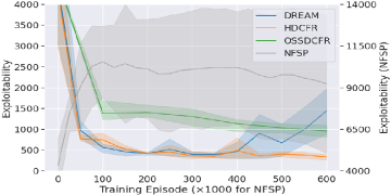
In Figure 1, we depict the learning curves of HDCFR and the baselines. Solid lines represent the mean, while shadowed areas indicate the 95% confidence intervals from repeated trials. (1) For CFR-based algorithms, the agent samples 900 trajectories, from the root to a termination state, in each training episode, and visits around 10710^{7} game states in the learning process. In contrast, the RL-based NFSP algorithm is trained over more episodes (×1000\times 1000) and the agent visits 10810^{8} game states in total during training. However, NFSP consistently underperforms in all benchmarks. Note that NFSP utilizes a separate y-axis. Evidently, NFSP is less sample efficient than the CFR-based algorithms. (2) In the absence of game models, backtracking is not allowed and so the player can sample only one action at each information set, known as outcome sampling, during game tree traversals. Thus, algorithms that require backtracking, like DCFR (Brown et al. (2019)) and DNCFR (Li et al. (2020)), cannot work directly, unless adapted with the outcome sampling scheme. It can be observed that the performance of the resulting algorithm OSSDCFR declines significantly with increasing game complexity, primarily due to the high sample variance. (3) With variance reduction techniques, DREAM achieves comparable performance to HDCFR in simpler scenarios. Yet, HDCFR, owing to its hierarchical structure, excels over DREAM in games with extended horizons, where DREAM struggles to converge. Notably, HDCFR’s superiority becomes more significant as the game complexity increases.

Further, we conducted head-to-head tournaments between HDCFR and each baseline. We select the top three checkpoints for each algorithm, resulting in total nine pairings. Each pair of strategy profiles is competed over 1,000 hands. Table 2 shows the average payoff of HDCFR’s strategy profile (Equation (18)), along with 95% confidence intervals, measured in mbb/g. A higher payoff indicates superior decision-making performance and is therefore preferred.

1/2[u1(σ1HDCFR,σ2baseline)+u2(σ1baseline,σ2HDCFR)]1/2\left[u_{1}(\sigma_{1}^{\text{HDCFR}},\sigma_{2}^{\text{baseline}})+u_{2}(\sigma_{1}^{\text{baseline}},\sigma_{2}^{\text{HDCFR}})\right] (18)

Observations from Leduc poker games in this table align with conclusions (1)-(3) previously mentioned. To further show the superiority of our algorithm, we compare its performance with baselines on larger-scale FHP games, which boast a game tree exceeding 101210^{12} in size. Due to the immense scale of FHP games, computing the best response functions is impractical, so we offer only head-to-head comparison results. Training an instance on FHP games requires roughly seven days using a device with 8 CPU cores (3rd Gen Intel Xeon) and 128 GB RAM. Our implementation leverages the RAY parallel computing framework (Moritz et al. (2018)). Still, we can see that the advantage of HDCFR grows as task difficulty goes up.

Table 2: Comparative Analysis: HDCFR vs. Baseline Algorithms in Head-to-Head Matchups
Baseline DREAM OSSDCFR NFSP
Leduc 11.94±53.79-11.94\pm 53.79 4.11±64.034.11\pm 64.03 596.55±73.46596.55\pm 73.46
Leduc_10 14.22±62.10-14.22\pm 62.10 500.0±73.22500.0\pm 73.22 642.67±109.41642.67\pm 109.41
Leduc_15 171.33±70.80171.33\pm 70.80 563.75±83.31563.75\pm 83.31 1351.5±207.271351.5\pm 207.27
Leduc_20 196.89±76.69196.89\pm 76.69 587.0±68.83587.0\pm 68.83 1725.33±206.011725.33\pm 206.01
FHP 184.58±36.75184.58\pm 36.75 68.11±36.6168.11\pm 36.61 244.61±41.36244.61\pm 41.36
FHP_10 282.42±14.20282.42\pm 14.20 343.22±15.35343.22\pm 15.35 537.39±16.91537.39\pm 16.91

4.2 Ablation Analysis

HDCFR integrates the one-step option framework (Section 2.2) and variance-reduced Monte Carlo CFR (Section 3.2 and 3.3). This section offers an ablation analysis highlighting each crucial element of our algorithm: the option framework, variance reduction, Monte Carlo sampling, and CFR.

(1) The key component of the one-step option framework is the Multi-Head Attention (MHA) mechanism which enables the agent to temporarily extend skills and so form a hierarchical policy in the learning process. Without this component in the high-level strategy (NO_MHA in Figure 2(a)), the agent struggles to converge at the final stage, akin to the behavior observed for DREAM in Figure 1(d). (2) Within HDCFR, we incorporate a baseline function to reduce variance. This function proves pivotal for extended-horizon tasks where sampling variance can escalate. Excluding the baseline function from the hierarchical strategy, as marked by NO_BASELINE in Figure 2(a), results in a substantial performance decline. (3) In Monte Carlo sampling, as outlined in Section 3.4, the traverser should use a uniformly random sampling strategy. Yet, for fair comparisons, we employ a weighted average of a uniformly random strategy (with the weight ϵ\epsilon) and the player’s current strategy (σpt\sigma^{t}_{p}). The controlling weight ϵ\epsilon is set as 0.5, aligning with configuration for the baselines. Figure 2(b) indicates that as ϵ\epsilon increases, approximately there is a correlating rise in learning performance. Notably, our design – utilizing a purely random sampling strategy at ϵ=1\epsilon=1, delivers the best result, amplifying the performance depicted in Figure 1(d). Another key aspect of Monte Carlo sampling is the number of sampled trajectories per training episode. According to Figure 2(c), increasing this count facilitates faster convergence in the initial training phase. However, it does not guarantee an improvement in the final model’s performance, and instead it would proportionally increase the overall training time. (4) As indicated by Brown et al. (2019) and Steinberger et al. (2020), slightly modifying the CFR updating rule (Equation (6)), that is, to greedily select the action with the largest regret rather than use a random one when the sum μH,μL0\mu^{H},\mu^{L}\leq 0, can speed up the convergence. We adopt the same trick and find that it can improve the convergence speed slightly, as compared to the original setting (CFR_RULE in Figure 2(a)).

Refer to caption
(a) Algorithm Design
Refer to caption
(b) Exploration Rate
Refer to caption
(c) Sample Trajectory Number
Figure 2: Learning process of different ablations on Leduc_20. (a) Without the MHA component in the high-level strategy (NO_MHA) or the baseline function for variance reduction (NO_BASELINE), convergence performance degrades significantly. Following the CFR rule (Equation (6)) results in slightly slower convergence. (b) Increased randomness in the traverser’s sample strategy enhances learning. (c) More sampled trajectories in each training episode boost initial convergence speed without affecting final performance.

4.3 Case Study: Delving into the Learned Hierarchical Strategy

Refer to caption
(a) Non-fixed
Refer to caption
(b) Fixed
Figure 3: Learning performance on Leduc_20 with transferred skills from other Leduc tasks. The transferred skills can either be fixed or not when learning a hierarchical strategy on the new scenario. The learning performance without transferred skills (labelled as HDCFR) is provided as reference. By preserving pre-learned skills, the agent focuses on mastering a high-level strategy, thus accelerating learning. However, by adjusting these skills in tandem with the high-level strategy, enhanced results are possible, as evident when using Leduc_15 skills, which peaked around episode 400.

One key benefit of hierarchical learning is the agent’s ability to use prelearned or predefined skills as foundational blocks for strategy learning, which provides a manner for integrating expert knowledge. Even in the absence of domain-specific knowledge, where rule-based skills can’t be provided as expert guidance, we can leverage skills learned from similar scenarios. Skills, functioned as policy segments, often possess greater generality than complete strategies, enabling transferred use. In Figure 3, we demonstrate the transfer of skills from various Leduc games to Leduc_20 and depict the learning outcomes. For comparison, we also present the performance without the transferred skills, labeled as HDCFR. These prelearned skills can either remain static (Figure 3(b)) or be trained with the high-level strategy (Figure 3(a)). When kept static, the agent can focus on mastering its high-level strategy to select among a set of effective skills, resulting in quicker convergence and superior end performance. Notably, the final outcomes in Figure 3(b) are intrinsically tied to the predefined skills and positively correlate with the similarity between the skills’ source task and Leduc_20. On the other hand, if the skills evolve with the high-level strategy, the improvement on the convergence speed may not be obvious, but skills can be more customized for the current task and better performance may be achieved. For instance, with Leduc_15 skills, the peak performance is reached around episode 400; with Leduc skills, training with dynamic ones (Figure 3(a)) yields better results than with static ones (Figure 3(b)). However, for Leduc_20 skills, fixed skills works better. This could be because they originate from the same task, eliminating the need for further adaptation.

Table 3: Comparison of Skill Switching Frequencies Across Different Source Tasks
Source Task Leduc Leduc_10 Leduc_15 Leduc_20
Switch Frequency 0.13630.1363 ± 4.02×10⁴\pm\ 4.02\times 10^{-4} 0.12560.1256 ± 3.43×10⁴\pm\ 3.43\times 10^{-4} 0.10880.1088 ± 2.16×10⁴\pm\ 2.16\times 10^{-4} 0.10160.1016 ± 3.64×10⁴\pm\ 3.64\times 10^{-4}

We next delve into an analysis of the learned high-level strategy. As depicted in Figure 3(b), when utilizing fixed skills from various source tasks, corresponding high-level strategies can be acquired. To determine if the high-level strategy promotes the temporal extension of skills – instead of frequently toggling between them – we employ the hierarchical strategy at each node of Leduc_20’s game tree (with 113954 nodes in total). We then calculate the frequency of skill switches in the game tree, considering all potential hands of cards and five repeated experiments. Table 3 presents the mean and 95% confidence intervals for these results. It’s evident that as the decision horizon of the skill’s source task expands, switch frequency diminishes due to prolonged single-skill durations. Notably, for Leduc_20 skills, skill switches between parent and child nodes occur only about 10% of the time. This indicates the agent’s preference for decision-making at an extended-skill level, approximately 10 steps long in average, rather than on individual actions, aligning with our anticipations.

5 Related Work

Counterfactual Regret Minimization (CFR) (Zinkevich et al. (2007)) is an algorithm for learning Nash Equilibria in extensive-form games through iterative self-play. As part of this process, it must traverse the entire game tree on every learning iteration, which is prohibitive for large-scale games. This motivates the development of Monte Carlo CFR (MCCFR) (Lanctot et al. (2009)), which samples trajectories traversing part of the tree to allow for significantly faster iterations. Yet, the variance of Monte Carlo outcome sampling could be an issue, especially for long sample trajectories. The authors of (Schmid et al. (2019); Davis et al. (2020)) then propose to introduce baseline functions for variance reduction. Notably, all methods mentioned above are tabular-based. For games with large state space, domain-specific abstraction schemes (Ganzfried and Sandholm (2014b); Moravčík et al. (2017)) are required to shrink them to a manageable size by clustering states into buckets, which necessitates expert knowledge and is not applicable to all games.

To obviate the need of abstractions, several CFR variants with function approximators have emerged. Pioneering this was Regression CFR (Waugh et al. (2015)), which adopts regression trees to model cumulative regrets but relies on hand-crafted features and full traversals of the game tree. Subsequently, several works (Brown et al. (2019); Li et al. (2020); Steinberger (2019); Li et al. (2021b)) propose to model the cumulative counterfactual regrets and average strategies in MCCFR as neural networks to enhance the scalability. However, all these methods rely on knowledge of the game model to realize backtracking (i.e., sampling multiple actions at an information set) for regret estimation. As a model-free approach, Neural Fictitious Self-Play (NFSP) (Heinrich and Silver (2016)) is the first deep reinforcement learning algorithm to learn a Nash Equilibrium in two-player imperfect information games through self-play. Since its advent, various policy gradient and actor-critic methods have been shown to have similar convergence properties if tuned appropriately (Lanctot et al. (2017); Srinivasan et al. (2018)). However, fictitious play empirically converges slower than CFR-based approaches in many settings. DREAM (Steinberger et al. (2020)) extends DCFR with variance-reduction techniques from Davis et al. (2020) and represents the state-of-the-art in model-free algorithms of this area. Compared with DREAM, our algorithm enables hierarchical learning with (prelearned) skills and empirically show enhanced performance on longer-horizon games.

As another important module of HDCFR, the option framework (Sutton et al. (1999)) enables learning and planning at multiple temporal levels and has been widely adopted in reinforcement learning. Multiple research areas centered on this framework have been developed. Unsupervised Option Discovery aims at discovering skills that are diverse and efficient for downstream task learning without supervision from reward signals, for which algorithms have been proposed for both single-agent (Eysenbach et al. (2019); Jinnai et al. (2020); Chen et al. (2022a)) and collaborative multi-agent scenarios (Chen et al. (2022c, b); Zhang et al. (2022)). Hierarchical Reinforcement Learning (Zhang and Whiteson (2019); Li et al. (2021a)) and Hierarchical Imitation Learning (Jing et al. (2021); Chen et al. (2023a, b)), on the other hand, aim at directly learning a hierarchical policy incorporated with skills, either from interactions with the environment or expert demonstrations. As a pioneering effort to amalgamate options with CFR, HDCFR not only offers a robust theoretical foundation but also demonstrates resilient empirical performance against leading algorithms in zero-sum imperfect-information games.

6 Conclusion

In this research, we present the first hierarchical version of Counterfactual Regret Minimization (CFR) by utilizing the option framework. Initially, we establish its theoretical foundations in a tabular setting, introducing Hierarchical CFR updating rules that are guaranteed to converge. Then, we provide a low-variance Monte Carlo sampling extension for scalable learning in tasks without perfect game models or encompassing deep game trees. Further, we incorporate neural networks as function approximators, devising deep learning objectives that align with the theoretical outcomes in the tabular setting, thereby empowering our HDCFR algorithm to manage vast state spaces. Evaluations in complex two-player zero-sum games show HDCFR’s superiority over leading algorithms in this field and its advantage becomes more significant as the decision horizon increases, underscoring HDCFR’s great potential in tasks involving deep game trees. Moreover, we show empirically that the learned high-level strategy can temporarily extend skills to utilize the hierarchical subtask structures in long-horizon tasks, and the learned skills can be transferred to different tasks, serving as expert knowledge injections to facilitate learning. Finally, our algorithm provides a novel framework to learn with predefined skills in zero-sum IIGs. An interesting future research direction could be interactive learning with human inputs as skills.

References

  • Abernethy et al. (2011) J. Abernethy, P. L. Bartlett, and E. Hazan. Blackwell approachability and no-regret learning are equivalent. In Proceedings of the 24th Annual Conference on Learning Theory, pages 27–46. JMLR Workshop and Conference Proceedings, 2011.
  • Bakhtin et al. (2022) A. Bakhtin, N. Brown, E. Dinan, G. Farina, C. Flaherty, D. Fried, A. Goff, J. Gray, H. Hu, A. P. Jacob, M. Komeili, K. Konath, M. Kwon, A. Lerer, M. Lewis, A. H. Miller, S. Mitts, A. Renduchintala, S. Roller, D. Rowe, W. Shi, J. Spisak, A. Wei, D. Wu, H. Zhang, and M. Zijlstra. Human-level play in the game of diplomacy by combining language models with strategic reasoning. Science, pages 1067–1074, 2022.
  • Bowling et al. (2015) M. Bowling, N. Burch, M. Johanson, and O. Tammelin. Heads-up limit hold’em poker is solved. Science, 347(6218):145–149, 2015.
  • Brown and Sandholm (2017) N. Brown and T. Sandholm. Safe and nested subgame solving for imperfect-information games. In Proceedings of the 31st Annual Conference on Neural Information Processing Systems, pages 689–699, 2017.
  • Brown and Sandholm (2018) N. Brown and T. Sandholm. Superhuman ai for heads-up no-limit poker: Libratus beats top professionals. Science, 359(6374):418–424, 2018.
  • Brown et al. (2018) N. Brown, T. Sandholm, and B. Amos. Depth-limited solving for imperfect-information games. In Proceedings of the 32nd Annual Conference on Neural Information Processing Systems, pages 7674–7685, 2018.
  • Brown et al. (2019) N. Brown, A. Lerer, S. Gross, and T. Sandholm. Deep counterfactual regret minimization. In Proceedings of the 36th International Conference on Machine Learning, volume 97 of Proceedings of Machine Learning Research, pages 793–802. PMLR, 2019.
  • Chen et al. (2022a) J. Chen, V. Aggarwal, and T. Lan. ODPP: A unified algorithm framework for unsupervised option discovery based on determinantal point process. CoRR, abs/2212.00211, 2022a.
  • Chen et al. (2022b) J. Chen, J. Chen, T. Lan, and V. Aggarwal. Learning multi-agent options for tabular reinforcement learning using factor graphs. IEEE Transactions on Artificial Intelligence, pages 1–13, 2022b. doi: 10.1109/tai.2022.3195818.
  • Chen et al. (2022c) J. Chen, J. Chen, T. Lan, and V. Aggarwal. Multi-agent covering option discovery based on kronecker product of factor graphs. IEEE Transactions on Artificial Intelligence, 2022c.
  • Chen et al. (2023a) J. Chen, T. Lan, and V. Aggarwal. Option-aware adversarial inverse reinforcement learning for robotic control. In 2023 IEEE International Conference on Robotics and Automation (ICRA), pages 5902–5908. IEEE, 2023a.
  • Chen et al. (2023b) J. Chen, D. Tamboli, T. Lan, and V. Aggarwal. Multi-task hierarchical adversarial inverse reinforcement learning. In Proceedings of the 40th International Conference on Machine Learning, volume 202 of Proceedings of Machine Learning Research, pages 4895–4920. PMLR, 2023b.
  • Davis et al. (2020) T. Davis, M. Schmid, and M. Bowling. Low-variance and zero-variance baselines for extensive-form games. In Proceedings of the 37th International Conference on Machine Learning, volume 119 of Proceedings of Machine Learning Research, pages 2392–2401. PMLR, 2020.
  • Eysenbach et al. (2019) B. Eysenbach, A. Gupta, J. Ibarz, and S. Levine. Diversity is all you need: Learning skills without a reward function. In Proceedings of the 7th International Conference on Learning Representations. OpenReview.net, 2019.
  • Fu et al. (2022) H. Fu, W. Liu, S. Wu, Y. Wang, T. Yang, K. Li, J. Xing, B. Li, B. Ma, Q. Fu, and W. Yang. Actor-critic policy optimization in a large-scale imperfect-information game. In Proceedings of the 10th International Conference on Learning Representations. OpenReview.net, 2022.
  • Ganzfried and Sandholm (2014a) S. Ganzfried and T. Sandholm. Potential-aware imperfect-recall abstraction with earth mover’s distance in imperfect-information games. In Proceedings of the 28th AAAI Conference on Artificial Intelligence, pages 682–690. AAAI Press, 2014a.
  • Ganzfried and Sandholm (2014b) S. Ganzfried and T. Sandholm. Potential-aware imperfect-recall abstraction with earth mover’s distance in imperfect-information games. In Proceedings of 28th the AAAI Conference on Artificial Intelligence, volume 28, 2014b.
  • Gibson et al. (2012) R. G. Gibson, M. Lanctot, N. Burch, D. Szafron, and M. Bowling. Generalized sampling and variance in counterfactual regret minimization. In Proceedings of the 26th AAAI Conference on Artificial Intelligence. AAAI Press, 2012.
  • Heinrich and Silver (2016) J. Heinrich and D. Silver. Deep reinforcement learning from self-play in imperfect-information games. CoRR, abs/1603.01121, 2016.
  • Jing et al. (2021) M. Jing, W. Huang, F. Sun, X. Ma, T. Kong, C. Gan, and L. Li. Adversarial option-aware hierarchical imitation learning. In Proceedings of the 38th International Conference on Machine Learning, pages 5097–5106. PMLR, 2021.
  • Jinnai et al. (2020) Y. Jinnai, J. W. Park, M. C. Machado, and G. D. Konidaris. Exploration in reinforcement learning with deep covering options. In Proceedings of the 8th International Conference on Learning Representations. OpenReview.net, 2020.
  • Kakkad et al. (2019) V. Kakkad, H. Shah, R. Patel, and N. Doshi. A comparative study of applications of game theory in cyber security and cloud computing. Procedia Computer Science, 155:680–685, 2019.
  • Lanctot et al. (2009) M. Lanctot, K. Waugh, M. Zinkevich, and M. H. Bowling. Monte carlo sampling for regret minimization in extensive games. In Proceedings of the 23rd Annual Conference on Neural Information Processing Systems, pages 1078–1086. Curran Associates, Inc., 2009.
  • Lanctot et al. (2017) M. Lanctot, V. F. Zambaldi, A. Gruslys, A. Lazaridou, K. Tuyls, J. Pérolat, D. Silver, and T. Graepel. A unified game-theoretic approach to multiagent reinforcement learning. In Advances in Neural Information Processing Systems 30, pages 4190–4203, 2017.
  • Li et al. (2021a) C. Li, D. Song, and D. Tao. The skill-action architecture: Learning abstract action embeddings for reinforcement learning. In Submissions of the 9th International Conference on Learning Representations, 2021a.
  • Li et al. (2020) H. Li, K. Hu, S. Zhang, Y. Qi, and L. Song. Double neural counterfactual regret minimization. In Proceedings of the 8th International Conference on Learning Representations. OpenReview.net, 2020.
  • Li et al. (2021b) H. Li, X. Wang, Z. Guo, J. Zhang, and S. Qi. D2cfr: Minimize counterfactual regret with deep dueling neural network. arXiv preprint arXiv:2105.12328, 2021b.
  • Moravcik et al. (2016) M. Moravcik, M. Schmid, K. Ha, M. Hladík, and S. J. Gaukrodger. Refining subgames in large imperfect information games. In Proceedings of the 30th AAAI Conference on Artificial Intelligence, pages 572–578. AAAI Press, 2016.
  • Moravčík et al. (2017) M. Moravčík, M. Schmid, N. Burch, V. Lisỳ, D. Morrill, N. Bard, T. Davis, K. Waugh, M. Johanson, and M. Bowling. Deepstack: Expert-level artificial intelligence in heads-up no-limit poker. Science, 356(6337):508–513, 2017.
  • Moritz et al. (2018) P. Moritz, R. Nishihara, S. Wang, A. Tumanov, R. Liaw, E. Liang, M. Elibol, Z. Yang, W. Paul, M. I. Jordan, and I. Stoica. Ray: A distributed framework for emerging AI applications. In 13th USENIX Symposium on Operating Systems Design and Implementation, pages 561–577. USENIX Association, 2018.
  • Noe et al. (2012) T. H. Noe, M. Rebello, and J. Wang. Learning to bid: The design of auctions under uncertainty and adaptation. Games and Economic Behavior, pages 620–636, 2012.
  • Osborne and Rubinstein (1994) M. J. Osborne and A. Rubinstein. A course in game theory. MIT press, 1994.
  • Sandholm (2015) T. Sandholm. Abstraction for solving large incomplete-information games. In Proceedings of the 29th AAAI Conference on Artificial Intelligence, pages 4127–4131. AAAI Press, 2015.
  • Schmid et al. (2019) M. Schmid, N. Burch, M. Lanctot, M. Moravcik, R. Kadlec, and M. Bowling. Variance reduction in monte carlo counterfactual regret minimization (VR-MCCFR) for extensive form games using baselines. In Proceedings of 33rd the AAAI Conference on Artificial Intelligence, pages 2157–2164. AAAI Press, 2019.
  • Southey et al. (2005) F. Southey, M. H. Bowling, B. Larson, C. Piccione, N. Burch, D. Billings, and D. C. Rayner. Bayes’ bluff: Opponent modelling in poker. In Proceedings of the 21st Conference in Uncertainty in Artificial Intelligence, pages 550–558, 2005.
  • Srinivasan et al. (2018) S. Srinivasan, M. Lanctot, V. F. Zambaldi, J. Pérolat, K. Tuyls, R. Munos, and M. Bowling. Actor-critic policy optimization in partially observable multiagent environments. In Proceedings of the 32nd Annual Conference on Neural Information Processing Systems, pages 3426–3439, 2018.
  • Steinberger (2019) E. Steinberger. Single deep counterfactual regret minimization. CoRR, abs/1901.07621, 2019.
  • Steinberger (2020) E. Steinberger. Pokerrl. https://github.com/EricSteinberger/DREAM, 2020.
  • Steinberger et al. (2020) E. Steinberger, A. Lerer, and N. Brown. DREAM: deep regret minimization with advantage baselines and model-free learning. CoRR, abs/2006.10410, 2020.
  • Sutton et al. (1999) R. S. Sutton, D. Precup, and S. Singh. Between mdps and semi-mdps: A framework for temporal abstraction in reinforcement learning. Artificial Intelligence, 112(1):181–211, 1999. ISSN 0004-3702. doi: https://doi.org/10.1016/S0004-3702(99)00052-1.
  • Vaswani et al. (2017) A. Vaswani, N. Shazeer, N. Parmar, J. Uszkoreit, L. Jones, A. N. Gomez, L. Kaiser, and I. Polosukhin. Attention is all you need. In Proceedings of the 31st Annual Conference on Neural Information Processing Systems, pages 5998–6008, 2017.
  • Waugh et al. (2015) K. Waugh, D. Morrill, J. A. Bagnell, and M. H. Bowling. Solving games with functional regret estimation. In Proceedings of the 29th AAAI Conference on Artificial Intelligence, pages 2138–2145. AAAI Press, 2015.
  • Zhang et al. (2022) F. Zhang, C. Jia, Y.-C. Li, L. Yuan, Y. Yu, and Z. Zhang. Discovering generalizable multi-agent coordination skills from multi-task offline data. In Proceedings of the 11th International Conference on Learning Representations, 2022.
  • Zhang and Whiteson (2019) S. Zhang and S. Whiteson. DAC: the double actor-critic architecture for learning options. In Proceedings of the 33rd Annual Conference on Neural Information Processing Systems, pages 2010–2020, 2019.
  • Zinkevich et al. (2007) M. Zinkevich, M. Johanson, M. H. Bowling, and C. Piccione. Regret minimization in games with incomplete information. In Proceedings of the 21st Annual Conference on Neural Information Processing Systems, pages 1729–1736. Curran Associates, Inc., 2007.

Appendix A Proof of Theorem 2

Define D(I)D(I) to be the information sets of player ii reachable from II (including II), and σ|D(I)σi\sigma|_{D(I)\rightarrow\sigma^{{}^{\prime}}_{i}} to be a strategy profile equal to σ\sigma except that player ii adopts σi\sigma^{{}^{\prime}}_{i} in the information sets contained in D(I)D(I). Then, the average overall regret starting from II (IiI\in\mathcal{I}_{i}) can be defined as:

Rfull,iT(I)=1Tmaxσit=1Tπiσt(I)(ui(σt|D(I)σi,I)ui(σt,I))\displaystyle R_{full,i}^{T}(I)=\frac{1}{T}\max_{\sigma^{{}^{\prime}}_{i}}\sum_{t=1}^{T}\pi^{\sigma^{t}}_{-i}(I)(u_{i}(\sigma^{t}|_{D(I)\rightarrow\sigma^{{}^{\prime}}_{i}},I)-u_{i}(\sigma^{t},I)) (19)

Further, we define Si(I,a~)S_{i}(I,\widetilde{a}) to be the set of all possible next information sets of player ii given that action a~A~(I)\widetilde{a}\in\widetilde{A}(I) was just selected at II and define Si(I)=a~A~(I)Si(I,a~)S_{i}(I)=\bigcup_{\widetilde{a}\in\widetilde{A}(I)}S_{i}(I,\widetilde{a}), Si(Iz)=aA(I)Si(I,za)S_{i}(Iz)=\bigcup_{a\in A(I)}S_{i}(I,za). Then, we have the following lemma:

Lemma 1

Rfull,iT,+(I)Ri,+T,H(I)+zZ(I)Ri,+T,L(I,z)+ISi(I)Rfull,iT,+(I)R_{full,i}^{T,+}(I)\leq R_{i,+}^{T,H}(I)+\sum_{z\in Z(I)}R^{T,L}_{i,+}(I,z)+\sum_{I^{\prime}\in S_{i}(I)}R_{full,i}^{T,+}(I^{\prime})

Proof 

Rfull,iT(I)=1Tmaxσit=1Tπiσt(I)(ui(σt|D(I)σi,I)ui(σt,I))\displaystyle R_{full,i}^{T}(I)=\frac{1}{T}\max_{\sigma^{{}^{\prime}}_{i}}\sum_{t=1}^{T}\pi^{\sigma^{t}}_{-i}(I)(u_{i}(\sigma^{t}|_{D(I)\rightarrow\sigma^{{}^{\prime}}_{i}},I)-u_{i}(\sigma^{t},I)) (20)
=1TmaxzZ(I)maxσit=1Tπiσt(I)[(ui(σt|Iz,I)ui(σt,I))+(ui(σt|D(Iz)σi,Iz)ui(σt,Iz))]\displaystyle=\frac{1}{T}\max_{z\in Z(I)}\max_{\sigma^{{}^{\prime}}_{i}}\sum_{t=1}^{T}\pi^{\sigma^{t}}_{-i}(I)\left[(u_{i}(\sigma^{t}|_{I\rightarrow z},I)-u_{i}(\sigma^{t},I))+(u_{i}(\sigma^{t}|_{D(Iz)\rightarrow\sigma^{{}^{\prime}}_{i}},Iz)-u_{i}(\sigma^{t},Iz))\right]
1TmaxzZ(I)t=1Tπiσt(I)(ui(σt|Iz,I)ui(σt,I))+\displaystyle\leq\frac{1}{T}\max_{z\in Z(I)}\sum_{t=1}^{T}\pi^{\sigma^{t}}_{-i}(I)(u_{i}(\sigma^{t}|_{I\rightarrow z},I)-u_{i}(\sigma^{t},I))+
1TmaxzZ(I)maxσit=1Tπiσt(I)(ui(σt|D(Iz)σi,Iz)ui(σt,Iz))\displaystyle\ \ \ \ \ \frac{1}{T}\max_{z\in Z(I)}\max_{\sigma^{{}^{\prime}}_{i}}\sum_{t=1}^{T}\pi^{\sigma^{t}}_{-i}(I)(u_{i}(\sigma^{t}|_{D(Iz)\rightarrow\sigma^{{}^{\prime}}_{i}},Iz)-u_{i}(\sigma^{t},Iz))
=RiT,H(I)+1TmaxzZ(I)maxσit=1Tπiσt(Iz)(ui(σt|D(Iz)σi,Iz)ui(σt,Iz))\displaystyle=R_{i}^{T,H}(I)+\frac{1}{T}\max_{z\in Z(I)}\max_{\sigma^{{}^{\prime}}_{i}}\sum_{t=1}^{T}\pi^{\sigma^{t}}_{-i}(Iz)(u_{i}(\sigma^{t}|_{D(Iz)\rightarrow\sigma^{{}^{\prime}}_{i}},Iz)-u_{i}(\sigma^{t},Iz))
RiT,H(I)+zZ(I)[1Tmaxσit=1Tπiσt(Iz)(ui(σt|D(Iz)σi,Iz)ui(σt,Iz))]+\displaystyle\leq R_{i}^{T,H}(I)+\sum_{z\in Z(I)}\left[\frac{1}{T}\max_{\sigma^{{}^{\prime}}_{i}}\sum_{t=1}^{T}\pi^{\sigma^{t}}_{-i}(Iz)(u_{i}(\sigma^{t}|_{D(Iz)\rightarrow\sigma^{{}^{\prime}}_{i}},Iz)-u_{i}(\sigma^{t},Iz))\right]^{+}
=RiT,H(I)+zZ(I)Rfull,iT,+(Iz)\displaystyle=R_{i}^{T,H}(I)+\sum_{z\in Z(I)}R_{full,i}^{T,+}(Iz)
Rfull,iT(Iz)=1Tmaxσit=1Tπiσt(Iz)(ui(σt|D(Iz)σi,Iz)ui(σt,Iz))\displaystyle R_{full,i}^{T}(Iz)=\frac{1}{T}\max_{\sigma^{{}^{\prime}}_{i}}\sum_{t=1}^{T}\pi^{\sigma^{t}}_{-i}(Iz)(u_{i}(\sigma^{t}|_{D(Iz)\rightarrow\sigma^{{}^{\prime}}_{i}},Iz)-u_{i}(\sigma^{t},Iz)) (21)
=1TmaxaA(I)maxσit=1Tπiσt(Iz)[(ui(σt|Iza,Iz)ui(σt,Iz))+\displaystyle=\frac{1}{T}\max_{a\in A(I)}\max_{\sigma^{{}^{\prime}}_{i}}\sum_{t=1}^{T}\pi^{\sigma^{t}}_{-i}(Iz)[(u_{i}(\sigma^{t}|_{Iz\rightarrow a},Iz)-u_{i}(\sigma^{t},Iz))+
ISi(I,za)Pσit(I|I,za)(ui(σt|D(I)σi,I)ui(σt,I))]\displaystyle\qquad\qquad\qquad\qquad\qquad\qquad\quad\sum_{I^{\prime}\in S_{i}(I,za)}P_{\sigma^{t}_{-i}}(I^{\prime}|I,za)(u_{i}(\sigma^{t}|_{D(I^{\prime})\rightarrow\sigma^{{}^{\prime}}_{i}},I^{\prime})-u_{i}(\sigma^{t},I^{\prime}))]
=RiT,L(I,z)+maxaA(I)ISi(I,za)1Tmaxσit=1Tπiσt(I)(ui(σt|D(I)σi,I)ui(σt,I))\displaystyle=R_{i}^{T,L}(I,z)+\max_{a\in A(I)}\sum_{I^{\prime}\in S_{i}(I,za)}\frac{1}{T}\max_{\sigma^{{}^{\prime}}_{i}}\sum_{t=1}^{T}\pi^{\sigma^{t}}_{-i}(I^{\prime})(u_{i}(\sigma^{t}|_{D(I^{\prime})\rightarrow\sigma^{{}^{\prime}}_{i}},I^{\prime})-u_{i}(\sigma^{t},I^{\prime}))
=RiT,L(I,z)+maxaA(I)ISi(I,za)Rfull,iT(I)\displaystyle=R_{i}^{T,L}(I,z)+\max_{a\in A(I)}\sum_{I^{\prime}\in S_{i}(I,za)}R_{full,i}^{T}(I^{\prime})
RiT,L(I,z)+ISi(Iz)Rfull,iT,+(I)\displaystyle\leq R_{i}^{T,L}(I,z)+\sum_{I^{\prime}\in S_{i}(Iz)}R_{full,i}^{T,+}(I^{\prime})

In Equation (20) and (21), we employ the one-step look-ahead expansion (Equation (10) in Zinkevich et al. (2007)) for the second line. At iteration tt, when player ii selects a hierarchical action a~=(za)\widetilde{a}=(za), it will transit to the subsequent information set ISi(I,za)I^{\prime}\in S_{i}(I,za) with a probability of Pσit(I|I,za)P_{\sigma^{t}_{-i}}(I^{\prime}|I,za), since only player i-i will act between II and II^{\prime} according to σit\sigma^{t}_{-i}. According to the definition of the reach probability, πi(Iz)=πi(I)\pi_{-i}(Iz)=\pi_{-i}(I) (since zz and aa are executed by player ii) and πi(I)Pσit(I|I,za)=πi(I)\pi_{-i}(I)P_{\sigma^{t}_{-i}}(I^{\prime}|I,za)=\pi_{-i}(I^{\prime}). Combining Equation (20) and (21), we can get:

Rfull,iT(I)RiT,H(I)+zZ(I)Rfull,iT,+(Iz)\displaystyle R_{full,i}^{T}(I)\leq R_{i}^{T,H}(I)+\sum_{z\in Z(I)}R_{full,i}^{T,+}(Iz) (22)
RiT,H(I)+zZ(I)[Ri,+T,L(I,z)+ISi(Iz)Rfull,iT,+(I)]\displaystyle\leq R_{i}^{T,H}(I)+\sum_{z\in Z(I)}\left[R_{i,+}^{T,L}(I,z)+\sum_{I^{\prime}\in S_{i}(Iz)}R_{full,i}^{T,+}(I^{\prime})\right]
=RiT,H(I)+zZ(I)Ri,+T,L(I,z)+zZ(I)ISi(Iz)Rfull,iT,+(I)\displaystyle=R_{i}^{T,H}(I)+\sum_{z\in Z(I)}R_{i,+}^{T,L}(I,z)+\sum_{z\in Z(I)}\sum_{I^{\prime}\in S_{i}(Iz)}R_{full,i}^{T,+}(I^{\prime})
=RiT,H(I)+zZ(I)Ri,+T,L(I,z)+ISi(I)Rfull,iT,+(I)\displaystyle=R_{i}^{T,H}(I)+\sum_{z\in Z(I)}R_{i,+}^{T,L}(I,z)+\sum_{I^{\prime}\in S_{i}(I)}R_{full,i}^{T,+}(I^{\prime})

In previous derivations, we have repeatedly employed the inequality max(a+b,0)max(a,0)+max(b,0)\max(a+b,0)\leq\max(a,0)+\max(b,0), which holds for all a,ba,b\in\mathbb{R}, as in the last inequality of Equation (20) and (21). By applying this inequality once more to Equation (22), we can obtain Lemma 1.  

Lemma 2

Rfull,iT,+(I)ID(I)[Ri,+T,H(I)+zZ(I)Ri,+T,L(I,z)]R_{full,i}^{T,+}(I)\leq\sum_{I^{\prime}\in D(I)}\left[R_{i,+}^{T,H}(I^{\prime})+\sum_{z\in Z(I^{\prime})}R_{i,+}^{T,L}(I^{\prime},z)\right]

Proof  We prove this lemma by induction on the height of the information set II on the game tree. When the height is 1, i.e., Si(I)=S_{i}(I)=\emptyset, D(I)={I}D(I)=\{I\}, then Lemma 1 implies Lemma 2. Now, for the general case:

Rfull,iT,+(I)Ri,+T,H(I)+zZ(I)Ri,+T,L(I,z)+ISi(I)Rfull,iT,+(I)\displaystyle R_{full,i}^{T,+}(I)\leq R_{i,+}^{T,H}(I)+\sum_{z\in Z(I)}R^{T,L}_{i,+}(I,z)+\sum_{I^{\prime}\in S_{i}(I)}R_{full,i}^{T,+}(I^{\prime}) (23)
Ri,+T,H(I)+zZ(I)Ri,+T,L(I,z)+ISi(I)I′′D(I)[Ri,+T,H(I′′)+zZ(I′′)Ri,+T,L(I′′,z)]\displaystyle\leq R_{i,+}^{T,H}(I)+\sum_{z\in Z(I)}R^{T,L}_{i,+}(I,z)+\sum_{I^{\prime}\in S_{i}(I)}\sum_{I^{\prime\prime}\in D(I^{\prime})}\left[R_{i,+}^{T,H}(I^{\prime\prime})+\sum_{z\in Z(I^{\prime\prime})}R_{i,+}^{T,L}(I^{\prime\prime},z)\right]
=ID(I)[Ri,+T,H(I)+zZ(I)Ri,+T,L(I,z)]\displaystyle=\sum_{I^{\prime}\in D(I)}\left[R_{i,+}^{T,H}(I^{\prime})+\sum_{z\in Z(I^{\prime})}R_{i,+}^{T,L}(I^{\prime},z)\right]

In the second line, we employ the induction hypothesis. In the third line, we use the following facts: D(I)={I}ISi(I)D(I)D(I)=\{I\}\cup\bigcup_{I^{\prime}\in S_{i}(I)}D(I^{\prime}), {I}ISi(I)D(I)=\{I\}\cap\bigcup_{I^{\prime}\in S_{i}(I)}D(I^{\prime})=\emptyset, and D(I)D(I′′)=D(I^{\prime})\cap D(I^{\prime\prime})=\emptyset for all distinct I,I′′Si(I)I^{\prime},I^{\prime\prime}\in S_{i}(I). The third fact here is derived from the perfect recall property of the game: all players can recall their previous (hierarchical) actions and the corresponding information sets. Then, D(I)D(I′′)=D(I^{\prime})\cap D(I^{\prime\prime})=\emptyset because elements from the two sets possess distinct prefixes (i.e., II^{\prime} and I′′I^{\prime\prime}).  
Last, for the average overall regret, we have Rfull,iT=Rfull,iT()R_{full,i}^{T}=R_{full,i}^{T}(\emptyset), where \emptyset corresponds to the start of the game tree and D()=iD(\emptyset)=\mathcal{I}_{i}. Applying Lemma 2, we can get the theorem: Rfull,iTRfull,iT,+()Ii[Ri,+T,H(I)+zZ(I)Ri,+T,L(I,z)]R_{full,i}^{T}\leq R_{full,i}^{T,+}(\emptyset)\leq\sum_{I\in\mathcal{I}_{i}}\left[R_{i,+}^{T,H}(I)+\sum_{z\in Z(I)}R_{i,+}^{T,L}(I,z)\right].

Appendix B Proof of Theorem 3

Regret matching can be defined in a domain where a fixed set of actions AA and a payoff function ut:Au^{t}:A\rightarrow\mathbb{R} exist. At each iteration tt, a distribution over the actions, σt\sigma^{t}, is chosen based on the cumulative regret Rt:AR^{t}:A\rightarrow\mathbb{R}. Specifically, the cumulative regret at iteration TT for not playing action aa is defined as:

RT(a)=1Tt=1T[ut(a)aAσt(a)ut(a)]\displaystyle R^{T}(a)=\frac{1}{T}\sum_{t=1}^{T}\left[u^{t}(a)-\sum_{a^{\prime}\in A}\sigma^{t}(a^{\prime})u^{t}(a^{\prime})\right] (24)

where σt(a)\sigma^{t}(a) is obtained by:

σt(a)={Rt1,+(a)/μ,μ>0,1/|A|,o\w.μ=aARt1,+(a)\displaystyle\sigma^{t}(a)=\left\{\begin{aligned} R^{t-1,+}(a)/\mu&,&\mu>0,\\ 1/|A|&,&o\backslash w.\end{aligned}\right.\ \ \ \ \mu=\sum_{a^{\prime}\in A}R^{t-1,+}(a^{\prime}) (25)

Then, we have the following lemma (Theorem 8 in Zinkevich et al. (2007)):

Lemma 3

maxaART(a)Δu|A|T\max_{a\in A}R^{T}(a)\leq\frac{\Delta_{u}\sqrt{|A|}}{\sqrt{T}}, where Δu=maxt{1,,T}maxa,aA(ut(a)ut(a))\Delta_{u}=\max_{t\in\{1,\cdots,T\}}\max_{a,a^{\prime}\in A}(u^{t}(a)-u^{t}(a^{\prime})).

To apply this lemma, we must transform the definitions of RiT,HR_{i}^{T,H} and RiT,LR_{i}^{T,L} in Equation (5) to a form resembling Equation (24). With Equation (5) and (2), we can get:

RiT,H(z|I)\displaystyle R^{T,H}_{i}(z|I) =1Tt=1T[hIπiσt(h)hHTSui(h)πσt(hz,h)\displaystyle=\frac{1}{T}\sum_{t=1}^{T}[\sum_{h\in I}\pi_{-i}^{\sigma^{t}}(h)\sum_{h^{\prime}\in H_{TS}}u_{i}(h^{\prime})\pi^{\sigma^{t}}(hz,h^{\prime})- (26)
hIπiσt(h)hHTSui(h)zZ(h)σtH(z|h)πσt(hz,h)]\displaystyle\qquad\quad\ \ \ \ \sum_{h\in I}\pi_{-i}^{\sigma^{t}}(h)\sum_{h^{\prime}\in H_{TS}}u_{i}(h^{\prime})\sum_{z^{\prime}\in Z(h)}\sigma^{H}_{t}(z^{\prime}|h)\pi^{\sigma^{t}}(hz^{\prime},h^{\prime})]
=1Tt=1T[hIπiσt(h)hHTSui(h)πσt(hz,h)\displaystyle=\frac{1}{T}\sum_{t=1}^{T}[\sum_{h\in I}\pi_{-i}^{\sigma^{t}}(h)\sum_{h^{\prime}\in H_{TS}}u_{i}(h^{\prime})\pi^{\sigma^{t}}(hz,h^{\prime})-
zZ(I)σtH(z|I)hIπiσt(h)hHTSui(h)πσt(hz,h)]\displaystyle\qquad\ \ \ \ \ \sum_{z^{\prime}\in Z(I)}\sigma^{H}_{t}(z^{\prime}|I)\sum_{h\in I}\pi_{-i}^{\sigma^{t}}(h)\sum_{h^{\prime}\in H_{TS}}u_{i}(h^{\prime})\pi^{\sigma^{t}}(hz^{\prime},h^{\prime})]
=1Tt=1T[vtH(z)zZ(I)σtH(z|I)vtH(z)]\displaystyle=\frac{1}{T}\sum_{t=1}^{T}\left[v_{t}^{H}(z)-\sum_{z^{\prime}\in Z(I)}\sigma^{H}_{t}(z^{\prime}|I)v_{t}^{H}(z^{\prime})\right]

Applying the same process on RiT,L(a|I,z)R_{i}^{T,L}(a|I,z), we can get:

RiT,L(a|I,z)=1Tt=1T[vtL(a)aA(I)σtL(a|I,z)vtL(a)]\displaystyle R^{T,L}_{i}(a|I,z)=\frac{1}{T}\sum_{t=1}^{T}\left[v_{t}^{L}(a)-\sum_{a^{\prime}\in A(I)}\sigma^{L}_{t}(a^{\prime}|I,z)v_{t}^{L}(a^{\prime})\right] (27)
vtL(a)=hIπiσt(h)hHTSui(h)πσt(hza,h)\displaystyle\qquad\ \ v_{t}^{L}(a)=\sum_{h\in I}\pi_{-i}^{\sigma^{t}}(h)\sum_{h^{\prime}\in H_{TS}}u_{i}(h^{\prime})\pi^{\sigma^{t}}(hza,h^{\prime})

Then, we can apply Lemma 3 and obtain:

maxzZ(I)RiT,H(z|I)=RiT,H(I)ΔvH|Z(I)|TΔu,i|Z(I)|T\displaystyle\ \ \ \max_{z\in Z(I)}R^{T,H}_{i}(z|I)=R^{T,H}_{i}(I)\leq\frac{\Delta_{v^{H}}\sqrt{|Z(I)|}}{\sqrt{T}}\leq\frac{\Delta_{u,i}\sqrt{|Z(I)|}}{\sqrt{T}} (28)
maxaA(I)RiT,L(a|I,z)=RiT,L(I,z)ΔvL|A(I)|TΔu,i|A(I)|T\displaystyle\max_{a\in A(I)}R^{T,L}_{i}(a|I,z)=R^{T,L}_{i}(I,z)\leq\frac{\Delta_{v^{L}}\sqrt{|A(I)|}}{\sqrt{T}}\leq\frac{\Delta_{u,i}\sqrt{|A(I)|}}{\sqrt{T}}

Here, Δu,i=maxhHTSui(h)minhHTSui(h)\Delta_{u,i}=\max_{h^{\prime}\in H_{TS}}u_{i}(h^{\prime})-\min_{h^{\prime}\in H_{TS}}u_{i}(h^{\prime}) is the range of the payoff function for ii, which covers ΔvH\Delta_{v^{H}} and ΔvL\Delta_{v^{L}}. We can directly apply Lemma 3, because the regret matching is adopted at each information set independently as defined in Equation (6). By integrating Equation 28 and Theorem 2, we then get:

Rfull,iT\displaystyle R_{full,i}^{T} Ii[Δu,i|Z(I)|T+zZ(I)Δu,i|A(I)|T]\displaystyle\leq\sum_{I\in\mathcal{I}_{i}}\left[\frac{\Delta_{u,i}\sqrt{|Z(I)|}}{\sqrt{T}}+\sum_{z\in Z(I)}\frac{\Delta_{u,i}\sqrt{|A(I)|}}{\sqrt{T}}\right] (29)
Δu,i|i|T(|Zi|+|Zi||Ai|)\displaystyle\leq\frac{\Delta_{u,i}|\mathcal{I}_{i}|}{\sqrt{T}}(\sqrt{|Z_{i}|}+|Z_{i}|\sqrt{|A_{i}|})

where |i||\mathcal{I}_{i}| is the number of information sets for player ii, |Ai|=maxh:P(h)=i|A(h)||A_{i}|=\max_{h:P(h)=i}|A(h)|, |Zi|=maxh:P(h)=i|Z(h)||Z_{i}|=\max_{h:P(h)=i}|Z(h)|.

Appendix C Proof of Proposition 1

According to Theorem 1 and 3, as TT\rightarrow\infty, Rfull,iT0R_{full,i}^{T}\rightarrow 0, and thus the average strategy σ¯iT(a~|I)\overline{\sigma}^{T}_{i}(\widetilde{a}|I) converges to a Nash Equilibrium. We claim that σ¯iT(a~|I)=σ¯iT,H(z|I)σ¯iT,L(a|I,z)\overline{\sigma}^{T}_{i}(\widetilde{a}|I)=\overline{\sigma}^{T,H}_{i}(z|I)\cdot\overline{\sigma}^{T,L}_{i}(a|I,z).

Proof 

σ¯iT,H(z|I)σ¯iT,L(a|I,z)\displaystyle\overline{\sigma}^{T,H}_{i}(z|I)\cdot\overline{\sigma}^{T,L}_{i}(a|I,z) =Σt=1Tπiσt(I)σit,H(z|I)Σt=1Tπiσt(I)Σt=1Tπiσt(Iz)σit,L(a|I,z)Σt=1Tπiσt(Iz)\displaystyle=\frac{\Sigma_{t=1}^{T}\pi_{i}^{\sigma^{t}}(I)\sigma^{t,H}_{i}(z|I)}{\Sigma_{t=1}^{T}\pi_{i}^{\sigma^{t}}(I)}\frac{\Sigma_{t=1}^{T}\pi_{i}^{\sigma^{t}}(Iz)\sigma^{t,L}_{i}(a|I,z)}{\Sigma_{t=1}^{T}\pi_{i}^{\sigma^{t}}(Iz)} (30)
=Σt=1Tπiσt(I)σit,H(z|I)Σt=1Tπiσt(I)Σt=1Tπiσt(Iz)σit,L(a|I,z)Σt=1Tπiσt(I)σit,H(z|I)\displaystyle=\frac{\Sigma_{t=1}^{T}\pi_{i}^{\sigma^{t}}(I)\sigma^{t,H}_{i}(z|I)}{\Sigma_{t=1}^{T}\pi_{i}^{\sigma^{t}}(I)}\frac{\Sigma_{t=1}^{T}\pi_{i}^{\sigma^{t}}(Iz)\sigma^{t,L}_{i}(a|I,z)}{\Sigma_{t=1}^{T}\pi_{i}^{\sigma^{t}}(I)\sigma^{t,H}_{i}(z|I)}
=Σt=1Tπiσt(Iz)σit,L(a|I,z)Σt=1Tπiσt(I)=Σt=1Tπiσt(I)σit,H(z|I)σit,L(a|I,z)Σt=1Tπiσt(I)\displaystyle=\frac{\Sigma_{t=1}^{T}\pi_{i}^{\sigma^{t}}(Iz)\sigma^{t,L}_{i}(a|I,z)}{\Sigma_{t=1}^{T}\pi_{i}^{\sigma^{t}}(I)}=\frac{\Sigma_{t=1}^{T}\pi_{i}^{\sigma^{t}}(I)\sigma^{t,H}_{i}(z|I)\sigma^{t,L}_{i}(a|I,z)}{\Sigma_{t=1}^{T}\pi_{i}^{\sigma^{t}}(I)}
=Σt=1Tπiσt(I)σit((z,a)|I)Σt=1Tπiσt(I)=σ¯iT(a~|I)\displaystyle=\frac{\Sigma_{t=1}^{T}\pi_{i}^{\sigma^{t}}(I)\sigma^{t}_{i}((z,a)|I)}{\Sigma_{t=1}^{T}\pi_{i}^{\sigma^{t}}(I)}=\overline{\sigma}^{T}_{i}(\widetilde{a}|I)


Given this equivalence, we can infer that if both players adhere to the one-step option model for each II—selecting an option zz based on σ¯iT,H(|I)\overline{\sigma}^{T,H}_{i}(\cdot|I) and subsequently choosing the action aa in accordance with the corresponding intra-option strategy σ¯iT,L(|I,z)\overline{\sigma}^{T,L}_{i}(\cdot|I,z), this will result in an approximate NE solution.

Appendix D Proof of Equivalence between Equation (8) and (5)

Through induction on the height of hh on the game tree, one can easily prove that:

vit,H(σt,h)=hHTSπσt(h,h)ui(h),vit,L(σt,hz)=hHTSπσt(hz,h)ui(h)\displaystyle v^{t,H}_{i}(\sigma^{t},h)=\sum_{h^{\prime}\in H_{TS}}\pi^{\sigma^{t}}(h,h^{\prime})u_{i}(h^{\prime}),\ v^{t,L}_{i}(\sigma^{t},hz)=\sum_{h^{\prime}\in H_{TS}}\pi^{\sigma^{t}}(hz,h^{\prime})u_{i}(h^{\prime}) (31)

Thus, we have:

rit,H(I,z)=hIπiσt(h)hHTSπσt(hz,h)ui(h)hIπiσt(h)hHTSπσt(h,h)ui(h)\displaystyle r_{i}^{t,H}(I,z)=\sum_{h\in I}\pi_{-i}^{\sigma^{t}}(h)\sum_{h^{\prime}\in H_{TS}}\pi^{\sigma^{t}}(hz,h^{\prime})u_{i}(h^{\prime})-\sum_{h\in I}\pi_{-i}^{\sigma^{t}}(h)\sum_{h^{\prime}\in H_{TS}}\pi^{\sigma^{t}}(h,h^{\prime})u_{i}(h^{\prime}) (32)
=πiσt(I)(ui(σt|Iz,I)ui(σt,I))\displaystyle\qquad\qquad=\pi^{\sigma^{t}}_{-i}(I)(u_{i}(\sigma^{t}|_{I\rightarrow z},I)-u_{i}(\sigma^{t},I))
rit,L(Iz,a)=hIπiσt(h)hHTSπσt(hza,h)ui(h)hIπiσt(h)hHTSπσt(hz,h)ui(h)\displaystyle r^{t,L}_{i}(Iz,a)=\sum_{h\in I}\pi_{-i}^{\sigma^{t}}(h)\sum_{h^{\prime}\in H_{TS}}\pi^{\sigma^{t}}(hza,h^{\prime})u_{i}(h^{\prime})-\sum_{h\in I}\pi_{-i}^{\sigma^{t}}(h)\sum_{h^{\prime}\in H_{TS}}\pi^{\sigma^{t}}(hz,h^{\prime})u_{i}(h^{\prime})
=πiσt(I)(ui(σt|Iza,Iz)ui(σt,Iz))\displaystyle\qquad\qquad=\pi^{\sigma^{t}}_{-i}(I)(u_{i}(\sigma^{t}|_{Iz\rightarrow a},Iz)-u_{i}(\sigma^{t},Iz))

The equation above connects the definitions of RiT,HR^{T,H}_{i} and RiT,LR^{T,L}_{i} in Equation (8) and (5).

Appendix E Proof of Theorem 4

Lemma 4

For all hH\HTS,zZ(h),aA(h)h\in H\backslash H_{TS},\ z\in Z(h),\ a\in A(h):

Eh[v^it,H(σt,h,z|h)|hh]=Eh[v^it,L(σt,hz|h)|hhz]\displaystyle\ \ \ E_{h^{\prime}}\left[\hat{v}^{t,H}_{i}(\sigma^{t},h,z|h^{\prime})|h^{\prime}\sqsupseteq h\right]=E_{h^{\prime}}\left[\hat{v}^{t,L}_{i}(\sigma^{t},hz|h^{\prime})|h^{\prime}\sqsupseteq hz\right] (33)
Eh[v^it,L(σt,hz,a|h)|hhz]=Eh[v^it,H(σt,hza|h)|hhza]\displaystyle E_{h^{\prime}}\left[\hat{v}^{t,L}_{i}(\sigma^{t},hz,a|h^{\prime})|h^{\prime}\sqsupseteq hz\right]=E_{h^{\prime}}\left[\hat{v}^{t,H}_{i}(\sigma^{t},hza|h^{\prime})|h^{\prime}\sqsupseteq hza\right]

Proof 

Eh[v^it,H(σt,h,z|h)|hh]\displaystyle E_{h^{\prime}}\left[\hat{v}^{t,H}_{i}(\sigma^{t},h,z|h^{\prime})|h^{\prime}\sqsupseteq h\right] (34)
=Eh[δ(hzh)qt(z|h)[v^it,L(σt,hz|h)bit(h,z)]+bit(h,z)|hh]\displaystyle=E_{h^{\prime}}\left[\frac{\delta(hz\sqsubseteq h^{\prime})}{q^{t}(z|h)}\left[\hat{v}^{t,L}_{i}(\sigma^{t},hz|h^{\prime})-b^{t}_{i}(h,z)\right]+b^{t}_{i}(h,z)|h^{\prime}\sqsupseteq h\right]
=P(hzh|hh)Eh[1qt(z|h)[v^it,L(σt,hz|h)bit(h,z)]+bit(h,z)|hhz]+\displaystyle=P(hz\sqsubseteq h^{\prime}|h^{\prime}\sqsupseteq h)E_{h^{\prime}}\left[\frac{1}{q^{t}(z|h)}\left[\hat{v}^{t,L}_{i}(\sigma^{t},hz|h^{\prime})-b_{i}^{t}(h,z)\right]+b^{t}_{i}(h,z)|h^{\prime}\sqsupseteq hz\right]+
P(hzh|hh)bit(h,z)\displaystyle\ \ \ \ \ \ P(hz\ {\not\sqsubseteq}\ h^{\prime}|h^{\prime}\sqsupseteq h)b^{t}_{i}(h,z)
=qt(z|h)[1qt(z|h)[Eh(v^it,L(σt,hz|h)|hhz)bit(h,z)]+bit(h,z)]+\displaystyle=q^{t}(z|h)\left[\frac{1}{q^{t}(z|h)}\left[E_{h^{\prime}}(\hat{v}^{t,L}_{i}(\sigma^{t},hz|h^{\prime})|h^{\prime}\sqsupseteq hz)-b_{i}^{t}(h,z)\right]+b^{t}_{i}(h,z)\right]+
(1qt(z|h))bit(h,z)\displaystyle\ \ \ \ \ \ (1-q^{t}(z|h))b^{t}_{i}(h,z)
=Eh[v^it,L(σt,hz|h)|hhz]\displaystyle=E_{h^{\prime}}\left[\hat{v}^{t,L}_{i}(\sigma^{t},hz|h^{\prime})|h^{\prime}\sqsupseteq hz\right]

Using the definition of v^it,L(σt,hz,a|h)\hat{v}^{t,L}_{i}(\sigma^{t},hz,a|h^{\prime}) in Equation (10) and following the same process as above, we can get the second part of the lemma.  

Now, we present the proof of the first part of Theorem 4.

𝔼hπqt()[r^it,H(I,z|h)]=hIπiσt(h)πqt(h)[𝔼h[v^it,H(σt,h,z|h)]𝔼h[v^it,H(σt,h|h)]]\displaystyle\mathbb{E}_{h^{\prime}\sim\pi^{q^{t}}(\cdot)}\left[\hat{r}_{i}^{t,H}(I,z|h^{\prime})\right]=\sum_{h\in I}\frac{\pi_{-i}^{\sigma^{t}}(h)}{\pi^{q^{t}}(h)}\left[\mathbb{E}_{h^{\prime}}\left[\hat{v}^{t,H}_{i}(\sigma^{t},h,z|h^{\prime})\right]-\mathbb{E}_{h^{\prime}}\left[\hat{v}^{t,H}_{i}(\sigma^{t},h|h^{\prime})\right]\right] (35)
=hIπiσt(h)[𝔼h[v^it,H(σt,h,z|h)|hh]𝔼h[v^it,H(σt,h|h)|hh]]\displaystyle=\sum_{h\in I}\pi_{-i}^{\sigma^{t}}(h)\left[\mathbb{E}_{h^{\prime}}\left[\hat{v}^{t,H}_{i}(\sigma^{t},h,z|h^{\prime})|h^{\prime}\sqsupseteq h\right]-\mathbb{E}_{h^{\prime}}\left[\hat{v}^{t,H}_{i}(\sigma^{t},h|h^{\prime})|h^{\prime}\sqsupseteq h\right]\right]

For the second equality, we use the following fact:

𝔼h[v^it,H(σt,h|h)]\displaystyle\mathbb{E}_{h^{\prime}}\left[\hat{v}^{t,H}_{i}(\sigma^{t},h|h^{\prime})\right] =P(hh)𝔼h[v^it,H(σt,h|h)|hh]+P(h⋣h)𝔼h[v^it,H(σt,h|h)|h⋣h]\displaystyle=P(h^{\prime}\sqsupseteq h)\mathbb{E}_{h^{\prime}}\left[\hat{v}^{t,H}_{i}(\sigma^{t},h|h^{\prime})|h^{\prime}\sqsupseteq h\right]+P(h^{\prime}\ {\not\sqsupseteq}\ h)\mathbb{E}_{h^{\prime}}\left[\hat{v}^{t,H}_{i}(\sigma^{t},h|h^{\prime})|h^{\prime}\ {\not\sqsupseteq}\ h\right] (36)
=πqt(h)𝔼h[v^it,H(σt,h|h)|hh]\displaystyle=\pi^{q^{t}}(h)\mathbb{E}_{h^{\prime}}\left[\hat{v}^{t,H}_{i}(\sigma^{t},h|h^{\prime})|h^{\prime}\sqsupseteq h\right]

Based on Equation (10), 𝔼h[v^it,H(σt,h|h)|h⋣h]=𝔼h[v^it,H(σt,h,z|h)|h⋣h]=0\mathbb{E}_{h^{\prime}}\left[\hat{v}^{t,H}_{i}(\sigma^{t},h|h^{\prime})|h^{\prime}\ {\not\sqsupseteq}\ h\right]=\mathbb{E}_{h^{\prime}}\left[\hat{v}^{t,H}_{i}(\sigma^{t},h,z|h^{\prime})|h^{\prime}\ {\not\sqsupseteq}\ h\right]=0. Similar with Equation (36), we can get 𝔼h[v^it,H(σt,h,z|h)]=πqt(h)𝔼h[v^it,H(σt,h,z|h)|hh]\mathbb{E}_{h^{\prime}}\left[\hat{v}^{t,H}_{i}(\sigma^{t},h,z|h^{\prime})\right]=\pi^{q^{t}}(h)\mathbb{E}_{h^{\prime}}\left[\hat{v}^{t,H}_{i}(\sigma^{t},h,z|h^{\prime})|h^{\prime}\sqsupseteq h\right], which completes the proof of Equation (35).

Equation (8) and (35) show that, to prove 𝔼hπqt()[r^it,H(I,z|h)]=rit,H(I,z)\mathbb{E}_{h^{\prime}\sim\pi^{q^{t}}(\cdot)}\left[\hat{r}_{i}^{t,H}(I,z|h^{\prime})\right]=r^{t,H}_{i}(I,z), we only need to show the following lemma:

Lemma 5

For all hH,zZ(h)h\in H,\ z\in Z(h):

Eh[v^it,H(σt,h,z|h)|hh]=vit,L(σt,hz),Eh[v^it,H(σt,h|h)|hh]=vit,H(σt,h)\displaystyle E_{h^{\prime}}\left[\hat{v}^{t,H}_{i}(\sigma^{t},h,z|h^{\prime})|h^{\prime}\sqsupseteq h\right]=v^{t,L}_{i}(\sigma^{t},hz),\ E_{h^{\prime}}\left[\hat{v}^{t,H}_{i}(\sigma^{t},h|h^{\prime})|h^{\prime}\sqsupseteq h\right]=v^{t,H}_{i}(\sigma^{t},h) (37)

Proof  We prove this lemma by induction on the height of hh on the game tree. For the base case, if (hza)HTS(hza)\in H_{TS}, we have:

Eh[v^it,H(σt,h,z|h)|hh]=Eh[v^it,L(σt,hz|h)|hhz]\displaystyle E_{h^{\prime}}\left[\hat{v}^{t,H}_{i}(\sigma^{t},h,z|h^{\prime})|h^{\prime}\sqsupseteq h\right]=E_{h^{\prime}}\left[\hat{v}^{t,L}_{i}(\sigma^{t},hz|h^{\prime})|h^{\prime}\sqsupseteq hz\right] (38)
=aA(h)σP(h)t,L(a|h,z)Eh[v^it,L(σt,hz,a|h)|hhz]\displaystyle=\sum_{a\in A(h)}\sigma^{t,L}_{P(h)}(a|h,z)E_{h^{\prime}}\left[\hat{v}^{t,L}_{i}(\sigma^{t},hz,a|h^{\prime})|h^{\prime}\sqsupseteq hz\right]
=aA(h)σP(h)t,L(a|h,z)Eh[v^it,H(σt,hza|h)|hhza]\displaystyle=\sum_{a\in A(h)}\sigma^{t,L}_{P(h)}(a|h,z)E_{h^{\prime}}\left[\hat{v}^{t,H}_{i}(\sigma^{t},hza|h^{\prime})|h^{\prime}\sqsupseteq hza\right]
=aA(h)σP(h)t,L(a|h,z)ui(hza)=vit,L(σt,hz)\displaystyle=\sum_{a\in A(h)}\sigma^{t,L}_{P(h)}(a|h,z)u_{i}(hza)=v_{i}^{t,L}(\sigma^{t},hz)

Here, the first and third equality are due to Lemma 4, and the others are based on the corresponding definitions. Still, for this base case, we have:

Eh[v^it,H(σt,h|h)|hh]\displaystyle E_{h^{\prime}}\left[\hat{v}^{t,H}_{i}(\sigma^{t},h|h^{\prime})|h^{\prime}\sqsupseteq h\right] =zZ(h)σP(h)t,H(z|h)Eh[v^it,H(σt,h,z|h)|hh]\displaystyle=\sum_{z\in Z(h)}\sigma^{t,H}_{P(h)}(z|h)E_{h^{\prime}}\left[\hat{v}_{i}^{t,H}(\sigma^{t},h,z|h^{\prime})|h^{\prime}\sqsupseteq h\right] (39)
=zZ(h)σP(h)t,H(z|h)vit,L(σt,hz)=vit,H(σt,h)\displaystyle=\sum_{z\in Z(h)}\sigma^{t,H}_{P(h)}(z|h)v_{i}^{t,L}(\sigma^{t},hz)=v^{t,H}_{i}(\sigma^{t},h)

where the second equality comes for Equation (38). Then, we can move on to the general case, with the hypothesis that Lemma 5 holds for the nodes lower than hh on the game tree:

Eh[v^it,H(σt,h,z|h)|hh]=Eh[v^it,L(σt,hz|h)|hhz]\displaystyle E_{h^{\prime}}\left[\hat{v}^{t,H}_{i}(\sigma^{t},h,z|h^{\prime})|h^{\prime}\sqsupseteq h\right]=E_{h^{\prime}}\left[\hat{v}^{t,L}_{i}(\sigma^{t},hz|h^{\prime})|h^{\prime}\sqsupseteq hz\right] (40)
=aA(h)σP(h)t,L(a|h,z)Eh[v^it,L(σt,hz,a|h)|hhz]\displaystyle=\sum_{a\in A(h)}\sigma^{t,L}_{P(h)}(a|h,z)E_{h^{\prime}}\left[\hat{v}^{t,L}_{i}(\sigma^{t},hz,a|h^{\prime})|h^{\prime}\sqsupseteq hz\right]
=aA(h)σP(h)t,L(a|h,z)Eh[v^it,H(σt,hza|h)|hhza]\displaystyle=\sum_{a\in A(h)}\sigma^{t,L}_{P(h)}(a|h,z)E_{h^{\prime}}\left[\hat{v}^{t,H}_{i}(\sigma^{t},hza|h^{\prime})|h^{\prime}\sqsupseteq hza\right]
=aA(h)σP(h)t,L(a|h,z)vit,H(σt,hza)=vit,L(σt,hz)\displaystyle=\sum_{a\in A(h)}\sigma^{t,L}_{P(h)}(a|h,z)v^{t,H}_{i}(\sigma^{t},hza)=v_{i}^{t,L}(\sigma^{t},hz)

where the induction hypothesis is adopted for the fourth equality. Equation (40) and (39) imply that Eh[v^it,H(σt,h|h)|hh]=vit,H(σt,h)E_{h^{\prime}}\left[\hat{v}^{t,H}_{i}(\sigma^{t},h|h^{\prime})|h^{\prime}\sqsupseteq h\right]=v^{t,H}_{i}(\sigma^{t},h) holds for the general case.  

So far, we have proved the first part of Theorem 4, i.e., 𝔼hπqt()[r^it,H(I,z|h)]=rit,H(I,z)\mathbb{E}_{h^{\prime}\sim\pi^{q^{t}}(\cdot)}\left[\hat{r}_{i}^{t,H}(I,z|h^{\prime})\right]=r^{t,H}_{i}(I,z). The second part, 𝔼hπqt()[r^it,L(Iz,a|h)]=rit,L(Iz,a)\mathbb{E}_{h^{\prime}\sim\pi^{q^{t}}(\cdot)}\left[\hat{r}_{i}^{t,L}(Iz,a|h^{\prime})\right]=r^{t,L}_{i}(Iz,a), can be proved with the same process as above based on Lemma 4, so we skip the complete proof and only present the following lemma within it.

Lemma 6

For all hH\HTS,zZ(h),aA(h)h\in H\backslash H_{TS},\ z\in Z(h),a\in A(h):

Eh[v^it,L(σt,hz,a|h)|hhz]=vit,H(σt,hza),Eh[v^it,L(σt,hz|h)|hhz]=vit,L(σt,hz)\displaystyle E_{h^{\prime}}\left[\hat{v}^{t,L}_{i}(\sigma^{t},hz,a|h^{\prime})|h^{\prime}\sqsupseteq hz\right]=v^{t,H}_{i}(\sigma^{t},hza),\ E_{h^{\prime}}\left[\hat{v}^{t,L}_{i}(\sigma^{t},hz|h^{\prime})|h^{\prime}\sqsupseteq hz\right]=v^{t,L}_{i}(\sigma^{t},hz) (41)

Appendix F Proof of Theorem 5

Part I:

First, we can apply the law of total variance to Varhπqt()[r^it,H(I,z|h)]{\rm Var}_{h^{\prime}\sim\pi^{q^{t}}(\cdot)}\left[\hat{r}_{i}^{t,H}(I,z|h^{\prime})\right], conditioning on δ(hI)\delta(h^{\prime}\sqsupseteq I) (i.e., if hh^{\prime} is reachable from II), and get:

Varhπqt()[r^it,H(I,z|h)]=\displaystyle{\rm Var}_{h^{\prime}\sim\pi^{q^{t}}(\cdot)}\left[\hat{r}_{i}^{t,H}(I,z|h^{\prime})\right]= 𝔼[Varh[r^it,H(I,z|h)|δ(hI)]]+\displaystyle\mathbb{E}\left[{\rm Var}_{h^{\prime}}\left[\hat{r}_{i}^{t,H}(I,z|h^{\prime})|\delta(h^{\prime}\sqsupseteq I)\right]\right]+ (42)
Var[𝔼h[r^it,H(I,z|h)|δ(hI)]]\displaystyle{\rm Var}\left[\mathbb{E}_{h^{\prime}}\left[\hat{r}_{i}^{t,H}(I,z|h^{\prime})|\delta(h^{\prime}\sqsupseteq I)\right]\right]

The first term can be expanded as follows, where the second equality is due to r^it,H(I,z|h)=0\hat{r}_{i}^{t,H}(I,z|h^{\prime})=0 when h⋣Ih^{\prime}\ {\not\sqsupseteq}\ I.

𝔼[Varh[r^it,H(I,z|h)|δ(hI)]]\displaystyle\mathbb{E}\left[{\rm Var}_{h^{\prime}}\left[\hat{r}_{i}^{t,H}(I,z|h^{\prime})|\delta(h^{\prime}\sqsupseteq I)\right]\right] (43)
=P(hI)Varh[r^it,H(I,z|h)|hI]+P(h⋣I)Varh[r^it,H(I,z|h)|h⋣I]\displaystyle=P(h^{\prime}\sqsupseteq I){\rm Var}_{h^{\prime}}\left[\hat{r}_{i}^{t,H}(I,z|h^{\prime})|h^{\prime}\sqsupseteq I\right]+P(h^{\prime}\ {\not\sqsupseteq}\ I){\rm Var}_{h^{\prime}}\left[\hat{r}_{i}^{t,H}(I,z|h^{\prime})|h^{\prime}\ {\not\sqsupseteq}\ I\right]
=P(hI)Varh[r^it,H(I,z|h)|hI]\displaystyle=P(h^{\prime}\sqsupseteq I){\rm Var}_{h^{\prime}}\left[\hat{r}_{i}^{t,H}(I,z|h^{\prime})|h^{\prime}\sqsupseteq I\right]

The second term can be converted as follows, based on the fact that 𝔼h(r^it,H(I,z|h)|δ(hI))=rit,H(I,z)P(hI)\mathbb{E}_{h^{\prime}}(\hat{r}_{i}^{t,H}(I,z|h^{\prime})|\delta(h^{\prime}\sqsupseteq I))=\frac{r^{t,H}_{i}(I,z)}{P(h^{\prime}\sqsupseteq I)} (i.e., 𝔼h(r^it,H(I,z|h)|hI)\mathbb{E}_{h^{\prime}}(\hat{r}_{i}^{t,H}(I,z|h^{\prime})|h^{\prime}\sqsupseteq I)) with probability P(hI)P(h^{\prime}\sqsupseteq I), and 𝔼h(r^it,H(I,z|h)|\mathbb{E}_{h^{\prime}}(\hat{r}_{i}^{t,H}(I,z|h^{\prime})| δ(hI))=0\delta(h^{\prime}\sqsupseteq I))=0 (i.e., 𝔼h(r^it,H(I,z|h)|h⋣I)\mathbb{E}_{h^{\prime}}(\hat{r}_{i}^{t,H}(I,z|h^{\prime})|h^{\prime}\ {\not\sqsupseteq}\ I)) with probability 1P(hI)1-P(h^{\prime}\sqsupseteq I).

Var[𝔼h[r^it,H(I,z|h)|δ(hI)]]\displaystyle{\rm Var}\left[\mathbb{E}_{h^{\prime}}\left[\hat{r}_{i}^{t,H}(I,z|h^{\prime})|\delta(h^{\prime}\sqsupseteq I)\right]\right] (44)
=𝔼[[𝔼h(r^it,H(I,z|h)|δ(hI))]2][𝔼[𝔼h(r^it,H(I,z|h)|δ(hI))]]2\displaystyle=\mathbb{E}\left[\left[\mathbb{E}_{h^{\prime}}(\hat{r}_{i}^{t,H}(I,z|h^{\prime})|\delta(h^{\prime}\sqsupseteq I))\right]^{2}\right]-\left[\mathbb{E}\left[\mathbb{E}_{h^{\prime}}(\hat{r}_{i}^{t,H}(I,z|h^{\prime})|\delta(h^{\prime}\sqsupseteq I))\right]\right]^{2}
=1P(hI)P(hI)(rit,H(I,z))2\displaystyle=\frac{1-P(h^{\prime}\sqsupseteq I)}{P(h^{\prime}\sqsupseteq I)}(r^{t,H}_{i}(I,z))^{2}

Note that 1P(hI)P(hI)(rit,H(I,z))2\frac{1-P(h^{\prime}\sqsupseteq I)}{P(h^{\prime}\sqsupseteq I)}(r^{t,H}_{i}(I,z))^{2} and P(hI)P(h^{\prime}\sqsupseteq I) is not affected by bitb_{i}^{t}, so we focus on Varh[r^it,H(I,z|h)|hI]{\rm Var}_{h^{\prime}}\left[\hat{r}_{i}^{t,H}(I,z|h^{\prime})|h^{\prime}\sqsupseteq I\right] in Equation (43). Applying the law of total variance:

Varh[r^it,H(I,z|h)|hI]\displaystyle{\rm Var}_{h^{\prime}}\left[\hat{r}_{i}^{t,H}(I,z|h^{\prime})|h^{\prime}\sqsupseteq I\right] (45)
=𝔼hI[Varh[r^it,H(I,z|h)|hh]]+VarhI[𝔼h[r^it,H(I,z|h)|hh]]\displaystyle=\mathbb{E}_{h\in I}\left[{\rm Var}_{h^{\prime}}\left[\hat{r}_{i}^{t,H}(I,z|h^{\prime})|h^{\prime}\sqsupseteq h\right]\right]+{\rm Var}_{h\in I}\left[\mathbb{E}_{h^{\prime}}\left[\hat{r}_{i}^{t,H}(I,z|h^{\prime})|h^{\prime}\sqsupseteq h\right]\right]
VarhI[𝔼h[r^it,H(I,z|h)|hh]]\displaystyle\geq{\rm Var}_{h\in I}\left[\mathbb{E}_{h^{\prime}}\left[\hat{r}_{i}^{t,H}(I,z|h^{\prime})|h^{\prime}\sqsupseteq h\right]\right]

Fix hIh\in I, 𝔼h[r^it,H(I,z|h)|hh]=πiσt(h)πqt(h)[vit,L(σt,hz)vit,H(σt,h)]\mathbb{E}_{h^{\prime}}\left[\hat{r}_{i}^{t,H}(I,z|h^{\prime})|h^{\prime}\sqsupseteq h\right]=\frac{\pi^{\sigma^{t}}_{-i}(h)}{\pi^{q^{t}}(h)}\left[v_{i}^{t,L}(\sigma^{t},hz)-v_{i}^{t,H}(\sigma^{t},h)\right], based on the definition of r^it,H(I,z|h)\hat{r}^{t,H}_{i}(I,z|h^{\prime}) and Lemma 5. Thus, the second term in Equation (45) is irrelevant to bitb^{t}_{i}. According to Equation (42)-(45), we conclude that the minimum of Varhπqt()[r^it,H(I,z|h)]{\rm Var}_{h^{\prime}\sim\pi^{q^{t}}(\cdot)}\left[\hat{r}_{i}^{t,H}(I,z|h^{\prime})\right] with respect to bitb_{i}^{t} can be achieved when 𝔼hI[Varh[r^it,H(I,z|h)|hh]]=0\mathbb{E}_{h\in I}\left[{\rm Var}_{h^{\prime}}\left[\hat{r}_{i}^{t,H}(I,z|h^{\prime})|h^{\prime}\sqsupseteq h\right]\right]=0. Following the same process, we can show that the minimum of Varhπqt()[r^it,L(Iz,a|h)]{\rm Var}_{h^{\prime}\sim\pi^{q^{t}}(\cdot)}\left[\hat{r}_{i}^{t,L}(Iz,a|h^{\prime})\right] with respect to bitb_{i}^{t} can be achieved when 𝔼hI[Varh[r^it,L(Iz,a|h)|hhz]]=0\mathbb{E}_{h\in I}\left[{\rm Var}_{h^{\prime}}\left[\hat{r}_{i}^{t,L}(Iz,a|h^{\prime})|h^{\prime}\sqsupseteq hz\right]\right]=0.

Lemma 7

If Varh[v^it,H(σt,h,z|h)|hh]=Varh[v^it,L(σt,hz,a|h)|hhz]=0{\rm Var}_{h^{\prime}}\left[\hat{v}^{t,H}_{i}(\sigma^{t},h,z|h^{\prime})|h^{\prime}\sqsupseteq h\right]={\rm Var}_{h^{\prime}}\left[\hat{v}^{t,L}_{i}(\sigma^{t},hz,a|h^{\prime})|h^{\prime}\sqsupseteq hz\right]=0, for all hH\HTS,zZ(h),aA(h)h\in H\backslash H_{TS},\ z\in Z(h),\ a\in A(h), then 𝔼hI[Varh[r^it,H(I,z|h)|hh]]=\mathbb{E}_{h\in I}\left[{\rm Var}_{h^{\prime}}\left[\hat{r}_{i}^{t,H}(I,z|h^{\prime})|h^{\prime}\sqsupseteq h\right]\right]=
𝔼hI[Varh[r^it,L(Iz,a|h)|hhz]]=0\mathbb{E}_{h\in I}\left[{\rm Var}_{h^{\prime}}\left[\hat{r}_{i}^{t,L}(Iz,a|h^{\prime})|h^{\prime}\sqsupseteq hz\right]\right]=0, Ii,zZ(I),aA(I)\forall\ I\in\mathcal{I}_{i},\ z\in Z(I),\ a\in A(I).

Proof  Pick any hH\HTS,zZ(h)h\in H\backslash H_{TS},\ z\in Z(h). Based on Lemma 5, Eh[v^it,H(σt,h,z|h)|hh]=vit,L(σt,hz)E_{h^{\prime}}\left[\hat{v}^{t,H}_{i}(\sigma^{t},h,z|h^{\prime})|h^{\prime}\sqsupseteq h\right]=v^{t,L}_{i}(\sigma^{t},hz). If Varh[v^it,H(σt,h,z|h)|hh]=0{\rm Var}_{h^{\prime}}\left[\hat{v}^{t,H}_{i}(\sigma^{t},h,z|h^{\prime})|h^{\prime}\sqsupseteq h\right]=0, then v^it,H(σt,h,z|h)=vit,L(σt,hz),hh\hat{v}^{t,H}_{i}(\sigma^{t},h,z|h^{\prime})=v^{t,L}_{i}(\sigma^{t},hz),\ \forall h^{\prime}\sqsupseteq h. It follows that v^it,H(σt,h|h)=vit,H(σt,h),hh\hat{v}^{t,H}_{i}(\sigma^{t},h|h^{\prime})=v^{t,H}_{i}(\sigma^{t},h),\ \forall h^{\prime}\sqsupseteq h, based on the definitions of vit,H(σt,h)v^{t,H}_{i}(\sigma^{t},h) and v^it,H(σt,h|h)\hat{v}^{t,H}_{i}(\sigma^{t},h|h^{\prime}). Now, for any Ii,hI,hhI\in\mathcal{I}_{i},\ h\in I,\ h^{\prime}\sqsupseteq h:

r^it,H(I,z|h)=h′′Iπiσt(h′′)πqt(h′′)[v^it,H(σt,h′′,z|h)v^it,H(σt,h′′|h)]\displaystyle\hat{r}_{i}^{t,H}(I,z|h^{\prime})=\sum_{h^{\prime\prime}\in I}\frac{\pi_{-i}^{\sigma^{t}}(h^{\prime\prime})}{\pi^{q^{t}}(h^{\prime\prime})}\left[\hat{v}^{t,H}_{i}(\sigma^{t},h^{\prime\prime},z|h^{\prime})-\hat{v}^{t,H}_{i}(\sigma^{t},h^{\prime\prime}|h^{\prime})\right] (46)
=πiσt(h)πqt(h)[v^it,H(σt,h,z|h)v^it,H(σt,h|h)]\displaystyle\qquad\qquad\quad\ =\frac{\pi_{-i}^{\sigma^{t}}(h)}{\pi^{q^{t}}(h)}\left[\hat{v}^{t,H}_{i}(\sigma^{t},h,z|h^{\prime})-\hat{v}^{t,H}_{i}(\sigma^{t},h|h^{\prime})\right]
=πiσt(h)πqt(h)[vit,L(σt,hz)vit,H(σt,h)]\displaystyle\qquad\qquad\quad\ =\frac{\pi_{-i}^{\sigma^{t}}(h)}{\pi^{q^{t}}(h)}\left[v^{t,L}_{i}(\sigma^{t},hz)-v^{t,H}_{i}(\sigma^{t},h)\right]

Thus, Varh[r^it,H(I,z|h)|hh]=0{\rm Var}_{h^{\prime}}\left[\hat{r}_{i}^{t,H}(I,z|h^{\prime})|h^{\prime}\sqsupseteq h\right]=0, Ii,hI\forall\ I\in\mathcal{I}_{i},\ h\in I. Then, it follows that for any II, 𝔼hI[Varh[r^it,H(I,z|h)|hh]]=0\mathbb{E}_{h\in I}\left[{\rm Var}_{h^{\prime}}\left[\hat{r}_{i}^{t,H}(I,z|h^{\prime})|h^{\prime}\sqsupseteq h\right]\right]=0. With the same process as above, we can show the second part of Lemma 7.  

Given the discussions above, to complete the proof of Theorem 5, we need to further show that, iN\forall\ i\in N, if bit(h,z,a)=vit,H(σt,hza)b^{t}_{i}(h,z,a)=v^{t,H}_{i}(\sigma^{t},hza) and bit(h,z)=vit,L(σt,hz)b^{t}_{i}(h,z)=v^{t,L}_{i}(\sigma^{t},hz), for all hH\HTS,zZ(h),aA(h)h\in H\backslash H_{TS},\ z\in Z(h),\ a\in A(h), we have Varh[v^it,H(σt,h,z|h)|hh]=Varh[v^it,L(σt,hz,a|h)|hhz]=0{\rm Var}_{h^{\prime}}\left[\hat{v}_{i}^{t,H}(\sigma^{t},h,z|h^{\prime})|h^{\prime}\sqsupseteq h\right]={\rm Var}_{h^{\prime}}\left[\hat{v}_{i}^{t,L}(\sigma^{t},hz,a|h^{\prime})|h^{\prime}\sqsupseteq hz\right]=0, for all hH\HTS,zZ(h),aA(h)h\in H\backslash H_{TS},\ z\in Z(h),\ a\in A(h).

Part II:

Lemma 8

For any iN,hH\HTS,zZ(h),aA(h)i\in N,\ h\in H\backslash H_{TS},\ z\in Z(h),a\in A(h) and any baseline function bitb^{t}_{i}:

Varh[v^it,H(σt,h|h)|hh]=zZ(h)(σP(h)t,H(z|h))2qt(z|h)Varh[v^it,L(σt,hz|h)|hhz]\displaystyle{\rm Var}_{h^{\prime}}\left[\hat{v}_{i}^{t,H}(\sigma^{t},h|h^{\prime})|h^{\prime}\sqsupseteq h\right]=\sum_{z\in Z(h)}\frac{(\sigma^{t,H}_{P(h)}(z|h))^{2}}{q^{t}(z|h)}{\rm Var}_{h^{\prime}}\left[\hat{v}^{t,L}_{i}(\sigma^{t},hz|h^{\prime})|h^{\prime}\sqsupseteq hz\right] (47)
+Varzqt(|h)[σP(h)t,H(z|h)qt(z|h)(vit,L(σt,hz)bit(h,z))]\displaystyle\qquad\qquad\qquad\qquad\qquad\qquad\quad\ \ +{\rm Var}_{z\sim q^{t}(\cdot|h)}\left[\frac{\sigma^{t,H}_{P(h)}(z|h)}{q^{t}(z|h)}(v_{i}^{t,L}(\sigma^{t},hz)-b^{t}_{i}(h,z))\right]
Varh[v^it,L(σt,hz|h)|hhz]=aA(h)(σP(h)t,L(a|h,z))2qt(a|h,z)Varh[v^it,H(σt,hza|h)|hhza]\displaystyle{\rm Var}_{h^{\prime}}\left[\hat{v}_{i}^{t,L}(\sigma^{t},hz|h^{\prime})|h^{\prime}\sqsupseteq hz\right]=\sum_{a\in A(h)}\frac{(\sigma^{t,L}_{P(h)}(a|h,z))^{2}}{q^{t}(a|h,z)}{\rm Var}_{h^{\prime}}\left[\hat{v}^{t,H}_{i}(\sigma^{t},hza|h^{\prime})|h^{\prime}\sqsupseteq hza\right]
+Vara[σP(h)t,L(a|h,z)qt(a|h,z)(vit,H(σt,hza)bit(h,z,a))]\displaystyle\qquad\qquad\qquad\qquad\qquad\qquad\quad\ \ +{\rm Var}_{a}\left[\frac{\sigma^{t,L}_{P(h)}(a|h,z)}{q^{t}(a|h,z)}(v_{i}^{t,H}(\sigma^{t},hza)-b^{t}_{i}(h,z,a))\right]

Proof  By conditioning on the option choice at hh, we apply the law of total variance to Varh[v^it,H(σt,h|h)|hh]{\rm Var}_{h^{\prime}}\left[\hat{v}_{i}^{t,H}(\sigma^{t},h|h^{\prime})|h^{\prime}\sqsupseteq h\right]:

Varh[v^it,H(σt,h|h)|hh]=\displaystyle{\rm Var}_{h^{\prime}}\left[\hat{v}_{i}^{t,H}(\sigma^{t},h|h^{\prime})|h^{\prime}\sqsupseteq h\right]= 𝔼zqt(|h)[Varh[v^it,H(σt,h|h)|hhz]]+\displaystyle\mathbb{E}_{z\in q^{t}(\cdot|h)}\left[{\rm Var}_{h^{\prime}}\left[\hat{v}_{i}^{t,H}(\sigma^{t},h|h^{\prime})|h^{\prime}\sqsupseteq hz\right]\right]+ (48)
Varzqt(|h)[𝔼h[v^it,H(σt,h|h)|hhz]]\displaystyle{\rm Var}_{z\in q^{t}(\cdot|h)}\left[\mathbb{E}_{h^{\prime}}\left[\hat{v}_{i}^{t,H}(\sigma^{t},h|h^{\prime})|h^{\prime}\sqsupseteq hz\right]\right]

According to the definition of v^it,H(σt,h|h)\hat{v}_{i}^{t,H}(\sigma^{t},h|h^{\prime}) and the fact that hhzh^{\prime}\sqsupseteq hz, we have:

Varh[v^it,H(σt,h|h)|hhz]\displaystyle{\rm Var}_{h^{\prime}}\left[\hat{v}_{i}^{t,H}(\sigma^{t},h|h^{\prime})|h^{\prime}\sqsupseteq hz\right] (49)
=Varh[σP(h)t,H(z|h)qt(z|h)[v^it,L(σt,hz|h)bit(h,z)]+zZ(h)σP(h)t,H(z|h)bit(h,z)|hhz]\displaystyle={\rm Var}_{h^{\prime}}\left[\frac{\sigma^{t,H}_{P(h)}(z|h)}{q^{t}(z|h)}\left[\hat{v}^{t,L}_{i}(\sigma^{t},hz|h^{\prime})-b_{i}^{t}(h,z)\right]+\sum_{z^{\prime}\in Z(h)}\sigma^{t,H}_{P(h)}(z^{\prime}|h)b^{t}_{i}(h,z^{\prime})|h^{\prime}\sqsupseteq hz\right]
=[σP(h)t,H(z|h)qt(z|h)]2Varh[v^it,L(σt,hz|h)|hhz]\displaystyle=\left[\frac{\sigma^{t,H}_{P(h)}(z|h)}{q^{t}(z|h)}\right]^{2}{\rm Var}_{h^{\prime}}\left[\hat{v}^{t,L}_{i}(\sigma^{t},hz|h^{\prime})|h^{\prime}\sqsupseteq hz\right]
𝔼zqt(|h)[Varh[v^it,H(σt,h|h)|hhz]]=zZ(h)(σP(h)t,H(z|h))2qt(z|h)Varh[v^it,L(σt,hz|h)|hhz]\displaystyle\mathbb{E}_{z\in q^{t}(\cdot|h)}\left[{\rm Var}_{h^{\prime}}\left[\hat{v}_{i}^{t,H}(\sigma^{t},h|h^{\prime})|h^{\prime}\sqsupseteq hz\right]\right]=\sum_{z\in Z(h)}\frac{(\sigma^{t,H}_{P(h)}(z|h))^{2}}{q^{t}(z|h)}{\rm Var}_{h^{\prime}}\left[\hat{v}^{t,L}_{i}(\sigma^{t},hz|h^{\prime})|h^{\prime}\sqsupseteq hz\right]

Then, we analyze the second term in Equation (48):

𝔼h[v^it,H(σt,h|h)|hhz]\displaystyle\mathbb{E}_{h^{\prime}}\left[\hat{v}_{i}^{t,H}(\sigma^{t},h|h^{\prime})|h^{\prime}\sqsupseteq hz\right] (50)
=σP(h)t,H(z|h)qt(z|h)[𝔼h[v^it,L(σt,hz|h)|hhz]bit(h,z)]+zZ(h)σP(h)t,H(z|h)bit(h,z)\displaystyle=\frac{\sigma^{t,H}_{P(h)}(z|h)}{q^{t}(z|h)}\left[\mathbb{E}_{h^{\prime}}\left[\hat{v}^{t,L}_{i}(\sigma^{t},hz|h^{\prime})|h^{\prime}\sqsupseteq hz\right]-b_{i}^{t}(h,z)\right]+\sum_{z^{\prime}\in Z(h)}\sigma^{t,H}_{P(h)}(z^{\prime}|h)b^{t}_{i}(h,z^{\prime})
=σP(h)t,H(z|h)qt(z|h)[vit,L(σt,hz)bit(h,z)]+zZ(h)σP(h)t,H(z|h)bit(h,z)\displaystyle=\frac{\sigma^{t,H}_{P(h)}(z|h)}{q^{t}(z|h)}\left[v^{t,L}_{i}(\sigma^{t},hz)-b_{i}^{t}(h,z)\right]+\sum_{z^{\prime}\in Z(h)}\sigma^{t,H}_{P(h)}(z^{\prime}|h)b^{t}_{i}(h,z^{\prime})
Varzqt(|h)[𝔼h[v^it,H(σt,h|h)|hhz]]=Varzqt(|h)[σP(h)t,H(z|h)qt(z|h)[vit,L(σt,hz)bit(h,z)]]\displaystyle{\rm Var}_{z\in q^{t}(\cdot|h)}\left[\mathbb{E}_{h^{\prime}}\left[\hat{v}_{i}^{t,H}(\sigma^{t},h|h^{\prime})|h^{\prime}\sqsupseteq hz\right]\right]={\rm Var}_{z\in q^{t}(\cdot|h)}\left[\frac{\sigma^{t,H}_{P(h)}(z|h)}{q^{t}(z|h)}\left[v^{t,L}_{i}(\sigma^{t},hz)-b_{i}^{t}(h,z)\right]\right]

Based on Equation (48)-(50), we can get the first part of Lemma 8. The second part can be obtained similarly.  

Lemma 8 illustrates the outcome of a single-step lookahead from state hh. Employing this in an inductive manner, we can derive the complete expansion of Varh[v^it,H(σt,h|h)|hh]{\rm Var}_{h^{\prime}}\left[\hat{v}_{i}^{t,H}(\sigma^{t},h|h^{\prime})|h^{\prime}\sqsupseteq h\right] on the game tree as the following lemma:

Lemma 9

For any iN,hHi\in N,\ h\in H and any baseline function bitb^{t}_{i}:

Varh[v^it,H(σt,h|h)|hh]=h′′h(πσt(h,h′′))2πqt(h,h′′)f(h′′)\displaystyle{\rm Var}_{h^{\prime}}\left[\hat{v}_{i}^{t,H}(\sigma^{t},h|h^{\prime})|h^{\prime}\sqsupseteq h\right]=\sum_{h^{\prime\prime}\sqsupseteq h}\frac{(\pi^{\sigma^{t}}(h,h^{\prime\prime}))^{2}}{\pi^{q^{t}}(h,h^{\prime\prime})}f(h^{\prime\prime}) (51)
f(h′′)=Varz[σP(h′′)t,H(z|h′′)qt(z|h′′)(vit,L(σt,h′′z)bit(h′′,z))]+\displaystyle f(h^{\prime\prime})={\rm Var}_{z}\left[\frac{\sigma^{t,H}_{P(h^{\prime\prime})}(z|h^{\prime\prime})}{q^{t}(z|h^{\prime\prime})}(v_{i}^{t,L}(\sigma^{t},h^{\prime\prime}z)-b^{t}_{i}(h^{\prime\prime},z))\right]+
zZ(h′′)(σP(h′′)t,H(z|h′′))2qt(z|h′′)Vara[σP(h′′)t,L(a|h′′,z)qt(a|h′′,z)(vit,H(σt,h′′za)bit(h′′,z,a))]\displaystyle\qquad\quad\ \ \sum_{z\in Z(h^{\prime\prime})}\frac{(\sigma^{t,H}_{P(h^{\prime\prime})}(z|h^{\prime\prime}))^{2}}{q^{t}(z|h^{\prime\prime})}{\rm Var}_{a}\left[\frac{\sigma^{t,L}_{P(h^{\prime\prime})}(a|h^{\prime\prime},z)}{q^{t}(a|h^{\prime\prime},z)}(v_{i}^{t,H}(\sigma^{t},h^{\prime\prime}za)-b^{t}_{i}(h^{\prime\prime},z,a))\right]

Proof  We proof this lemma through an induction on the height of hh on the game tree. For the base case, hHTSh\in H_{TS}, then Z(h)=A(h)=Z(h)=A(h)=\emptyset, so f(h′′)=0,h′′hf(h^{\prime\prime})=0,\ \forall\ h^{\prime\prime}\sqsupseteq h. In addition, we have Varh[v^it,H(σt,h|h)|hh]=Varh[v^it,H(σt,h|h)|h=h]=0{\rm Var}_{h^{\prime}}\left[\hat{v}_{i}^{t,H}(\sigma^{t},h|h^{\prime})|h^{\prime}\sqsupseteq h\right]={\rm Var}_{h^{\prime}}\left[\hat{v}_{i}^{t,H}(\sigma^{t},h|h^{\prime})|h^{\prime}=h\right]=0. Thus, the lemma holds for the base case.

For the general case, hH\HTSh\in H\backslash H_{TS}, we apply Lemma 8 and get:

Varh[v^it,H(σt,h|h)|hh]=Varzqt(|h)[σP(h)t,H(z|h)qt(z|h)(vit,L(σt,hz)bit(h,z))]\displaystyle{\rm Var}_{h^{\prime}}\left[\hat{v}_{i}^{t,H}(\sigma^{t},h|h^{\prime})|h^{\prime}\sqsupseteq h\right]={\rm Var}_{z\sim q^{t}(\cdot|h)}\left[\frac{\sigma^{t,H}_{P(h)}(z|h)}{q^{t}(z|h)}(v_{i}^{t,L}(\sigma^{t},hz)-b^{t}_{i}(h,z))\right] (52)
+zZ(h)(σP(h)t,H(z|h))2qt(z|h)Varaqt(|h,z)[σP(h)t,L(a|h,z)qt(a|h,z)(vit,H(σt,hza)bit(h,z,a))]\displaystyle+\sum_{z\in Z(h)}\frac{(\sigma^{t,H}_{P(h)}(z|h))^{2}}{q^{t}(z|h)}{\rm Var}_{a\sim q^{t}(\cdot|h,z)}\left[\frac{\sigma^{t,L}_{P(h)}(a|h,z)}{q^{t}(a|h,z)}(v_{i}^{t,H}(\sigma^{t},hza)-b^{t}_{i}(h,z,a))\right]
+(z,a)A~(h)(σP(h)t((z,a)|h))2qt((z,a)|h)Varh[v^it,H(σt,hza|h)|hhza]\displaystyle+\sum_{(z,a)\in\widetilde{A}(h)}\frac{(\sigma^{t}_{P(h)}((z,a)|h))^{2}}{q^{t}((z,a)|h)}{\rm Var}_{h^{\prime}}\left[\hat{v}_{i}^{t,H}(\sigma^{t},hza|h^{\prime})|h^{\prime}\sqsupseteq hza\right]
=f(h)+(z,a)A~(h)(σP(h)t((z,a)|h))2qt((z,a)|h)Varh[v^it,H(σt,hza|h)|hhza]\displaystyle=f(h)+\sum_{(z,a)\in\widetilde{A}(h)}\frac{(\sigma^{t}_{P(h)}((z,a)|h))^{2}}{q^{t}((z,a)|h)}{\rm Var}_{h^{\prime}}\left[\hat{v}_{i}^{t,H}(\sigma^{t},hza|h^{\prime})|h^{\prime}\sqsupseteq hza\right]

where the first equality is the result of the sequential use of the two formulas in Lemma 8 and the second equality is based on the definition of f(h)f(h). Next, we apply the induction hypothesis on hzahza, i.e., a node lower than hh on the game tree, and get:

Varh[v^it,H(σt,hza|h)|hhza]=h′′hza(πσt(hza,h′′))2πqt(hza,h′′)f(h′′)\displaystyle{\rm Var}_{h^{\prime}}\left[\hat{v}_{i}^{t,H}(\sigma^{t},hza|h^{\prime})|h^{\prime}\sqsupseteq hza\right]=\sum_{h^{\prime\prime}\sqsupseteq hza}\frac{(\pi^{\sigma^{t}}(hza,h^{\prime\prime}))^{2}}{\pi^{q^{t}}(hza,h^{\prime\prime})}f(h^{\prime\prime}) (53)

By integrating Equation (52) and (53), we can get:

Varh[v^it,H(σt,h|h)|hh]\displaystyle{\rm Var}_{h^{\prime}}\left[\hat{v}_{i}^{t,H}(\sigma^{t},h|h^{\prime})|h^{\prime}\sqsupseteq h\right] =f(h)+(z,a)(σP(h)t((z,a)|h))2qt((z,a)|h)h′′hza(πσt(hza,h′′))2πqt(hza,h′′)f(h′′)\displaystyle=f(h)+\sum_{(z,a)}\frac{(\sigma^{t}_{P(h)}((z,a)|h))^{2}}{q^{t}((z,a)|h)}\sum_{h^{\prime\prime}\sqsupseteq hza}\frac{(\pi^{\sigma^{t}}(hza,h^{\prime\prime}))^{2}}{\pi^{q^{t}}(hza,h^{\prime\prime})}f(h^{\prime\prime}) (54)
=f(h)+h′′h(πσt(h,h′′))2πqt(h,h′′)f(h′′)\displaystyle=f(h)+\sum_{\begin{subarray}{c}h^{\prime\prime}\sqsupset h\end{subarray}}\frac{(\pi^{\sigma^{t}}(h,h^{\prime\prime}))^{2}}{\pi^{q^{t}}(h,h^{\prime\prime})}f(h^{\prime\prime})
=h′′h(πσt(h,h′′))2πqt(h,h′′)f(h′′)\displaystyle=\sum_{h^{\prime\prime}\sqsupseteq h}\frac{(\pi^{\sigma^{t}}(h,h^{\prime\prime}))^{2}}{\pi^{q^{t}}(h,h^{\prime\prime})}f(h^{\prime\prime})

For the second equality, we use the definitions of πσt(h,h′′)\pi^{\sigma^{t}}(h,h^{\prime\prime}) and πqt(h,h′′)\pi^{q^{t}}(h,h^{\prime\prime}), and the fact that they equal 1 when h′′=hh^{\prime\prime}=h.  

Before moving to the final proof, we introduce another lemma as follows.

Lemma 10

For any iN,hH\HTS,zZ(h)i\in N,\ h\in H\backslash H_{TS},\ z\in Z(h) and any baseline function bitb^{t}_{i}:

Varh[v^it,L(σt,hz|h)|hhz]aA(h),h′′hza,z′′Z(h′′)(πσt(hz,h′′z′′))2πqt(hz,h′′z′′)[vit,L(σt,h′′z′′)bit(h′′,z′′)]2\displaystyle{\rm Var}_{h^{\prime}}\left[\hat{v}_{i}^{t,L}(\sigma^{t},hz|h^{\prime})|h^{\prime}\sqsupseteq hz\right]\leq\sum_{\begin{subarray}{c}a\in A(h),\\ h^{\prime\prime}\sqsupseteq hza,\\ z^{\prime\prime}\in Z(h^{\prime\prime})\end{subarray}}\frac{(\pi^{\sigma^{t}}(hz,h^{\prime\prime}z^{\prime\prime}))^{2}}{\pi^{q^{t}}(hz,h^{\prime\prime}z^{\prime\prime})}\left[v^{t,L}_{i}(\sigma^{t},h^{\prime\prime}z^{\prime\prime})-b^{t}_{i}(h^{\prime\prime},z^{\prime\prime})\right]^{2} (55)
+h′′z′′hz,a′′A(h′′)(πσt(hz,h′′z′′a′′))2πqt(hz,h′′z′′a′′)[vit,H(σt,h′′z′′a′′)bit(h′′,z′′,a′′)]2\displaystyle\qquad\qquad\qquad\qquad\quad\ \ +\sum_{\begin{subarray}{c}h^{\prime\prime}z^{\prime\prime}\sqsupseteq hz,\\ a^{\prime\prime}\in A(h^{\prime\prime})\end{subarray}}\frac{(\pi^{\sigma^{t}}(hz,h^{\prime\prime}z^{\prime\prime}a^{\prime\prime}))^{2}}{\pi^{q^{t}}(hz,h^{\prime\prime}z^{\prime\prime}a^{\prime\prime})}\left[v^{t,H}_{i}(\sigma^{t},h^{\prime\prime}z^{\prime\prime}a^{\prime\prime})-b^{t}_{i}(h^{\prime\prime},z^{\prime\prime},a^{\prime\prime})\right]^{2}

Proof  Applying the fact Var(X)=𝔼(X2)(𝔼(X))2𝔼(X2){\rm Var}(X)=\mathbb{E}(X^{2})-(\mathbb{E}(X))^{2}\leq\mathbb{E}(X^{2}) to both variance terms of Equation (51) and after rearranging the terms, we arrive at the following expression:

Varh[v^it,H(σt,h|h)|hh]h′′h,z′′Z(h′′)(πσt(h,h′′z′′))2πqt(h,h′′z′′)[vit,L(σt,h′′z′′)bit(h′′,z′′)]2\displaystyle{\rm Var}_{h^{\prime}}\left[\hat{v}_{i}^{t,H}(\sigma^{t},h|h^{\prime})|h^{\prime}\sqsupseteq h\right]\leq\sum_{\begin{subarray}{c}h^{\prime\prime}\sqsupseteq h,\\ z^{\prime\prime}\in Z(h^{\prime\prime})\end{subarray}}\frac{(\pi^{\sigma^{t}}(h,h^{\prime\prime}z^{\prime\prime}))^{2}}{\pi^{q^{t}}(h,h^{\prime\prime}z^{\prime\prime})}\left[v^{t,L}_{i}(\sigma^{t},h^{\prime\prime}z^{\prime\prime})-b^{t}_{i}(h^{\prime\prime},z^{\prime\prime})\right]^{2} (56)
+h′′h,(z′′,a′′)A~(h′′)(πσt(h,h′′z′′a′′))2πqt(h,h′′z′′a′′)[vit,H(σt,h′′z′′a′′)bit(h′′,z′′,a′′)]2\displaystyle\qquad\qquad\qquad\ \ \ +\sum_{\begin{subarray}{c}h^{\prime\prime}\sqsupseteq h,\\ (z^{\prime\prime},a^{\prime\prime})\in\widetilde{A}(h^{\prime\prime})\end{subarray}}\frac{(\pi^{\sigma^{t}}(h,h^{\prime\prime}z^{\prime\prime}a^{\prime\prime}))^{2}}{\pi^{q^{t}}(h,h^{\prime\prime}z^{\prime\prime}a^{\prime\prime})}\left[v^{t,H}_{i}(\sigma^{t},h^{\prime\prime}z^{\prime\prime}a^{\prime\prime})-b^{t}_{i}(h^{\prime\prime},z^{\prime\prime},a^{\prime\prime})\right]^{2}

Note that the equation above holds for any hHh\in H. Then, to get an upper bound of Varh[v^it,L(σt,hz|h)|hhz]{\rm Var}_{h^{\prime}}\left[\hat{v}_{i}^{t,L}(\sigma^{t},hz|h^{\prime})|h^{\prime}\sqsupseteq hz\right], we go back to Lemma 8 and apply Equation (56) and Var(X)𝔼(X2){\rm Var}(X)\leq\mathbb{E}(X^{2}) to its first and second term, respectively. After rearranging, we can get:

Varh[v^it,L(σt,hz|h)|hhz]aA(h),h′′hza,z′′Z(h′′)(πσt(hz,h′′z′′))2πqt(hz,h′′z′′)[vit,L(σt,h′′z′′)bit(h′′,z′′)]2\displaystyle{\rm Var}_{h^{\prime}}\left[\hat{v}_{i}^{t,L}(\sigma^{t},hz|h^{\prime})|h^{\prime}\sqsupseteq hz\right]\leq\sum_{\begin{subarray}{c}a\in A(h),\\ h^{\prime\prime}\sqsupseteq hza,\\ z^{\prime\prime}\in Z(h^{\prime\prime})\end{subarray}}\frac{(\pi^{\sigma^{t}}(hz,h^{\prime\prime}z^{\prime\prime}))^{2}}{\pi^{q^{t}}(hz,h^{\prime\prime}z^{\prime\prime})}\left[v^{t,L}_{i}(\sigma^{t},h^{\prime\prime}z^{\prime\prime})-b^{t}_{i}(h^{\prime\prime},z^{\prime\prime})\right]^{2} (57)
+aA(h),h′′hza,(z′′,a′′)A~(h′′)(πσt(hz,h′′z′′a′′))2πqt(hz,h′′z′′a′′)[vit,H(σt,h′′z′′a′′)bit(h′′,z′′,a′′)]2\displaystyle\qquad\qquad\qquad\quad\ \ \ +\sum_{\begin{subarray}{c}a\in A(h),\\ h^{\prime\prime}\sqsupseteq hza,\\ (z^{\prime\prime},a^{\prime\prime})\in\widetilde{A}(h^{\prime\prime})\end{subarray}}\frac{(\pi^{\sigma^{t}}(hz,h^{\prime\prime}z^{\prime\prime}a^{\prime\prime}))^{2}}{\pi^{q^{t}}(hz,h^{\prime\prime}z^{\prime\prime}a^{\prime\prime})}\left[v^{t,H}_{i}(\sigma^{t},h^{\prime\prime}z^{\prime\prime}a^{\prime\prime})-b^{t}_{i}(h^{\prime\prime},z^{\prime\prime},a^{\prime\prime})\right]^{2}
+aA(h)(σP(h)t,L(a|h,z))2qt(a|h,z)[vit,H(σt,hza)bit(h,z,a)]2\displaystyle\qquad\qquad\qquad\quad\ \ \ +\sum_{\begin{subarray}{c}a\in A(h)\end{subarray}}\frac{(\sigma^{t,L}_{P(h)}(a|h,z))^{2}}{q^{t}(a|h,z)}\left[v^{t,H}_{i}(\sigma^{t},hza)-b^{t}_{i}(h,z,a)\right]^{2}

We note that the second term of Equation (55) can be obtained by combining the last two terms of Equation (57). The second and third term of Equation (57) correspond to the sum over h′′z′′hz,a′′A(h′′)h^{\prime\prime}z^{\prime\prime}\sqsupset hz,\ a^{\prime\prime}\in A(h^{\prime\prime}) and h′′z′′=hz,a′′A(h′′)h^{\prime\prime}z^{\prime\prime}=hz,\ a^{\prime\prime}\in A(h^{\prime\prime}), respectively.  

Based on the discussions above, we give out the upper bound of Varh[v^it,H(σt,h,z|h)|hh]{\rm Var}_{h^{\prime}}\left[\hat{v}_{i}^{t,H}(\sigma^{t},h,z|h^{\prime})|h^{\prime}\sqsupseteq h\right] as the following lemma:

Lemma 11

For any iN,hH\HTS,zZ(h)i\in N,\ h\in H\backslash H_{TS},\ z\in Z(h) and any baseline function bitb^{t}_{i}:

Varh[v^it,H(σt,h,z|h)|hh]1qt(z|h)h′′z′′hz(πσt(hz,h′′z′′))2πqt(hz,h′′z′′)[vit,L(σt,h′′z′′)bit(h′′,z′′)]2\displaystyle{\rm Var}_{h^{\prime}}\left[\hat{v}_{i}^{t,H}(\sigma^{t},h,z|h^{\prime})|h^{\prime}\sqsupseteq h\right]\leq\frac{1}{q^{t}(z|h)}\sum_{\begin{subarray}{c}h^{\prime\prime}z^{\prime\prime}\sqsupseteq hz\end{subarray}}\frac{(\pi^{\sigma^{t}}(hz,h^{\prime\prime}z^{\prime\prime}))^{2}}{\pi^{q^{t}}(hz,h^{\prime\prime}z^{\prime\prime})}\left[v^{t,L}_{i}(\sigma^{t},h^{\prime\prime}z^{\prime\prime})-b^{t}_{i}(h^{\prime\prime},z^{\prime\prime})\right]^{2} (58)
+1qt(z|h)h′′z′′hz,a′′A(h′′)(πσt(hz,h′′z′′a′′))2πqt(hz,h′′z′′a′′)[vit,H(σt,h′′z′′a′′)bit(h′′,z′′,a′′)]2\displaystyle\qquad\qquad\qquad\qquad\quad\ \ +\frac{1}{q^{t}(z|h)}\sum_{\begin{subarray}{c}h^{\prime\prime}z^{\prime\prime}\sqsupseteq hz,\\ a^{\prime\prime}\in A(h^{\prime\prime})\end{subarray}}\frac{(\pi^{\sigma^{t}}(hz,h^{\prime\prime}z^{\prime\prime}a^{\prime\prime}))^{2}}{\pi^{q^{t}}(hz,h^{\prime\prime}z^{\prime\prime}a^{\prime\prime})}\left[v^{t,H}_{i}(\sigma^{t},h^{\prime\prime}z^{\prime\prime}a^{\prime\prime})-b^{t}_{i}(h^{\prime\prime},z^{\prime\prime},a^{\prime\prime})\right]^{2}

Proof 

Varh[v^it,H(σt,h,z|h)|hh]\displaystyle{\rm Var}_{h^{\prime}}\left[\hat{v}_{i}^{t,H}(\sigma^{t},h,z|h^{\prime})|h^{\prime}\sqsupseteq h\right] (59)
=Varh[δ(hzh)qt(z|h)[v^it,L(σt,hz|h)bit(h,z)]|hh]\displaystyle={\rm Var}_{h^{\prime}}\left[\frac{\delta(hz\sqsubseteq h^{\prime})}{q^{t}(z|h)}\left[\hat{v}^{t,L}_{i}(\sigma^{t},hz|h^{\prime})-b_{i}^{t}(h,z)\right]|h^{\prime}\sqsupseteq h\right]
=𝔼[Varh[δ(hzh)qt(z|h)[v^it,L(σt,hz|h)bit(h,z)]|hh,δ(hzh)]]+\displaystyle=\mathbb{E}\left[{\rm Var}_{h^{\prime}}\left[\frac{\delta(hz\sqsubseteq h^{\prime})}{q^{t}(z|h)}\left[\hat{v}^{t,L}_{i}(\sigma^{t},hz|h^{\prime})-b_{i}^{t}(h,z)\right]|h^{\prime}\sqsupseteq h,\delta(hz\sqsubseteq h^{\prime})\right]\right]+
Var[𝔼h[δ(hzh)qt(z|h)[v^it,L(σt,hz|h)bit(h,z)]|hh,δ(hzh)]]\displaystyle\quad\ {\rm Var}\left[\mathbb{E}_{h^{\prime}}\left[\frac{\delta(hz\sqsubseteq h^{\prime})}{q^{t}(z|h)}\left[\hat{v}^{t,L}_{i}(\sigma^{t},hz|h^{\prime})-b_{i}^{t}(h,z)\right]|h^{\prime}\sqsupseteq h,\delta(hz\sqsubseteq h^{\prime})\right]\right]

Here, we apply the definition of v^it,H(σt,h,z|h)\hat{v}_{i}^{t,H}(\sigma^{t},h,z|h^{\prime}) to get the first equality, and the law of total variance conditioned on δ(hzh)\delta(hz\sqsubseteq h^{\prime}) (given hhh\sqsubseteq h^{\prime}) to get the second equality. Next, we analyze the two terms in the third and fourth line of Equation (59) separately.

𝔼[Varh[δ(hzh)qt(z|h)[v^it,L(σt,hz|h)bit(h,z)]|hh,δ(hzh)]]\displaystyle\mathbb{E}\left[{\rm Var}_{h^{\prime}}\left[\frac{\delta(hz\sqsubseteq h^{\prime})}{q^{t}(z|h)}\left[\hat{v}^{t,L}_{i}(\sigma^{t},hz|h^{\prime})-b_{i}^{t}(h,z)\right]|h^{\prime}\sqsupseteq h,\delta(hz\sqsubseteq h^{\prime})\right]\right] (60)
=P(hzh|hh)Varh[1qt(z|h)[v^it,L(σt,hz|h)bit(h,z)]|hhz]\displaystyle=P(hz\sqsubseteq h^{\prime}|h\sqsubseteq h^{\prime}){\rm Var}_{h^{\prime}}\left[\frac{1}{q^{t}(z|h)}\left[\hat{v}^{t,L}_{i}(\sigma^{t},hz|h^{\prime})-b_{i}^{t}(h,z)\right]|h^{\prime}\sqsupseteq hz\right]
=qt(z|h)Varh[1qt(z|h)[v^it,L(σt,hz|h)bit(h,z)]|hhz]\displaystyle=q^{t}(z|h){\rm Var}_{h^{\prime}}\left[\frac{1}{q^{t}(z|h)}\left[\hat{v}^{t,L}_{i}(\sigma^{t},hz|h^{\prime})-b_{i}^{t}(h,z)\right]|h^{\prime}\sqsupseteq hz\right]
=1qt(z|h)Varh[v^it,L(σt,hz|h)|hhz]\displaystyle=\frac{1}{q^{t}(z|h)}{\rm Var}_{h^{\prime}}\left[\hat{v}^{t,L}_{i}(\sigma^{t},hz|h^{\prime})|h^{\prime}\sqsupseteq hz\right]

Note that δ(hzh)\delta(hz\sqsubseteq h^{\prime}) can be 0 or 1 (with probability P(hzh|hh)P(hz\sqsubseteq h^{\prime}|h\sqsubseteq h^{\prime})), and the variance equals 0 when δ(hzh)=0\delta(hz\sqsubseteq h^{\prime})=0, so we get the first equality in Equation (60). Similarly, we can get:

Var[𝔼h[δ(hzh)qt(z|h)[v^it,L(σt,hz|h)bit(h,z)]|hh,δ(hzh)]]\displaystyle{\rm Var}\left[\mathbb{E}_{h^{\prime}}\left[\frac{\delta(hz\sqsubseteq h^{\prime})}{q^{t}(z|h)}\left[\hat{v}^{t,L}_{i}(\sigma^{t},hz|h^{\prime})-b_{i}^{t}(h,z)\right]|h^{\prime}\sqsupseteq h,\delta(hz\sqsubseteq h^{\prime})\right]\right] (61)
𝔼[[𝔼h[δ(hzh)qt(z|h)[v^it,L(σt,hz|h)bit(h,z)]|hh,δ(hzh)]]2]\displaystyle\leq\mathbb{E}\left[\left[\mathbb{E}_{h^{\prime}}\left[\frac{\delta(hz\sqsubseteq h^{\prime})}{q^{t}(z|h)}\left[\hat{v}^{t,L}_{i}(\sigma^{t},hz|h^{\prime})-b_{i}^{t}(h,z)\right]|h^{\prime}\sqsupseteq h,\delta(hz\sqsubseteq h^{\prime})\right]\right]^{2}\right]
=qt(z|h)[𝔼h[1qt(z|h)[v^it,L(σt,hz|h)bit(h,z)]|hhz]]2\displaystyle=q^{t}(z|h)\left[\mathbb{E}_{h^{\prime}}\left[\frac{1}{q^{t}(z|h)}\left[\hat{v}^{t,L}_{i}(\sigma^{t},hz|h^{\prime})-b_{i}^{t}(h,z)\right]|h^{\prime}\sqsupseteq hz\right]\right]^{2}
=1qt(z|h)[𝔼h[v^it,L(σt,hz|h)|hhz]bit(h,z)]2\displaystyle=\frac{1}{q^{t}(z|h)}\left[\mathbb{E}_{h^{\prime}}\left[\hat{v}^{t,L}_{i}(\sigma^{t},hz|h^{\prime})|h^{\prime}\sqsupseteq hz\right]-b_{i}^{t}(h,z)\right]^{2}
=1qt(z|h)[vit,L(σt,hz)bit(h,z)]2\displaystyle=\frac{1}{q^{t}(z|h)}\left[v^{t,L}_{i}(\sigma^{t},hz)-b_{i}^{t}(h,z)\right]^{2}

Integrating Equation (59)-(61) and utilizing the upper bound proposed in Lemma 10, we can get:

Varh[v^it,H(σt,h,z|h)|hh]1qt(z|h)[vit,L(σt,hz)bit(h,z)]2+\displaystyle{\rm Var}_{h^{\prime}}\left[\hat{v}_{i}^{t,H}(\sigma^{t},h,z|h^{\prime})|h^{\prime}\sqsupseteq h\right]\leq\frac{1}{q^{t}(z|h)}\left[v^{t,L}_{i}(\sigma^{t},hz)-b_{i}^{t}(h,z)\right]^{2}+ (62)
1qt(z|h)aA(h),h′′hza,z′′Z(h′′)(πσt(hz,h′′z′′))2πqt(hz,h′′z′′)[vit,L(σt,h′′z′′)bit(h′′,z′′)]2+\displaystyle\frac{1}{q^{t}(z|h)}\sum_{\begin{subarray}{c}a\in A(h),\\ h^{\prime\prime}\sqsupseteq hza,\\ z^{\prime\prime}\in Z(h^{\prime\prime})\end{subarray}}\frac{(\pi^{\sigma^{t}}(hz,h^{\prime\prime}z^{\prime\prime}))^{2}}{\pi^{q^{t}}(hz,h^{\prime\prime}z^{\prime\prime})}\left[v^{t,L}_{i}(\sigma^{t},h^{\prime\prime}z^{\prime\prime})-b^{t}_{i}(h^{\prime\prime},z^{\prime\prime})\right]^{2}+
1qt(z|h)h′′z′′hz,a′′A(h′′)(πσt(hz,h′′z′′a′′))2πqt(hz,h′′z′′a′′)[vit,H(σt,h′′z′′a′′)bit(h′′,z′′,a′′)]2\displaystyle\frac{1}{q^{t}(z|h)}\sum_{\begin{subarray}{c}h^{\prime\prime}z^{\prime\prime}\sqsupseteq hz,\\ a^{\prime\prime}\in A(h^{\prime\prime})\end{subarray}}\frac{(\pi^{\sigma^{t}}(hz,h^{\prime\prime}z^{\prime\prime}a^{\prime\prime}))^{2}}{\pi^{q^{t}}(hz,h^{\prime\prime}z^{\prime\prime}a^{\prime\prime})}\left[v^{t,H}_{i}(\sigma^{t},h^{\prime\prime}z^{\prime\prime}a^{\prime\prime})-b^{t}_{i}(h^{\prime\prime},z^{\prime\prime},a^{\prime\prime})\right]^{2}

Note that the sum of the first two terms of Equation (62) equals the first term of Equation (58). The first and second term of Equation (62) correspond to the sum over h′′z′′=hzh^{\prime\prime}z^{\prime\prime}=hz and h′′z′′hzh^{\prime\prime}z^{\prime\prime}\sqsupset hz, respectively.  

Similarly, we can derive the upper bound for Varh[v^it,L(σt,hz,a|h)|hhz]{\rm Var}_{h^{\prime}}\left[\hat{v}_{i}^{t,L}(\sigma^{t},hz,a|h^{\prime})|h^{\prime}\sqsupseteq hz\right] shown as follows.

Lemma 12

For any iN,hH\HTS,zZ(h),aA(h)i\in N,\ h\in H\backslash H_{TS},\ z\in Z(h),\ a\in A(h) and any baseline function bitb^{t}_{i}:

Varh[v^it,L(σt,hz,a|h)|hhz]\displaystyle{\rm Var}_{h^{\prime}}\left[\hat{v}_{i}^{t,L}(\sigma^{t},hz,a|h^{\prime})|h^{\prime}\sqsupseteq hz\right] (63)
1qt(a|h,z)h′′z′′a′′hza(πσt(hza,h′′z′′a′′))2πqt(hza,h′′z′′a′′)[vit,H(σt,h′′z′′a′′)bit(h′′,z′′,a′′)]2+\displaystyle\leq\frac{1}{q^{t}(a|h,z)}\sum_{\begin{subarray}{c}h^{\prime\prime}z^{\prime\prime}a^{\prime\prime}\sqsupseteq hza\end{subarray}}\frac{(\pi^{\sigma^{t}}(hza,h^{\prime\prime}z^{\prime\prime}a^{\prime\prime}))^{2}}{\pi^{q^{t}}(hza,h^{\prime\prime}z^{\prime\prime}a^{\prime\prime})}\left[v^{t,H}_{i}(\sigma^{t},h^{\prime\prime}z^{\prime\prime}a^{\prime\prime})-b^{t}_{i}(h^{\prime\prime},z^{\prime\prime},a^{\prime\prime})\right]^{2}+
1qt(a|h,z)h′′hza,z′′Z(h′′)(πσt(hza,h′′z′′))2πqt(hza,h′′z′′)[vit,L(σt,h′′z′′)bit(h′′,z′′)]2\displaystyle\quad\ \frac{1}{q^{t}(a|h,z)}\sum_{\begin{subarray}{c}h^{\prime\prime}\sqsupseteq hza,\\ z^{\prime\prime}\in Z(h^{\prime\prime})\end{subarray}}\frac{(\pi^{\sigma^{t}}(hza,h^{\prime\prime}z^{\prime\prime}))^{2}}{\pi^{q^{t}}(hza,h^{\prime\prime}z^{\prime\prime})}\left[v^{t,L}_{i}(\sigma^{t},h^{\prime\prime}z^{\prime\prime})-b^{t}_{i}(h^{\prime\prime},z^{\prime\prime})\right]^{2}

Proof  By applying the law of total variance conditioned on δ(hzah)\delta(hza\sqsubseteq h^{\prime}) (given hzhhz\sqsubseteq h^{\prime}) and following the same process as Equation (59)-(61), we can get:

Varh[v^it,L(σt,hz,a|h)|hhz]\displaystyle{\rm Var}_{h^{\prime}}\left[\hat{v}_{i}^{t,L}(\sigma^{t},hz,a|h^{\prime})|h^{\prime}\sqsupseteq hz\right]\leq 1qt(a|h,z)[vit,H(σt,hza)bit(h,z,a)]2+\displaystyle\frac{1}{q^{t}(a|h,z)}\left[v^{t,H}_{i}(\sigma^{t},hza)-b^{t}_{i}(h,z,a)\right]^{2}+ (64)
1qt(a|h,z)Varh[v^it,H(σt,hza|h)|hhza]\displaystyle\frac{1}{q^{t}(a|h,z)}{\rm Var}_{h^{\prime}}\left[\hat{v}_{i}^{t,H}(\sigma^{t},hza|h^{\prime})|h^{\prime}\sqsupseteq hza\right]

Then, we can apply the upper bound shown as Equation (56) and get:

Varh[v^it,L(σt,hz,a|h)|hhz]1qt(a|h,z)[vit,H(σt,hza)bit(h,z,a)]2+\displaystyle{\rm Var}_{h^{\prime}}\left[\hat{v}_{i}^{t,L}(\sigma^{t},hz,a|h^{\prime})|h^{\prime}\sqsupseteq hz\right]\leq\frac{1}{q^{t}(a|h,z)}\left[v^{t,H}_{i}(\sigma^{t},hza)-b^{t}_{i}(h,z,a)\right]^{2}+ (65)
1qt(a|h,z)h′′hza,(z′′,a′′)A~(h′′)(πσt(hza,h′′z′′a′′))2πqt(hza,h′′z′′a′′)[vit,H(σt,h′′z′′a′′)bit(h′′,z′′,a′′)]2+\displaystyle\frac{1}{q^{t}(a|h,z)}\sum_{\begin{subarray}{c}h^{\prime\prime}\sqsupseteq hza,\\ (z^{\prime\prime},a^{\prime\prime})\in\widetilde{A}(h^{\prime\prime})\end{subarray}}\frac{(\pi^{\sigma^{t}}(hza,h^{\prime\prime}z^{\prime\prime}a^{\prime\prime}))^{2}}{\pi^{q^{t}}(hza,h^{\prime\prime}z^{\prime\prime}a^{\prime\prime})}\left[v^{t,H}_{i}(\sigma^{t},h^{\prime\prime}z^{\prime\prime}a^{\prime\prime})-b^{t}_{i}(h^{\prime\prime},z^{\prime\prime},a^{\prime\prime})\right]^{2}+
1qt(a|h,z)h′′hza,z′′Z(h′′)(πσt(hza,h′′z′′))2πqt(hza,h′′z′′)[vit,L(σt,h′′z′′)bit(h′′,z′′)]2\displaystyle\frac{1}{q^{t}(a|h,z)}\sum_{\begin{subarray}{c}h^{\prime\prime}\sqsupseteq hza,\\ z^{\prime\prime}\in Z(h^{\prime\prime})\end{subarray}}\frac{(\pi^{\sigma^{t}}(hza,h^{\prime\prime}z^{\prime\prime}))^{2}}{\pi^{q^{t}}(hza,h^{\prime\prime}z^{\prime\prime})}\left[v^{t,L}_{i}(\sigma^{t},h^{\prime\prime}z^{\prime\prime})-b^{t}_{i}(h^{\prime\prime},z^{\prime\prime})\right]^{2}

Again, we can combine the first two terms of Equation (65) and get the first term of the right hand side of Equation (63), since the first term of Equation (65) corresponds to the case that h′′=h,h′′z′′a′′hzah^{\prime\prime}=h,\ h^{\prime\prime}z^{\prime\prime}a^{\prime\prime}\sqsupseteq hza and the second term is equivalent to the sum over h′′h,h′′z′′a′′hzah^{\prime\prime}\sqsupset h,\ h^{\prime\prime}z^{\prime\prime}a^{\prime\prime}\sqsupseteq hza.  

Finally, with Lemma 11 - 12 and the fact that variance cannot be negative, we can claim: iN\forall\ i\in N, if bit(h,z,a)=vit,H(σt,hza)b^{t}_{i}(h,z,a)=v^{t,H}_{i}(\sigma^{t},hza) and bit(h,z)=vit,L(σt,hz)b^{t}_{i}(h,z)=v^{t,L}_{i}(\sigma^{t},hz), for all hH\HTS,zZ(h),aA(h)h\in H\backslash H_{TS},\ z\in Z(h),\ a\in A(h), we have Varh[v^it,H(σt,h,z|h)|hh]=Varh[v^it,L(σt,hz,a|h)|hhz]=0{\rm Var}_{h^{\prime}}\left[\hat{v}_{i}^{t,H}(\sigma^{t},h,z|h^{\prime})|h^{\prime}\sqsupseteq h\right]={\rm Var}_{h^{\prime}}\left[\hat{v}_{i}^{t,L}(\sigma^{t},hz,a|h^{\prime})|h^{\prime}\sqsupseteq hz\right]=0, for all hH\HTS,zZ(h),aA(h)h\in H\backslash H_{TS},\ z\in Z(h),\ a\in A(h).

Appendix G Proof of Proposition 2

We start from the definition:

R,it,H=(Ri,θt,H)=𝔼(I,r^it,H)τRi[zZ(I)(Ri,θt,H(z|I)r^it,H(I,z))2]\displaystyle\mathcal{L}^{t,H}_{R,i}=\mathcal{L}(R^{t,H}_{i,\theta})=\mathop{\mathbb{E}}_{(I,\hat{r}^{t^{\prime},H}_{i})\sim\tau^{i}_{R}}\left[\sum_{z\in Z(I)}(R^{t,H}_{i,\theta}(z|I)-\hat{r}^{t^{\prime},H}_{i}(I,z))^{2}\right] (66)
=1normt=1tIik=1Kxtk(I)[zZ(I)(Ri,θt,H(z|I)r^it,H(I,z))2]\displaystyle=\frac{1}{norm}\sum_{t^{\prime}=1}^{t}\sum_{I\in\mathcal{I}_{i}}\sum_{k=1}^{K}x^{k}_{t^{\prime}}(I)\left[\sum_{z\in Z(I)}(R^{t,H}_{i,\theta}(z|I)-\hat{r}^{t^{\prime},H}_{i}(I,z))^{2}\right]

Here, xtk(I)x^{k}_{t^{\prime}}(I) denotes whether II is visited in the kk-th sampled trajectory at iteration tt^{\prime}, and norm=t=1tIik=1Kxtk(I)norm=\sum_{t^{\prime}=1}^{t}\sum_{I\in\mathcal{I}_{i}}\sum_{k=1}^{K}x^{k}_{t^{\prime}}(I) serves as the normalizing factor.

Let Ri,t,HR^{t,H}_{i,*} denote a minimal point of (Ri,θt,H)\mathcal{L}(R^{t,H}_{i,\theta}). Utilizing the first-order necessary condition for optimality, we obtain: (Ri,t,H)=0\nabla\mathcal{L}(R^{t,H}_{i,*})=0. Thus, for the (I,z)(I,z) entry of Ri,t,HR^{t,H}_{i,*}, we deduce:

(Ri,t,H)Ri,θt,H(z|I)=2normt=1tk=1Kxtk(I)(Ri,t,H(z|I)r^it,H(I,z))=0\displaystyle\qquad\quad\frac{\partial\mathcal{L}(R^{t,H}_{i,*})}{\partial R^{t,H}_{i,\theta}(z|I)}=\frac{2}{norm}\sum_{t^{\prime}=1}^{t}\sum_{k=1}^{K}x^{k}_{t^{\prime}}(I)(R^{t,H}_{i,*}(z|I)-\hat{r}^{t^{\prime},H}_{i}(I,z))=0 (67)
Ri,t,H(z|I)=1normt=1tk=1Kxtk(I)r^it,H(I,z)=1normt=1tk=1Kr^it,H(I,z|ht,k)\displaystyle R^{t,H}_{i,*}(z|I)=\frac{1}{norm^{\prime}}\sum_{t^{\prime}=1}^{t}\sum_{k=1}^{K}x^{k}_{t^{\prime}}(I)\hat{r}^{t^{\prime},H}_{i}(I,z)=\frac{1}{norm^{\prime}}\sum_{t^{\prime}=1}^{t}\sum_{k=1}^{K}\hat{r}^{t^{\prime},H}_{i}(I,z|h_{t^{\prime},k}^{{}^{\prime}})

where norm=t=1tk=1Kxtk(I)norm^{\prime}=\sum_{t^{\prime}=1}^{t}\sum_{k=1}^{K}x^{k}_{t^{\prime}}(I) denotes the normalizing factor, which is a positive constant for a certain memory τRi\tau^{i}_{R}, and ht,kh_{t^{\prime},k}^{{}^{\prime}} is the termination state of the kk-th sampled trajectory at iteration tt^{\prime}. In the second line of Equation (67), the second equality is valid based on the definition of sampled counterfactual regret (Equation (9) and (10)), which assigns non-zero values exclusively to information sets along the sampled trajectory. Now, we consider the expectation of Ri,t,H(z|I)R^{t,H}_{i,*}(z|I) on the set of sampled trajectories {ht,k}\{h_{t^{\prime},k}^{{}^{\prime}}\}:

𝔼{ht,k}[Ri,t,H(z|I)]\displaystyle\mathbb{E}_{\{h_{t^{\prime},k}^{{}^{\prime}}\}}\left[R^{t,H}_{i,*}(z|I)\right] =1normt=1tk=1K𝔼ht,k[r^it,H(I,z|ht,k)]\displaystyle=\frac{1}{norm^{\prime}}\sum_{t^{\prime}=1}^{t}\sum_{k=1}^{K}\mathbb{E}_{h_{t^{\prime},k}^{{}^{\prime}}}\left[\hat{r}^{t^{\prime},H}_{i}(I,z|h_{t^{\prime},k}^{{}^{\prime}})\right] (68)
=1normt=1tk=1Krit,H(I,z)=C1Rit,H(z|I)\displaystyle=\frac{1}{norm^{\prime}}\sum_{t^{\prime}=1}^{t}\sum_{k=1}^{K}r^{t^{\prime},H}_{i}(I,z)=C_{1}R^{t,H}_{i}(z|I)

where C1=TK×normC_{1}=\frac{T}{K\times norm^{\prime}} and the second equality holds due to Theorem 4. The second part of Proposition 2, i.e., 𝔼{ht,k}[Ri,t,L(a|I,z)]=C2Rit,L(a|I,z)\mathbb{E}_{\{h_{t^{\prime},k}^{{}^{\prime}}\}}\left[R^{t,L}_{i,*}(a|I,z)\right]=C_{2}R^{t,L}_{i}(a|I,z), can be demonstrated similarly.

Appendix H Proof of Proposition 3

According to the definition of σ¯,iH\mathcal{L}^{H}_{\overline{\sigma},i} in Equation (14) and following the same process as Equation (66) - (67), we can obtain:

σ¯i,T,H(z|I)=1normt=1Tk=1Kxtk(I)σit,H(z|I)\displaystyle\overline{\sigma}^{T,H}_{i,*}(z|I)=\frac{1}{norm^{\prime}}\sum_{t=1}^{T}\sum_{k=1}^{K}x^{k}_{t}(I)\sigma^{t,H}_{i}(z|I) (69)

According to the law of large numbers, as |τσ¯t,i||\tau^{t,i}_{\overline{\sigma}}|\rightarrow\infty (t{1,,T}t\in\{1,\cdots,T\}), we have:

σ¯i,T,H(z|I)t=1Tπqt,3i(I)σit,H(z|I)t=1Tπqt,3i(I)\displaystyle\overline{\sigma}^{T,H}_{i,*}(z|I)\rightarrow\frac{\sum_{t=1}^{T}\pi^{q^{t,3-i}}(I)\sigma^{t,H}_{i}(z|I)}{\sum_{t=1}^{T}\pi^{q^{t,3-i}}(I)} (70)

Ideally, we should randomly select a single information set for each randomly-sampled trajectory and add its strategy distribution to the memory. This guarantees that occurrences of information sets within each iteration tt are independent and identically distributed, as the sampling strategy remains consistent, and the number of samples (i.e., KK) are equal across different iterations, thus validating the above formula. However, in practice (Algorithm 2), we gather strategy distributions of all information sets for the non-traverser along each sampled trajectory to enhance sample efficiency, which has been empirically proven to be effective. In addition, at a certain iteration tt, the samples for updating the strategy of player ii are collected when 3i3-i is the traverser, so the probability to visit a certain information set II is πqt,3i(I)\pi^{q^{t,3-i}}(I).

To connect the convergence result in Equation (70) and the definition of σ¯iT,H\overline{\sigma}^{T,H}_{i} in Equation (7), we need to show that Ii,t{1,T1}\forall\ I\in\mathcal{I}_{i},\ t\in\{1,\cdots\,T-1\}, πqt,3i(I)πqt+1,3i(I)=πiσt(I)πiσt+1(I)\frac{\pi^{q^{t,3-i}}(I)}{\pi^{q^{t+1,3-i}}(I)}=\frac{\pi^{\sigma^{t}}_{i}(I)}{\pi^{\sigma^{t+1}}_{i}(I)}. According to the sampling scheme, qpt,3iq^{t,3-i}_{p} is a uniformly random strategy when p=3ip=3-i, and it is equal to σpt\sigma^{t}_{p} when p=ip=i. Therefore, we have:

πqt,3i(I)πqt+1,3i(I)=hIπ3iUnif(h)πiσt(h)hIπ3iUnif(h)πiσt+1(h)=hIπiσt(h)hIπiσt+1(h)=πiσt(I)πiσt+1(I)\displaystyle\frac{\pi^{q^{t,3-i}}(I)}{\pi^{q^{t+1,3-i}}(I)}=\frac{\sum_{h\in I}\pi^{Unif}_{3-i}(h)\pi^{\sigma^{t}}_{i}(h)}{\sum_{h\in I}\pi^{Unif}_{3-i}(h)\pi^{\sigma^{t+1}}_{i}(h)}=\frac{\sum_{h\in I}\pi^{\sigma^{t}}_{i}(h)}{\sum_{h\in I}\pi^{\sigma^{t+1}}_{i}(h)}=\frac{\pi^{\sigma^{t}}_{i}(I)}{\pi^{\sigma^{t+1}}_{i}(I)} (71)

It is satisfied in our/usual game settings that π3iUnif(h)\pi^{Unif}_{3-i}(h) remains consistent for all hIh\in I. This is attributable to the fact that histories within a single information set possess identical heights, and player 3i3-i consistently employs a uniformly random strategy. Similarly, we can deduce that σ¯i,T,L(a|I,z)σ¯iT,L(a|I,z)\overline{\sigma}^{T,L}_{i,*}(a|I,z)\rightarrow\overline{\sigma}^{T,L}_{i}(a|I,z) using the aforementioned procedure, which we refrain from elaborating upon here.

Appendix I Proof of Proposition 4

First, we present a lemma concerning the sampled baseline values b^t+1(h|h)\hat{b}^{t+1}(h|h^{\prime}), as defined in Equation (16). This definition closely resembles that of the sampled counterfactual values in Equation (10), with two key distinctions: (1) bt+1b^{t+1} is replaced with btb^{t}, as bt+1b^{t+1} is not yet available; and (2) qt+1q^{t+1} is substituted with qtq^{t}, enabling the reuse of trajectories sampled with qtq^{t} for updating bt+1b^{t+1}, thereby enhancing efficiency.

Lemma 13

For all hH,zZ(h),aA(h)h\in H,\ z\in Z(h),\ a\in A(h), we have:

𝔼h[b^t+1(h|h)|hh]=vt+1,H(σt+1,h)\displaystyle\mathbb{E}_{h^{\prime}}\left[\hat{b}^{t+1}(h|h^{\prime})|h^{\prime}\sqsupseteq h\right]=v^{t+1,H}(\sigma^{t+1},h) (72)

Proof  Given the similarity between b^t+1\hat{b}^{t+1} and v^t+1,H\hat{v}^{t+1,H}, we can follow the proof of Lemma 4 and 5 to justify the lemma here.

Eh[b^t+1(h,z|h)|hh]\displaystyle E_{h^{\prime}}\left[\hat{b}^{t+1}(h,z|h^{\prime})|h^{\prime}\sqsupseteq h\right] (73)
=Eh[δ(hzh)qt,1(z|h)[b^t+1(hz|h)bt(h,z)]+bt(h,z)|hh]\displaystyle=E_{h^{\prime}}\left[\frac{\delta(hz\sqsubseteq h^{\prime})}{q^{t,1}(z|h)}\left[\hat{b}^{t+1}(hz|h^{\prime})-b^{t}(h,z)\right]+b^{t}(h,z)|h^{\prime}\sqsupseteq h\right]
=P(hzh|hh)Eh[1qt,1(z|h)[b^t+1(hz|h)bt(h,z)]+bt(h,z)|hhz]+\displaystyle=P(hz\sqsubseteq h^{\prime}|h^{\prime}\sqsupseteq h)E_{h^{\prime}}\left[\frac{1}{q^{t,1}(z|h)}\left[\hat{b}^{t+1}(hz|h^{\prime})-b^{t}(h,z)\right]+b^{t}(h,z)|h^{\prime}\sqsupseteq hz\right]+
P(hzh|hh)bt(h,z)\displaystyle\ \ \ \ \ \ P(hz\ {\not\sqsubseteq}\ h^{\prime}|h^{\prime}\sqsupseteq h)b^{t}(h,z)
=qt,1(z|h)[1qt,1(z|h)[Eh(b^t+1(hz|h)|hhz)bt(h,z)]+bt(h,z)]+\displaystyle=q^{t,1}(z|h)\left[\frac{1}{q^{t,1}(z|h)}\left[E_{h^{\prime}}(\hat{b}^{t+1}(hz|h^{\prime})|h^{\prime}\sqsupseteq hz)-b^{t}(h,z)\right]+b^{t}(h,z)\right]+
(1qt,1(z|h))bt(h,z)\displaystyle\ \ \ \ \ \ (1-q^{t,1}(z|h))b^{t}(h,z)
=Eh[b^t+1(hz|h)|hhz]\displaystyle=E_{h^{\prime}}\left[\hat{b}^{t+1}(hz|h^{\prime})|h^{\prime}\sqsupseteq hz\right]

According to Algorithm 2, the trajectories for updating b^t+1\hat{b}^{t+1} are sampled at iteration tt when player 1 is the traverser, so P(hzh|hh)=qt,1(z|h)P(hz\sqsubseteq h^{\prime}|h^{\prime}\sqsupseteq h)=q^{t,1}(z|h). Similarly, we can obtain Eh[b^t+1(hz,a|h)|hhz]=Eh[b^t+1(hza|h)|hhza]E_{h^{\prime}}\left[\hat{b}^{t+1}(hz,a|h^{\prime})|h^{\prime}\sqsupseteq hz\right]=E_{h^{\prime}}\left[\hat{b}^{t+1}(hza|h^{\prime})|h^{\prime}\sqsupseteq hza\right].

Next, we can employ these two equations to perform induction based on the height of hh within the game tree. If hHTSh\in H_{TS}, Eh[b^t+1(h|h)|hh]=b^t+1(h|h)=u1(h)=vt+1,H(σt+1,h)E_{h^{\prime}}\left[\hat{b}^{t+1}(h|h^{\prime})|h^{\prime}\sqsupseteq h\right]=\hat{b}^{t+1}(h|h^{\prime})=u_{1}(h)=v^{t+1,H}(\sigma^{t+1},h) based on the definition. If hzaHTShza\in H_{TS}, we have:

Eh[b^t+1(h,z|h)|hh]=Eh[b^t+1(hz|h)|hhz]\displaystyle E_{h^{\prime}}\left[\hat{b}^{t+1}(h,z|h^{\prime})|h^{\prime}\sqsupseteq h\right]=E_{h^{\prime}}\left[\hat{b}^{t+1}(hz|h^{\prime})|h^{\prime}\sqsupseteq hz\right] (74)
=aA(h)σP(h)t+1,L(a|h,z)Eh[b^t+1(hz,a|h)|hhz]\displaystyle=\sum_{a\in A(h)}\sigma^{t+1,L}_{P(h)}(a|h,z)E_{h^{\prime}}\left[\hat{b}^{t+1}(hz,a|h^{\prime})|h^{\prime}\sqsupseteq hz\right]
=aA(h)σP(h)t+1,L(a|h,z)Eh[b^t+1(hza|h)|hhza]\displaystyle=\sum_{a\in A(h)}\sigma^{t+1,L}_{P(h)}(a|h,z)E_{h^{\prime}}\left[\hat{b}^{t+1}(hza|h^{\prime})|h^{\prime}\sqsupseteq hza\right]
=aA(h)σP(h)t+1,L(a|h,z)vt+1,H(σt+1,hza)=vt+1,L(σt+1,hz)\displaystyle=\sum_{a\in A(h)}\sigma^{t+1,L}_{P(h)}(a|h,z)v^{t+1,H}(\sigma^{t+1},hza)=v^{t+1,L}(\sigma^{t+1},hz)

Here, we employ the induction hypothesis in the fourth equivalence, and incorporate pertinent definitions for the remaining equivalences. It follows that:

Eh[b^t+1(h|h)|hh]\displaystyle E_{h^{\prime}}\left[\hat{b}^{t+1}(h|h^{\prime})|h^{\prime}\sqsupseteq h\right] =zZ(h)σP(h)t+1,H(z|h)Eh[b^t+1(h,z|h)|hh]\displaystyle=\sum_{z\in Z(h)}\sigma^{t+1,H}_{P(h)}(z|h)E_{h^{\prime}}\left[\hat{b}^{t+1}(h,z|h^{\prime})|h^{\prime}\sqsupseteq h\right] (75)
=zZ(h)σP(h)t+1,H(z|h)vt+1,L(σt+1,hz)=vt+1,H(σt+1,h)\displaystyle=\sum_{z\in Z(h)}\sigma^{t+1,H}_{P(h)}(z|h)v^{t+1,L}(\sigma^{t+1},hz)=v^{t+1,H}(\sigma^{t+1},h)

By repeating the two equations above, we can show that Eh[b^t+1(h|h)|hh]=vt+1,H(σt+1,h)E_{h^{\prime}}\left[\hat{b}^{t+1}(h|h^{\prime})|h^{\prime}\sqsupseteq h\right]=v^{t+1,H}(\sigma^{t+1},h) holds for a general hHTSh\notin H_{TS}.  

Next, we complete the proof of Proposition 4.

bt+1=(bt+1)\displaystyle\mathcal{L}_{b}^{t+1}=\mathcal{L}(b^{t+1}) =𝔼hτbt[hzah(bt+1(h,z,a)b^t+1(hza|h))2]\displaystyle=\mathbb{E}_{h^{\prime}\sim\tau_{b}^{t}}\left[\sum_{hza\sqsubseteq h^{\prime}}(b^{t+1}(h,z,a)-\hat{b}^{t+1}(hza|h^{\prime}))^{2}\right] (76)
=hN(h)hzah(bt+1(h,z,a)b^t+1(hza|h))2hN(h)\displaystyle=\frac{\sum_{h^{\prime}}N(h^{\prime})\sum_{hza\sqsubseteq h^{\prime}}(b^{t+1}(h,z,a)-\hat{b}^{t+1}(hza|h^{\prime}))^{2}}{\sum_{h^{\prime}}N(h^{\prime})}

Here, N(h)N(h^{\prime}) denotes the number of occurrences of hh^{\prime} in the memory τbt\tau^{t}_{b}. Let bt+1,b^{t+1,*} denote a minimal point of bt+1\mathcal{L}_{b}^{t+1}. Utilizing the first-order necessary condition for optimality, we obtain: (bt+1,)=0\nabla\mathcal{L}(b^{t+1,*})=0. Thus, for the (h,z,a)(h,z,a) entry of bt+1,b^{t+1,*}, we deduce:

(bt+1,)bt+1(h,z,a)=2hhzaN(h)(bt+1,(h,z,a)b^t+1(hza|h))hN(h)=0\displaystyle\frac{\partial\mathcal{L}(b^{t+1,*})}{\partial b^{t+1}(h,z,a)}=\frac{2\sum_{h^{\prime}\sqsupseteq hza}N(h^{\prime})(b^{t+1,*}(h,z,a)-\hat{b}^{t+1}(hza|h^{\prime}))}{\sum_{h^{\prime}}N(h^{\prime})}=0 (77)
bt+1,(h,z,a)=hhzaN(h)b^t+1(hza|h)hhzaN(h)\displaystyle\qquad\qquad\quad b^{t+1,*}(h,z,a)=\frac{\sum_{h^{\prime}\sqsupseteq hza}N(h^{\prime})\hat{b}^{t+1}(hza|h^{\prime})}{\sum_{h^{\prime}\sqsupseteq hza}N(h^{\prime})}

The trajectories in τbt\tau_{b}^{t} can be considered as a sequence of independent and identically distributed random variables,since they are independently sampled with the same sample strategy qt,1q^{t,1}. Then, according to the law of large numbers, as |τbt||\tau_{b}^{t}|\rightarrow\infty, we conclude:

bt+1,(h,z,a)\displaystyle b^{t+1,*}(h,z,a) hhzaπqt,q(h)b^t+1(hza|h)hhzaπqt,q(h)\displaystyle\rightarrow\frac{\sum_{\ h^{\prime}\sqsupseteq hza}\pi^{q^{t,q}}(h^{\prime})\hat{b}^{t+1}(hza|h^{\prime})}{\sum_{\ h^{\prime}\sqsupseteq hza}\pi^{q^{t,q}}(h^{\prime})} (78)
=𝔼h[b^t+1(hza|h)|hhza]=vt+1,H(σt+1,hza)\displaystyle=\mathbb{E}_{h^{\prime}}\left[\hat{b}^{t+1}(hza|h^{\prime})|h^{\prime}\sqsupseteq hza\right]=v^{t+1,H}(\sigma^{t+1},hza)

where the last equality comes from Lemma 13. It follows:

bt+1,(h,z)\displaystyle b^{t+1,*}(h,z) =aσP(h)t+1,L(a|I(h),z)bt+1,(h,z,a)\displaystyle=\sum_{a}\sigma^{t+1,L}_{P(h)}(a|I(h),z)b^{t+1,*}(h,z,a) (79)
aσP(h)t+1,L(a|I(h),z)vt+1,H(σt+1,hza)=vt+1,L(σt+1,hz)\displaystyle\rightarrow\sum_{a}\sigma^{t+1,L}_{P(h)}(a|I(h),z)v^{t+1,H}(\sigma^{t+1},hza)=v^{t+1,L}(\sigma^{t+1},hz)