Hierarchical Bayesian Modeling of Ocean Heat Content and its Uncertainty

The heat content field is modeled as a Gaussian process with spatially varying covariance parameters in order to capture non-stationarity in the data. In the following, we denote the mean field as $\mu$, the variance field as $\phi$, the nugget variance field as $\sigma^{2}$, and the latitudinal and longitudinal correlation length scale fields as $\theta_{\textnormal{lat}}$ and $\theta_{\textnormal{lon}}$ respectively. For notation these symbols will refer to the fields as functions of location, so for example the value of the latitudinal correlation length scale at location x would be $\theta_{\textnormal{lat}}(\textbf{x})$. The field $\mu$ is defined for any x and year yr as $\mu(\textbf{x})=\mu_{2007}(\textbf{x})+\beta(\textbf{x})(\textit{yr}-2007)$ where $\mu_{2007}$ is a spatially varying mean field centered on $2007$ and $\beta$ is a spatially varying trend field. We will denote the collection of parameter fields as $\boldsymbol{\rho}\equiv\{\phi,\theta_{\textnormal{lat}},\theta_{\textnormal{lon}},\sigma^{2},\mu_{2007},\beta\}$. The observed and underlying heat content fields are distributed as

and

respectively where $GP$ is a Gaussian process such that $k(\textbf{x},\textbf{y};\boldsymbol{\rho})\equiv\textnormal{cov}[H_{yr}(\textbf{x}),H_{yr}(\textbf{y})]$ for any pair of locations x and y. We make explicit the dependency of $k$ on the entire set of parameters $\boldsymbol{\rho}$ for notational simplicity, although the value of $k$ will depend only on the values of $\theta_{\textnormal{lat}}$, $\theta_{\textnormal{lon}}$, and $\phi$ for the two relevant locations.

The nugget variance $\sigma^{2}$ is generally interpreted as measurement error, however as measurement errors in Argo temperature readings are known to be small [Riser et al., 2016] it will be used here to represent fine-scaled variation in the underlying field. This can be induced, for example, by eddies, which have coherent structure but are generally smaller in spatial and temporal scale than the observation resolution of the Argo profiles [Colling, 2001]. This form of variation is excluded from the kriging-based estimates of ocean heat content anomaly in Equation 2, but is represented in the uncertainty estimates. In the model fit in Section 5, we sample the inverse signal-to-noise ratio $\sigma^{2}(\textbf{x})/\phi(\textbf{x})$ as this field appears to have better sampling properties, however for simplicity we describe here the analogous case where $\sigma^{2}$ is sampled directly.

Kernel convolution methods as introduced by Higdon [1998] are a straightforward and intuitive way for integrating a spatially varying parameter field into a valid covariance model. The idea behind these methods is to assign a kernel to each point in the domain that gives the local covariance properties at that location. Then a valid global Gaussian process can be obtained by computing the convolution of the kernels between every two points. The correlation between any two points will reflect the local behavior at both of their locations. Paciorek and Schervish [2006] demonstrated the use of kernel convolution methods and find closed-form expressions for the covariance functions when the underlying domain is Euclidean. For modeling the ocean heat content field it would make the most sense to measure distances between observations using the great-circle distance, which is the shortest distance between two points over the sphere’s surface. Unfortunately, the kernel convolutions do not have closed-form expressions when the great-circle distance is used, and the computational task of performing numerical integration of the convolution terms as done in Li and Zhu [2016] is not computationally feasible for the number of observations in the Argo data.

In principle, the spherical domain could be represented as a subset of three-dimensional Euclidean space and the chord-length distance, which is the shortest line between two points and is allowed to cross through the interior of the sphere, could be used. However, in $\mathbb{R}^{3}$ the traditional method of representing anisotropy through scaling and rotating the coordinate space would not yield parameters that could be interpreted in terms of quantities on the surface. This is a limitation when modeling the ocean heat content field which, as we can see in Figure 1, exhibits significant anisotropy in the latitudinal and longitudinal dimensions. To examine the significance of this limitation we evaluate the ability of isotropic models to predict ocean heat content in Section 6.

Our solution to the problem of modeling anisotropy on the sphere is to represent the Earth’s surface in latitude-longitude coordinates as a cylinder, or $\mathbb{CL}=\mathbb{R}\times\mathbb{S}^{1}$, and use a cylindrical distance function for the covariance model that allows for the estimation of correlation length scales in the latitudinal and longitudinal dimensions. As Argo floats do not travel close to the poles, the approximation of the Earth’s surface as a cylinder does not present any modeling problems. In particular, the geometric variation in the radius of the sphere with latitude can be accounted for in the estimation of the spatially varying longitudinal scale parameter. Let $d_{\textnormal{euc}}(x_{\textnormal{lat}},y_{\textnormal{lat}})$ denote the Euclidean distance between two points $x_{\textnormal{lat}},y_{\textnormal{lat}}\in\mathbb{R}$ and let $d_{\textnormal{gc}}(x_{\textnormal{lon}},y_{\textnormal{lon}})$ denote the great circle distance between two points $x_{\textnormal{lon}},y_{\textnormal{lon}}\in\mathbb{S}^{1}$. Then the shortest path between two locations on the cylinder is given by the Pythagorean theorem as visualized in Figure 2. Latitudinal and longitudinal correlation length scale parameters can be incorporated in a straightforward way, yielding the following distance function, where $\textbf{x}=[x_{\textnormal{lat}},x_{\textnormal{lon}}]$ and $\textbf{u}=[u_{\textnormal{lat}},u_{\textnormal{lon}}]$ are arbitrary locations:

Using this distance function in the kernel convolution framework with Gaussian kernels yields the following covariance function for arbitrary locations x and y:

By using Gaussian covariance kernels we can integrate over $\mathbb{CL}$ separately for the latitudinal and longitudinal dimensions. The integral over the Euclidean (latitudinal) dimension can then be computed easily through the closed-form expressions of Paciorek and Schervish [2006]. The convolutions in the cylindrical dimension can be computed exactly using Gaussian error functions as derived in Section S3.1 of the supplementary material. Supplementary Section S3.2 presents a faster Gaussian approximation to the exact spherical convolutions along with a simulation study demonstrating that the approximation is highly accurate over the correlation length scales present in the ocean heat content data. As such the approximation to the exact convolutions is used in the following analysis, although both the approximation and exact methods are available in the BayesianOHC package as ”cylindrical_correlation_gaussian” and ”cylindrical_correlation_exact” respectively.

What results from Equation 3 is a covariance function that can be locally anisotropic and globally non-stationary, is fast to compute, and is mathematically valid on the domain. A major advantage of the cylindrical distance model’s anisotropy structure is that the range parameters are directly interpretable as correlation length scales in the latitudinal and longitudinal dimensions. To preserve this interpretability the cylindrical distance model does not allow for rotation of the anisotropy structure.

Having prescribed the structure of our covariance function for ocean heat content, we now turn to our model for the covariance parameters, which are themselves modeled as Gaussian processes. Each parameter field has a stationary Gaussian process prior with mean, variance, and spatial range hyperparameters. Fitting this complex model is made computationally feasible through the Vecchia process described in Section 4.

In the following, let $\Sigma_{\textnormal{obs},\textnormal{obs};\boldsymbol{\rho}}$ denote the covariance matrix between each pair of observations as computed by $k$. Because we will ultimately fit the model to only data in a single month, we treat each year as independent, and in this case $\Sigma_{\textnormal{obs},\textnormal{obs};\boldsymbol{\rho}}$ is a block diagonal matrix. Future work will incorporate temporal dependence structures in the covariance matrix. Let $\rho\in\boldsymbol{\rho}$ denote an arbitrary parameter field. Then the prior for each $\rho\in\boldsymbol{\rho}$ is a stationary Gaussian process with link function $g_{\rho}$, specifically

where $\mu_{\rho}$, $\phi_{\rho},$ and $\theta_{\rho}$ are respectively the mean, variance, and range for the parameter field $\rho$. The link function $g_{\rho}$ is exponential for the variance and correlation parameters in order to ensure positivity, and is the identity for the mean and trend parameters. To constrain the number of parameters involved in representing the spatial surfaces, we will represent each by independent normal basis values $\textbf{b}_{\rho}\sim N(0,I_{k})$ on a set of knot locations denoted ${\kappa}$; let $n_{\kappa}$ refer to the number of knot points. Specifically, for each $\rho$ we define the vector $\textbf{b}_{\rho}$ to be such that for any location x the following holds:

where $\Sigma_{\textbf{x},\kappa;\theta_{\rho}}$ is the covariance vector between x and the knot locations $\kappa$ and $\Sigma_{\kappa,\kappa;\theta_{\rho}}$ is the covariance matrix between points in $\kappa$. Intuitively, $\textbf{b}_{\rho}$ is a de-meaned and de-correlated representation of $g^{-1}(\rho(\textbf{x}))$ evaluated at the knot locations, from which the field can be re-constructed through kriging. In the model fit in Section 5, we choose $\kappa$ to contain knot locations at every $16$ degrees in the longitudinal direction and every $8$ degrees in the latitudinal direction. Restricting the knot locations with the data mask expressed in Figure 1(a), this results in $n_{\kappa}=253$ basis values for each parameter field. This knot selection is somewhat arbitrary, and more principled methods for selecting knot point locations have been explored, such as Katzfuss [2013] who incorporate the knot locations into the Bayesian hierarchy through a reversible-jump process, however such approaches are not considered here.

We will use Markov Chain Monte Carlo (MCMC) with Gibbs steps for each of the parameter fields to estimate the joint posterior distribution. The marginal distributions for the correlation length and variance parameters must be approximated using Metropolis-Hastings steps, however $\mu_{2007}$ and $\beta$ can be sampled jointly from their Gibbs marginal distribution given by the formula

where

and $M\in\mathbb{R}^{n_{\textnormal{obs}},2n_{\kappa}}$ is the design matrix for $\textbf{b}_{\mu_{2007}}$ and $\textbf{b}_{\beta}$. In the conditional distribution of Equation 5, ”$\setminus$” is the set minus operator and as such $\textbf{b}_{\boldsymbol{\rho}\setminus\{\mu_{2007},\beta\}}$ denotes the set of basis parameters for all of the parameter fields excluding $\mu_{2007}$ and $\beta$.

Now we will outline the MCMC sampling procedure. For each iteration $t>1$ after initialization we perform the following steps:

1. 1.

   For a given $\rho\in\{\theta_{\textnormal{lat}},\theta_{\textnormal{lon}},\sigma^{2},\phi\}$, propose basis point candidates through independent perturbations, specifically $\textbf{b}_{\rho}^{(t)}\sim N\left(\textbf{b}_{\rho}^{(t-1)},\left(\sigma^{(t)}_{\rho;\textnormal{prop}}\right)^{2}I_{n_{\kappa}}\right)$ where $\sigma^{(t)}_{\rho;\textnormal{prop}}$ is the proposal standard deviation at the current iteration. The independent perturbations on $\textbf{b}_{\rho}$ can be viewed as perturbing $\log\rho^{(t)}$ by a spatially correlated field that shares the spatial range of $\log\rho^{(t)}$.

2. 2.

   Accept or reject the entire basis vector, which describes the full spatial field, using the Metropolis-Hastings acceptance ratio on

   $$P(\textbf{b}^{(t)}_{\rho}|\textbf{H}_{\textnormal{obs}},\textbf{b}_{\boldsymbol{\rho}\setminus\{\rho\}})\propto P(\textbf{H}_{\textnormal{obs}}|\rho^{(t)}(\textbf{x}_{\textnormal{obs}}),\textbf{b}_{\boldsymbol{\rho}})P(\textbf{b}^{(t)}_{\rho})$$

   where $\textbf{b}_{\boldsymbol{\rho}\setminus\{\rho\}}$ denotes the set of basis points corresponding to all of the fields except for $\rho$ at their most recent iteration and $\textbf{x}_{\textnormal{obs}}$ denotes the full set of observation locations. The values of $\rho$ at the observation locations can be evaluated through Equation 4. Here, the data likelihood term on the right is multivariate Gaussian with covariance matrix $\Sigma_{\textnormal{obs,obs};\boldsymbol{\rho}}$ and the prior term $P(\textbf{b}^{(t)}_{\rho})$ is the product of independent standard normal densities.

3. 3.

   Repeat the previous two steps for sampling $\textbf{b}_{\rho}^{(t)}$ for each remaining $\rho\in\{\theta_{\textnormal{lat}},\theta_{\textnormal{lon}},\sigma^{2},\phi\}$.

4. 4.

   Sample $\textbf{b}_{\mu_{2007}}^{(t)}$ and $\textbf{b}_{\beta}^{(t)}$ jointly from their conditional distribution given in Equation 5.

5. 5.

   Update the variances $\sigma_{\rho;\textnormal{prop}}^{(t)}$ using the adaptive MCMC algorithm for Metropolis-within-Gibbs sampling as described in Roberts and Rosenthal [2009], which updates the proposal variances to achieve a desired acceptance rate chosen to be $.44$.

Through this approach, MCMC samples of coherent spatial fields for each model parameter can be obtained. In particular, we model the mean field parameters jointly with the covariance parameters, which will generally lead to improved estimates of both. Further, our resulting credible intervals will incorporate the uncertainty induced by estimating the mean and the spatially varying trend. Quantifying the trend is particularly valuable as for many purposes we are primarily concerned with the trend in ocean heat content anomaly over time rather than the values of the anomalies themselves.

For a fixed set of parameter values sampled from the posterior, the distribution of the globally-integrated ocean heat content, $\textnormal{OHC}_{\textit{yr}}$, is normal and can be denoted $\textnormal{OHC}_{\textit{yr}}|\boldsymbol{\rho},\textbf{x}_{\textit{yr};\textnormal{obs}}\sim N(\mu_{\textnormal{OHC}_{\textit{yr}}},\sigma^{2}_{\textnormal{OHC}_{\textit{yr}}})$ with values

where $\Sigma_{\textnormal{globe,obs};\boldsymbol{\rho}}$ denotes the covariance vector between the observations locations and the global integral and $\Sigma_{\textnormal{globe},\textnormal{globe};\boldsymbol{\rho}}$ denotes the variance of the global integral. When $\mu_{\textnormal{OHC}_{\textit{yr}}}$ and $\sigma_{\textnormal{OHC}_{\textit{yr}}}$ are computed from the sampled parameters $\boldsymbol{\rho}^{(t)}$ we will refer to them as $\mu_{\textnormal{OHC}_{\textit{yr}}}^{(t)}$ and $\sigma^{(t)}_{\textnormal{OHC}_{\textit{yr}}}$. The entries in these covariance matrices involve integrals over the global domain which must be computed numerically. Let $\textbf{x}_{\textnormal{grid}}$ denote the grid-points to be used for numeric integration; then we can write our approximation of ocean heat content as $\textnormal{OHC}_{\textit{yr}}=a_{\textnormal{globe}}^{T}\textbf{H}_{\textnormal{globe};\textit{yr}}$ where $\textbf{H}_{\textnormal{globe};\textit{yr}}$ are the unknown ocean heat content values at the grid-points and $a_{\textnormal{globe}}$ is the vector of grid-cell areas corresponding to $\textbf{x}_{\textnormal{globe}}$. Then the above formulas apply replacing $\Sigma_{\textnormal{globe},\textnormal{globe}}$ with $\Sigma_{\textnormal{grid,grid}}$. In the results reported in Section 5, OHC posterior distributions are calculated using a grid partitioning the domain with a resolution of $1^{\circ}\times 1^{\circ}$.

To render Bayesian estimation feasible we use the Vecchia approximation of Vecchia [1988] which approximates a Gaussian process by writing the likelihood as a series of conditional likelihoods and then restricting the set of observations used by the conditional likelihoods. Specifically, let $H_{\textnormal{obs},1},\dots,H_{\textnormal{obs},n_{\textnormal{obs}}}$ denote the set of observations and let $g(1),\dots,g(n_{\textnormal{obs}})$ denote sets of integers such that $g(1)=\varnothing$ and $g(j)\subseteq\{1,\dots,{j-1}\}$. When $g(j)$ is more than one integer, we will let $H_{\textnormal{obs},g(j)}$ denote the set of observations corresponding to the indices in $g(j)$. With this the Vecchia likelihood is defined as

where $\ell(H_{\textnormal{obs},j}|H_{\textnormal{obs},g(j)})$ is the conditional log-likelihood of $H_{\textnormal{obs},j}$ given $H_{\textnormal{obs},g(j)}$. When $g(j)=\{1,\dots,j-1\}$, each observation is conditioned on all of the observations preceding it in the ordering, and the Vecchia log-likelihood is equivalent to the Gaussian process log-likelihood. When $g(j)$ is a strict subset of the preceding indices, then the Vecchia likelihood is an approximation. The computation of each $\ell(H_{\textnormal{obs},j}|H_{\textnormal{obs},g(j)})$ term requires computing the Cholesky factorization for observations within $g(j)$, so computational gains are achieved when the $g(j)$ are chosen to be small. Generally, the conditioning sets are chosen to be such that $|g(j)|<m$ for some $m<<n_{\textnormal{obs}}$ so that the computation time of the Vecchia likelihood is $O(nm^{3})$, as opposed to $O(n^{3})$ for the full likelihood. The parameter $m$ is tunable, with larger values yielding a more accurate approximation and smaller values enabling faster computation times. An additional advantage of the Vecchia likelihood is that the terms in Equation 8 can be computed in parallel whereas parallelization cannot be used directly when computing the Cholesky factorization for the full covariance matrix.

There are three steps for constructing the Vecchia process for a particular set of observation locations. The first step is to order the locations, which is important because the conditioning sets for a particular observation can only include observations that precede it in the ordering. For this step, we use the max-min distance ordering advocated for by Guinness [2018]. The second step is to construct the conditioning sets such that each set has no more than $m$ observations. We take the conditioning sets to be the observation’s $m$-nearest neighbors under the logic that nearby observations are the most influential and as such will yield the closest approximation to the Cholesky likelihood. The third step is to group the observations whose conditioning sets have substantial overlap. Computing the conditional likelihoods on the grouped observations has been shown by Guinness [2018] to increase the accuracy of the approximation while simultaneously decreasing the computation time. These three steps must be done separately for each year of the Argo data, as the observation locations differ between the years. However, since the conditioning sets and groups do not depend on the parameters, the Vecchia construction needs to only be done once before the beginning of the sampling procedure.

For a particular ordering, conditioning configuration, and grouping, it can be shown that the Vecchia likelihood induces a valid stochastic process on the domain of observation locations [Datta et al., 2016]. This ”Vecchia process” can be seen as an approximation of the full Gaussian process with more computationally efficient likelihood evaluations. Under this view the Bayesian inference procedure described in Section 3 can be used with the Vecchia process by simply substituting the full Cholesky likelihood with the Vecchia likelihood. Furthermore, the inverse Cholesky decomposition of the covariance matrix implied by the Vecchia process can be constructed directly as a sparse matrix. To see this we will follow the notation of Katzfuss and Guinness [2021] and rewrite the summands in Equation 8 as $\ell(H_{\textnormal{obs},j}|H_{\textnormal{obs},g(j)})=\mathcal{N}(H_{\textnormal{obs},j}|B_{j}H_{\textnormal{obs},g(j)},D_{j})$, where $\mathcal{N}$ indicates the normal density, $B_{j}=k(\textbf{x}_{\textnormal{obs},j},\textbf{x}_{\textnormal{obs},g(j)})k(\textbf{x}_{\textnormal{obs},g(j)},\textbf{x}_{\textnormal{obs},g(j)})^{-1}$, and $D_{j}=k(\textbf{x}_{\textnormal{obs},j},\textbf{x}_{\textnormal{obs},j})-{B}_{j}k(\textbf{x}_{\textnormal{obs},g(j)},\textbf{x}_{\textnormal{obs},j})$. Then the elements of the inverse Cholesky factor $\textbf{U}\in\mathbb{R}^{n_{\textnormal{obs}}\times n_{\textnormal{obs}}}$ are $\textbf{U}_{jj}=D_{j}^{-1/2}$ for all $j$, $\textbf{U}_{ij}=-(B_{j})^{T}_{i,g(j)}D_{j}^{-1/2}$ for $i\in g(j)$, and $\textbf{U}_{ij}=0$ for $i\notin g(j)$. The sparse matrix U can be used in place of $C^{-1}$ in Equation 7 to compute the Vecchia likelihood. This is no more computationally intensive than computing the sum in Equation 8 due to U’s known sparsity structure determined by the conditioning sets.

It can be seen from the construction of U that for any two observations $j<i$, when $j\notin g(i)$ the partial correlation between $H_{\textnormal{obs},j}$ and $H_{\textnormal{obs},i}$ will be zero, or in other words $H_{\textnormal{obs},j}$ and $H_{\textnormal{obs},i}$ will be conditionally independent. As such the Vecchia process can be seen as an alteration of the full Gaussian process where some conditional dependencies are removed. We note that this does not necessarily mean that $H_{\textnormal{obs},j}$ and $H_{\textnormal{obs},i}$ are independent, as there could be a path of conditional dependencies between observations through the conditioning sets. As such the nearest-neighbors method of constructing the conditioning sets does not simply eliminate dependencies between distant observations, as is done with other likelihood approximation methods such as covariance tapering. This is important to note in our model since we are using the Vecchia process to estimate spatially varying correlation length scales, which could potentially be biased if only dependencies between nearest neighbors were taken into account in the likelihood.

As discussed in section 3.4, the estimate of globally integrated heat content is calculated as the area-weighted sum of unobserved ocean heat content values at grid-points along a grid densely partitioning the domain. This is written as $\textnormal{OHC}_{\textit{yr}}=a_{\textnormal{globe}}^{T}\textbf{H}_{\textnormal{globe};\textit{yr}}$, where $\textbf{H}_{\textnormal{globe};\textit{yr}}$ are the unknown heat content values at the grid-points and $a_{\textnormal{globe}}$ are the areal weights of the grid-cells. For sufficiently dense grids, computing the joint conditional distribution over the grid-points as in Equation 6 is computationally infeasible. As such, in order to compute the posterior distribution of heat content, it is essential to be able to efficiently compute the joint posterior distribution for a large number of observations. Fortunately, this can be done by augmenting the Vecchia process described above to include the grid-points at which we will be predicting heat content values. To do this we follow the ”observation-first” ordering in Katzfuss et al. [2020a], which involves ordering the prediction locations $H_{\textnormal{pred},n_{\textnormal{obs}}+1},\dots,H_{\textnormal{pred},n_{\textnormal{obs}}+n_{\textnormal{grid}}}$, appending them to the ordering of the observation locations, and then computing the nearest-neighbor conditioning sets for the entire set of indexed locations $1,\dots,n_{\textnormal{obs}}+n_{\textnormal{grid}}$. Since conditioning sets can only contain preceding observations, the conditioning sets of the observations remain the same while the conditioning sets of prediction locations can contain any observation location as well as any prediction location preceding it in the ordering.

Recall that U is the inverse Cholesky factor for the Vecchia process, and let $\textbf{W}=\textbf{U}_{\textnormal{pred},\textnormal{all}}^{T}\textbf{U}_{\textnormal{all},\textnormal{pred}}$. Then it can be shown that the distribution of the prediction values conditioned on the observations is $\textbf{H}_{\textnormal{pred}}|\textbf{H}_{\textnormal{obs}}=N(-\textbf{W}^{-1}\textbf{U}_{\textnormal{pred},\textnormal{all}}\textbf{U}_{\textnormal{all},\textnormal{obs}}\textbf{H}_{\textnormal{obs}},\textbf{W}^{-1}).$ It follows that the posterior distribution of ocean heat content given the observations is

As U, and subsequently W, are sparse, the terms $\mu_{\textnormal{OHC}_{\textit{yr}}}\equiv-a_{\textnormal{globe}}\textbf{W}^{-1}\textbf{U}_{\textnormal{pred},\textnormal{all}}\textbf{U}_{\textnormal{all},\textnormal{obs}}\textbf{H}_{\textnormal{obs};yr}$ and $\sigma_{\textnormal{OHC}_{\textit{yr}}}\equiv a_{\textnormal{globe}}^{T}\textbf{W}^{-1}a_{\textnormal{globe}}$ are both fast to compute. If the full Gaussian process was used to compute this posterior distribution using Equation 6, every element of the dense covariance matrix of grid-points would need to be evaluated, which is intractable for sufficiently dense grids.

The accuracy of the Vecchia likelihood as an approximation to the log-likelihood depends on the ordering, conditioning sets, and grouping used in the construction. In particular, the maximum size of the conditioning sets, determined by the parameter $m$, needs to be chosen to balance the trade-off between accuracy and computation time. In order to assess the accuracy of the Vecchia process for our model for different values of $m$, we divided the global ocean into nine basins. These basins are small enough such that the likelihoods and heat content predictions can be computed easily using the full Cholesky decomposition so that the results from the Cholesky and Vecchia methods can be compared. The basins are defined using the latitudinal and longitudinal limits displayed in Figure S1 in the supplementary material. We note that these basins are for evaluating the approximation accuracy only and that the results in Section 5 are computed on the global ocean.

To evaluate the accuracy of the Vecchia approximation on the ocean heat content field, we fit the model described in Section 3 independently for each of the nine basins using both the Cholesky method and the Vecchia approximation method for each of $m\in\{10,25,50,100\}$. Using the resulting posterior distributions, the mean, trend, and anomaly fields were interpolated for each basin independently, and globally integrated values were computed using the results within each basin. For the Vecchia process with conditioning parameter $m$ we will refer to the globally integrated values of the mean, trend, and anomaly fields as $\mu_{2007}^{\textnormal{vecc}(m)}$, $\beta^{\textnormal{vecc}(m)}$, and $\textit{anom}_{yr}^{\textnormal{vecc}(m)}$ respectively. Analogously the globally integrated values for the the Cholesky method will be referred to as $\mu_{2007}^{\textnormal{chol}}$, $\beta^{\textnormal{chol}}$, and $\textit{anom}_{yr}^{\textnormal{chol}}$. By separating the mean, trend, and anomaly fields we can examine how close the Vecchia process approximates these three components. We would expect the error in the mean field to be the smallest, as the mean field is highly informed by the values in the data and is not particularly sensitive to the estimated correlation structure. On the other hand, we would expect the anomaly field to have the largest errors, as the predicted anomaly values at unobserved locations are highly sensitive to the correlation structure.

Treating the Cholesky values as ”truth”, fractional errors $\frac{|\mu_{2007}^{\textnormal{vecc}(m)}-\mu_{2007}^{\textnormal{chol}}|}{\mu_{2007}^{\textnormal{chol}}}$, $\frac{|\beta^{\textnormal{vecc}(m)}-\beta^{\textnormal{chol}}|}{\beta^{\textnormal{chol}}}$, and $\frac{|\textit{anom}_{yr}^{\textnormal{vecc}(m)}-\textit{anom}_{yr}^{\textnormal{chol}}|}{|\textit{anom}_{yr}^{\textnormal{chol}}|}$ are displayed in Table 1 for each value of $m$. For the fractional error of the anomaly fields the median over years is displayed. For $m=10$ and $m=25$, the mean field has smaller fractional errors than the trend or anomaly fields, as expected. The accuracy of the mean field does not improve noticeably when increasing $m$ beyond $25$, however the error at that level is acceptably small. The approximation error of the trend and anomaly fields are relatively more substantial at $m=10$, with fractional errors of $5\%$ and $74\%$ respectively. They improve only marginally when increasing $m$ to $25$ but see a more substantial improvement when increasing to $m=50$, with errors around five one-thousandth of a percent and a tenth of a percent respectively. When further increasing to $m=100$, the approximation errors for the mean and trend fields do not meaningfully change, although the error for the anomaly field does noticeably improve. As the fractional error in the trend field does not decrease after $m=50$, and at $m=50$ the level of error in the anomaly fields is acceptable, we will use the Vecchia process with $m=50$ for the global model fit.

As the number of parameters involved in our model is large, it is particularly important to initialize the MCMC sampler at a ”good” initial configuration for the sampler to converge in a reasonable number of iterations. To obtain a suitable initial configuration, we used a moving-window estimation method analogous to that used in Kuusela and Stein [2018] to obtain values for the spatially varying parameter fields. In this approach, the domain is partitioned according to a grid, and at each grid-point, the observations within a window centered around that point are considered to follow a stationary Gaussian process with process variance, nugget variance, latitudinal range, longitudinal range, mean, and trend parameters. Since each of these windows contains a relatively small number of observations, the locally stationary parameters can be estimated quickly using maximum likelihood estimation with Cholesky factorizations.

Parameters were estimated using windows of size $20^{\circ}\times 20^{\circ}$ centered at each grid-point of a $6^{\circ}\times 6^{\circ}$ grid. Note that the $6^{\circ}\times 6^{\circ}$ grid used for the moving window parameter estimates is finer than the $8^{\circ}\times 16^{\circ}$ resolution of knot points used in the global model; this is done so that we can estimate the hyperparameters of the parameter fields. To estimate the hyperparameters, stationary and isotropic Gaussian processes were fit to the moving window output for each of the parameter fields, obtaining an estimate of the hyper range, mean, and variance for each process. As described in Section 3, the correlation length and variance parameters are assumed to follow a log-normal Gaussian distribution. We constrain the hyper-mean of the trend field $\beta$ to be zero to ensure that the estimate is fully informed by the data. Additionally, the mean and trend fields were assumed to have the same correlation length scale parameter. The results are shown in Table 2, where we summarize the hyper-prior distribution using quantiles since the log-normally distributed priors are non-symmetric. The range hyperparameter for each process is shown in the second column as the ”effective range”, which we define as the cylindrical distance in degrees at which the correlation is equal to $0.05$, and denote $\gamma_{\textnormal{lat}}$ and $\gamma_{\textnormal{lon}}$ for effective latitudinal and longitudinal range respectively.

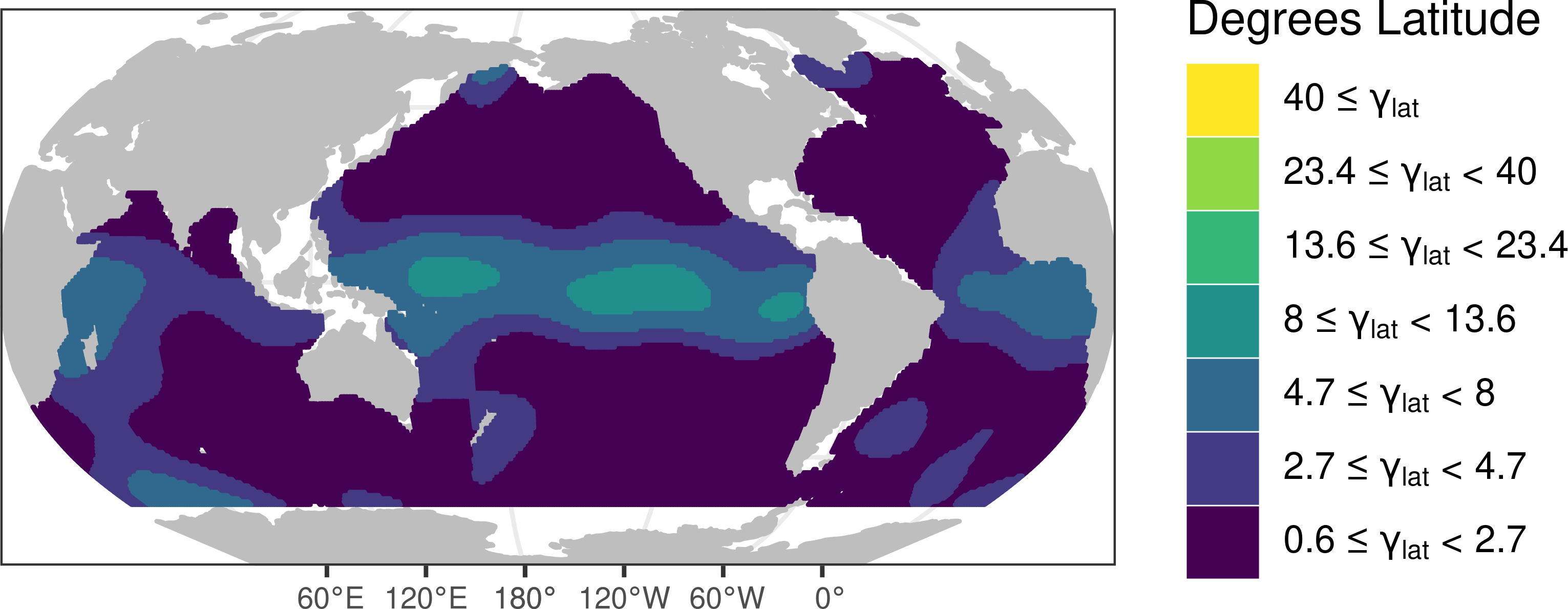
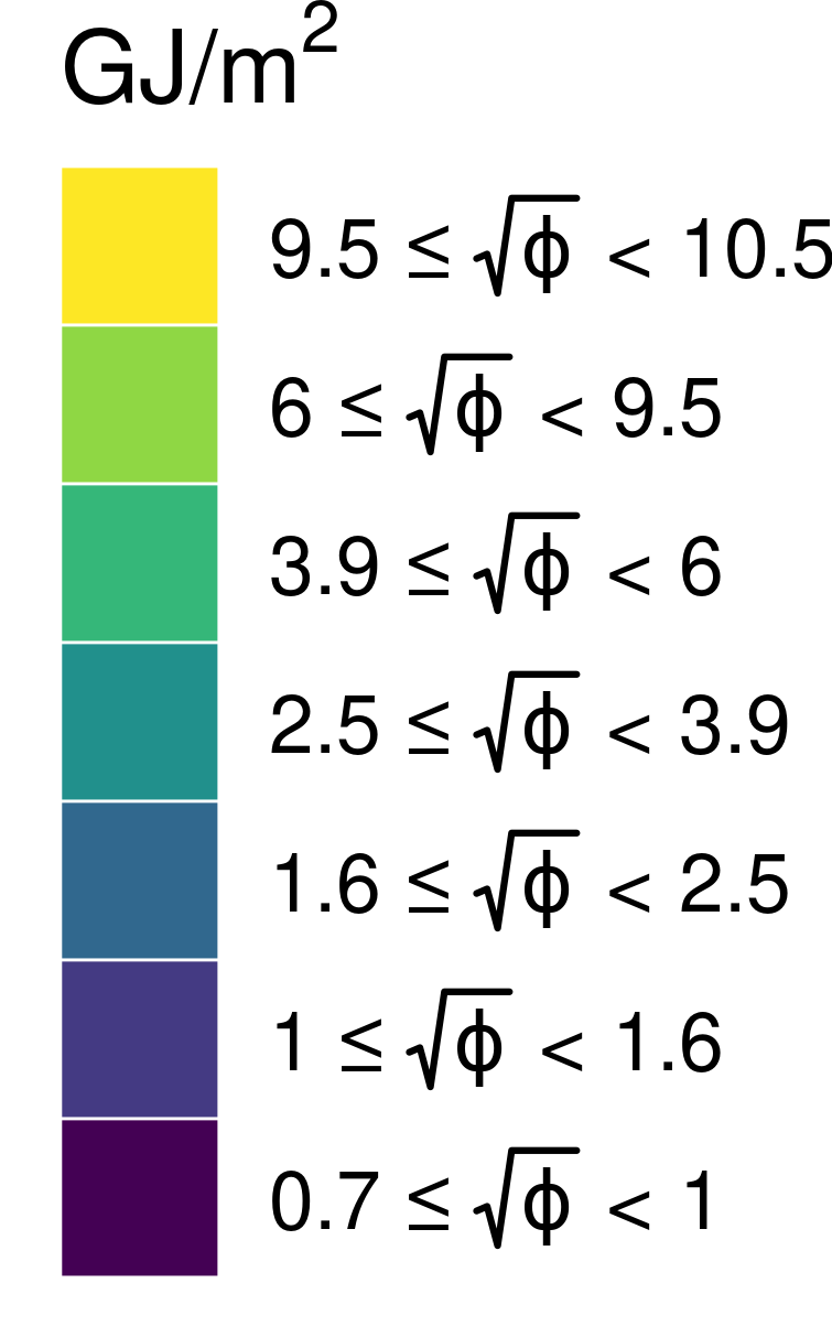
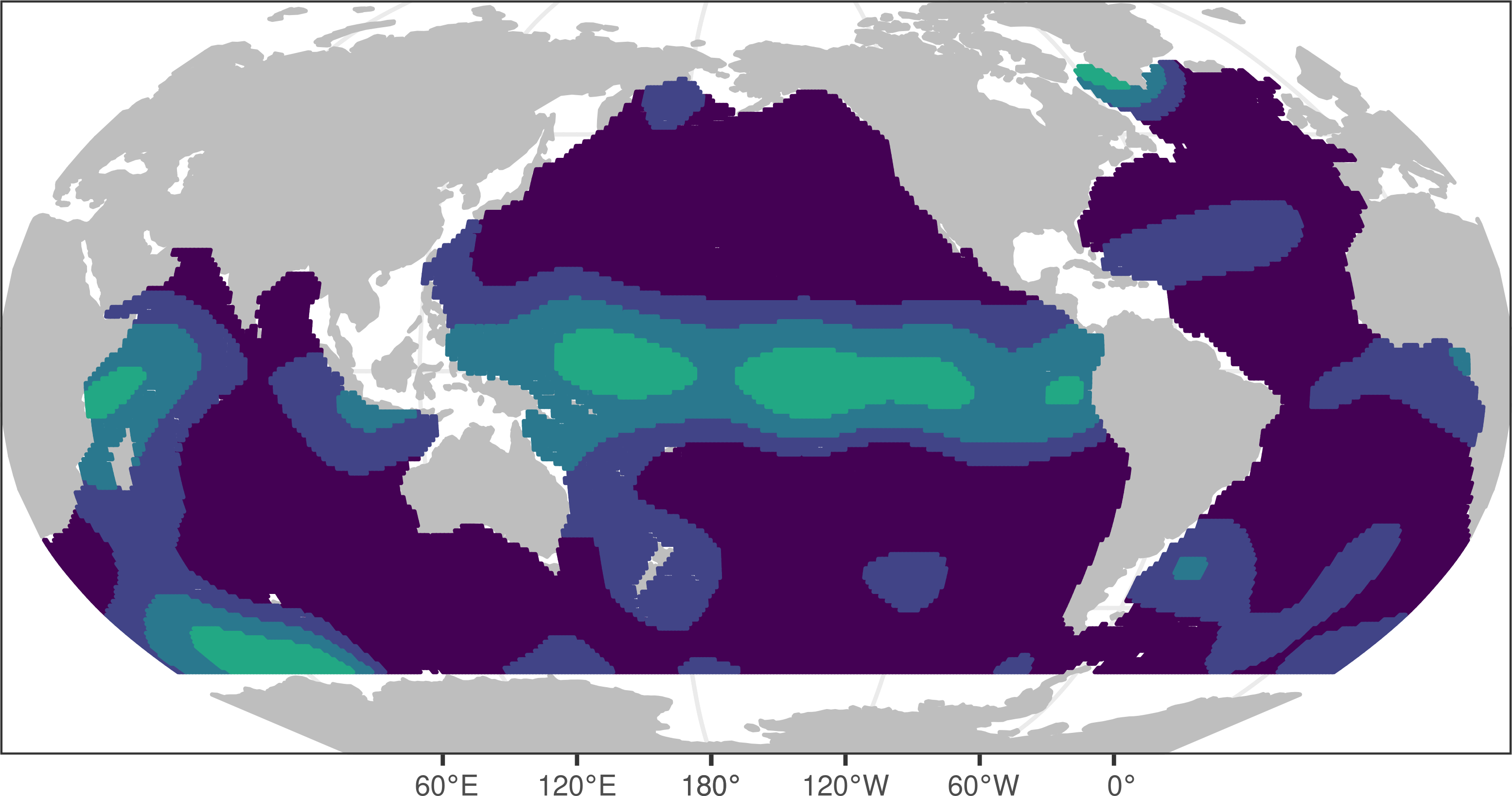
The initial configuration for the MCMC sampler was obtained by kriging the estimated parameters from the moving window approach onto the knot locations using the hyperparameters described in Table 2. Figure 3 displays the initial configuration interpolated over a dense grid for display purposes. Similar to Table 2, standard deviations $\sqrt{\phi}$ and effective ranges $\gamma_{\textnormal{lon}}$ and $\gamma_{\textnormal{lat}}$ are shown rather than the actual parameter fields. While this configuration should not be used to quantify global OHC due to the fact that the estimates were derived assuming local stationarity, comparisons to the 2016 anomaly field displayed in Figure 1(b) yield insights regarding the ocean heat content correlation structure. First of all, we can see from the initial configuration that the correlation length scales around the equatorial regions are much larger than at higher latitudes, and are particularly large in the equatorial Pacific. This phenomenon can be seen in the heat content anomaly field for 2016 through the coherent structures of positive anomalies particularly visible in the eastern equatorial Pacific. These anomalies primarily extend in the longitudinal direction and to a smaller extent in the latitudinal direction. Anisotropy is reflected in the initial configuration, where we can see that the scale of the effective longitudinal correlation lengths is generally much larger than those in the latitudinal plot, a difference that is particularly stark in the equatorial Pacific. The phenomenon of latitudinal correlation lengths being generally smaller than longitudinal correlation lengths makes sense from a physical perspective, as changes in latitude are associated with changes in climate to a much greater degree than changes in longitude.

The areas of the ocean that appear to have particularly high variability in the 2016 anomaly field roughly correspond to the areas of high variance in the initial configuration. Four regions in particular stand out in both of these plots; the North Atlantic east of the United States, the Pacific Ocean east of Japan, the South Atlantic east of Argentina, and a large swath of ocean moving towards the south-east from South Africa to South Australia. We note that most of these regions align with known ocean currents, in particular the Gulf Stream of the North Atlantic, the Kuroshio Current off the coast of Japan, the South Atlantic current off of Argentina, and the Arctic circumpolar current in the Southern Ocean [Colling, 2001]. This is unsurprising, as the currents generate large anomalies of either positive or negative sign depending on the particular position and behavior of the current at a given time.

In theory, the choice of initial configuration will not impact the results of the MCMC sampler if a sufficiently long chain is sampled. However, running the sampler on random initial configurations did not converge after $10{,}000$ iterations. Starting from this initial configuration considerably improves the sampler’s convergence properties as will be discussed in Section 5.2. We have also found that it is particularly challenging to sample the parameter fields and the hyperparameters simultaneously due to the fact that the hyperparameters are not directly informed by the data. To avoid this issue, the hyperparameter values obtained from the moving window approach were treated as fixed and not sampled. This can be interpreted as imposing an informative prior which constrains the variability of the parameter fields to reasonable levels.

Starting from the initial configuration obtained in the previous section, the MCMC sampler was run for $20{,}000$ iterations on a desktop computer with $16GB$ of RAM running Ubuntu 20.04 and using ten cores for the parallel computation of the likelihood evaluations and OHC estimations. The ocean heat content distribution was computed using Equation 9 on a $1^{\circ}\times 1^{\circ}$ grid every ten iterations. To assess convergence, the Heidelberger and Welch test [Heidelberger and Welch, 1981] was run on the sequence of log posterior densities, yielding convergence after a burn-in period of $5{,}401$ iterations. The results that follow are computed on the posterior samples with the burn-in period removed.

To get a sense for the posterior distribution of the parameter fields, for each parameter field we computed the average value across space for each sample and identified fields corresponding to the 5^th and 95^th percentiles of the distribution of mean values. These parameter configurations for the standard deviation $\sqrt{\phi}$, effective latitudinal range $\theta_{\textnormal{lat}}$, and effective longitudinal range $\theta_{\textnormal{lon}}$ are displayed in Figure 4. Note that these are not the point-wise 5th and 95th percentiles of the parameter estimates, which would not retain the spatial structure present in each sample, but rather spatially coherent members of the posterior distribution. The most noticeable difference between these samples and the initial configuration displayed in Figure 3 are the higher longitudinal range parameters in the samples, particularly noticeable in the equatorial West Pacific. This could be due to the fact that the moving-window parameter method may underestimate high values of the range parameter due to the fact that its estimates are based on data from only a $20^{\circ}\times 20^{\circ}$ window. Otherwise, the samples appear to be largely similar to the initial parameter fields, further highlighting the benefit of starting the MCMC sampler at a plausible initial configuration.

While the 5^th and 95^th percentile configurations in Figure 4 are fairly similar to each other for each of the parameter fields, the subtle differences between the percentile maps show that there are regions with higher posterior variability. In the process standard deviation maps in Figure 4(a), differences can be seen in the value and areal extent of the several highly-variable current regions discussed before, indicating some uncertainty in the marginal standard deviation values in these areas. For the longitudinal range maps in Figure 4(b), variability can be seen in the higher-ranged area in the western Pacific, which is the region that changes the most between the initial configuration and the posterior samples. We can also see variability in the distribution of longitudinal ranges in the Southern Ocean, which is likely due to the fact that parameters in this region are more difficult to estimate due to the smaller number of observations near the extent of Antarctic sea ice, as well as the large variability in the data. For the posterior maps for latitudinal range in Figure 4(c), we can see variability in the value and extent of the high-ranged area in the equatorial regions, as well as in smaller areas such as south-east of Argentina and around New Zealand. Overall, however, the variability in the posterior distribution appears to be small for each of the parameter fields, indicating that the uncertainty in the ocean heat content and trend estimations induced by uncertainty in the estimation of the parameters will be relatively low.

The ocean heat content mean and variance were calculated for each year for every ten samples after the burn-in period. For each year, we found the median OHC value over the posterior samples and calculated the 95% confidence interval $\mu_{\textnormal{OHC}_{\textit{yr}}}^{\textnormal{median}}\pm 1.96\sigma_{\textnormal{OHC}_{\textit{yr}}}^{\textnormal{median}}$; these are shown as solid red bars in Figure 5. This represents the uncertainty range induced by the interpolation of the observations to unobserved locations and can be interpreted as a frequentist confidence interval as it does not account for the priors on the parameters. To compute the Bayesian credible interval for each year, for each iteration $t$ of the sampler $100$ heat content values were re-sampled from the marginal OHC distribution $\mathcal{N}(\mu_{\textnormal{OHC}_{\textit{yr}}}^{(t)},\sigma_{\textnormal{OHC}_{\textit{yr}}}^{(t)})$. Then 5^th and 95^th percentiles were computed from the pooled re-resampled OHC values. The re-sampling step ensures that our credible intervals accurately take into account both the interpolation uncertainty from $\sigma_{\textnormal{OHC}_{\textit{yr}}}^{(t)}$ as well as the parameter uncertainty from the variability of $\mu_{\textnormal{OHC}_{\textit{yr}}}^{(t)}$ over the samples. These intervals are displayed as dotted blue bars in Figure 5. We can see that both of the intervals are wider in earlier years, which is to be expected since there are fewer data points in those years. The credible intervals are meaningfully wider than the confidence intervals in earlier years, although the difference becomes small in later years, which is to be expected since the parameter values have a greater effect on the interpolation when there are larger gaps in the data. An analogous procedure was done to obtain uncertainty intervals for the estimated trend; for this parameter, we re-sampled the entire trend field using the posterior covariance matrix conditioned on the other parameters at each iteration. To obtain the 95% credible interval we identified the 2.5% and 97.5% percentiles of the integrated trend values over the re-sampled fields. The 95% confidence interval, computed with the configuration corresponding to the median integrated trend value, is displayed with solid red lines in Figure 5, while the 95% credible interval is displayed as dotted blue lines. The globally integrated trend is positive and highly significant, with a p-value of $.00165$ obtained from the credible interval.

In re-sampling not just the globally integrated trend values but the entire field, we are able to obtain additional information about the spatial variability in the ocean heat content trend. Figure 6 displays samples of the trend fields whose globally integrated values equal the $5$th (panel a) and $95$th (panel b) percentiles of the re-sampled distribution. We can see that variability in the trend field is higher than that in the correlation and variance parameters in Figure 4. Notable features include the cooling trend in the western Pacific and the warming trend in the eastern Pacific, although there appears to be variability in the intensity and areal extent of these trends. There is more confidence in a warming trend in the ocean south-east of Brazil with little apparent variation in the intensity or spatial extent between the two percentile maps. The North Atlantic, on the other hand, displays variable spatial patterns, with the $5$th percentile field showing a negative trend southeast of the United States that is not present in the $95$th percentile map, and while the two percentile fields agree on a cooling trend in the far North Atlantic they differ on its intensity. Other regions where the trend pattern appears largely uncertain are in the Indian Ocean and the Southern Ocean.

These two percentile maps can only give an approximate view of the variability in the trend field, as there is a high-dimensional space of fields whose globally integrated values lie at the $5$th and $95$th percentiles of the posterior distribution. To obtain a better idea of agreement in the posterior we calculated the percentage of the re-sampled trend fields that agree on the sign of the trend for each grid-cell of a $1^{\circ}\times 1^{\circ}$ grid. This is equivalent to the posterior probability of a positive trend value, or $P(\beta(x)>0|\textnormal{observations})$, and the results are displayed in Figure 6(c). We can see that there is agreement on certain spatial features such as the western Pacific cooling trend and the eastern Pacific warming trend. As expected, there is high-level agreement on the warming trend in the ocean south-east of Brazil, and while there is agreement on a positive trend region in the mid-latitude North Atlantic and on the cooling trend in the high-latitude North Atlantic there is no agreement on the trend in the area of the ocean south-east of the United States. There is not any strong agreement on general trends in the Indian and Southern Oceans, however, there are isolated bubbles of confident warming and cooling scattered throughout these regions. We do not expect that these small-scale features would remain significant if more years of observations were used to fit the model, which is reserved for future work.

References

- Trenberth et al. [2014] Kevin E. Trenberth, John T. Fasullo, and Magdalena A. Balmaseda. Earth’s energy imbalance. Journal of Climate, 27(9):3129–3144, 2014.
- Riser et al. [2016] Stephen C. Riser, Howard J. Freeland, Dean Roemmich, Susan Wijffels, Ariel Troisi, Mathieu Belbéoch, Denis Gilbert, Jianping Xu, Sylvie Pouliquen, Ann Thresher, Pierre-Yves Le Traon, Guillaume Maze, Birgit Klein, M. Ravichandran, Fiona Grant, Pierre-Marie Poulain, Toshio Suga, Byunghwan Lim, Andreas Sterl, Philip Sutton, Kjell-Arne Mork, Pedro Joaquín Vélez-Belchí, Isabelle Ansorge, Brian King, Jon Turton, Molly Baringer, and Steven R. Jayne. Fifteen years of ocean observations with the global Argo array. Nature Climate Change, 6:145–153, January 2016. URL https://doi.org/10.1038/nclimate2872.
- Meyssignac et al. [2019] Benoit Meyssignac, Tim Boyer, Zhongxiang Zhao, Maria Z. Hakuba, Felix W. Landerer, Detlef Stammer, Armin Köhl, Seiji Kato, Tristan L’Ecuyer, Michael Ablain, et al. Measuring global ocean heat content to estimate the earth energy imbalance. Frontiers in Marine Science, 6:432, 2019.
- von Schuckmann and Le Traon [2011] Karina von Schuckmann and Pierre-Yves Le Traon. How well can we derive global ocean indicators from Argo data? Ocean Science, 7(6):783–791, 2011.
- Gouretski [2018] Viktor Gouretski. World ocean circulation experiment–Argo global hydrographic climatology. Ocean Science, 14(5):1127–1146, 2018.
- Levitus et al. [2012] Sydney Levitus, John I. Antonov, Tim P. Boyer, Olga K. Baranova, Hernan Eduardo Garcia, Ricardo Alejandro Locarnini, Alexey V. Mishonov, James R. Reagan, Dan Seidov, Evgeney S. Yarosh, and Melissa M. Zweng. World ocean heat content and thermosteric sea level change (0–2000 m), 1955–2010. Geophysical Research Letters, 39(10), 2012.
- Ishii et al. [2017] Masayoshi Ishii, Yoshikazu Fukuda, Shoji Hirahara, Soichiro Yasui, Toru Suzuki, and Kanako Sato. Accuracy of global upper ocean heat content estimation expected from present observational data sets. Sola, 13:163–167, 2017.
- Cheng and Zhu [2016] Lijing Cheng and Jiang Zhu. Benefits of CMIP5 multimodel ensemble in reconstructing historical ocean subsurface temperature variations. Journal of Climate, 29(15):5393–5416, 2016.
- Balmaseda et al. [2013] Magdalena A. Balmaseda, Kevin E Trenberth, and Erland Källén. Distinctive climate signals in reanalysis of global ocean heat content. Geophysical Research Letters, 40(9):1754–1759, 2013.
- Palmer et al. [2017] Matthew D. Palmer, Chris D. Roberts, Magdalena A. Balmaseda, et al. Ocean heat content variability and change in an ensemble of ocean reanalyses. Climate Dynamics, 49(3):909–930, 2017.
- Stein [1999] Michael L. Stein. Interpolation of Spatial Data: Some Theory for Kriging. Springer, New York, 1999.
- Kuusela and Stein [2018] Mikael Kuusela and Michael L. Stein. Locally stationary spatio-temporal interpolation of Argo profiling float data. Proceedings of the Royal Society A: Mathematical, Physical and Engineering Sciences, 474(2220):20180400, 2018. URL https://royalsocietypublishing.org/doi/abs/10.1098/rspa.2018.0400.
- Cheng et al. [2017] Lijing Cheng, Kevin E. Trenberth, John Fasullo, Tim Boyer, John Abraham, and Jiang Zhu. Improved estimates of ocean heat content from 1960 to 2015. Science Advances, 3(3), 2017. URL https://advances.sciencemag.org/content/3/3/e1601545.
- Dijkstra [2008] Henk A. Dijkstra. Dynamical Oceanography. Springer, November 2008. ISBN 3540763759. URL https://www.xarg.org/ref/a/3540763759/.
- Jeong et al. [2017] Jaehong Jeong, Mikyoung Jun, and Marc G. Genton. Spherical process models for global spatial statistics. Statistical science: a review journal of the Institute of Mathematical Statistics, 32(4):501, 2017.
- Higdon [1998] David Higdon. A process-convolution approach to modelling temperatures in the north atlantic ocean. Environmental and Ecological Statistics, 5(2):173–190, 1998.
- Paciorek and Schervish [2006] Christopher J. Paciorek and Mark J. Schervish. Spatial modelling using a new class of nonstationary covariance functions. Environmetrics, 17(5):483–506, 2006. ISSN 1180-4009. URL https://www.ncbi.nlm.nih.gov/pubmed/18163157.
- Risser [2016] Mark D. Risser. Nonstationary spatial modeling, with emphasis on process convolution and covariate-driven approaches. arXiv preprint arXiv:1610.02447, 2016.
- Jeong and Jun [2015] Jaehong Jeong and Mikyoung Jun. A class of matérn-like covariance functions for smooth processes on a sphere. Spatial Statistics, 11:1–18, 2015.
- Li and Zhu [2016] Yang Li and Zhengyuan Zhu. Modeling nonstationary covariance function with convolution on sphere. Computational Statistics and Data Analysis, 104:233–246, 2016. ISSN 0167-9473. URL http://www.sciencedirect.com/science/article/pii/S0167947316301566.
- Sampson and Guttorp [1992] Paul D. Sampson and Peter Guttorp. Nonparametric estimation of nonstationary spatial covariance structure. Journal of the American Statistical Association, 87(417):108–119, 1992.
- Hitczenko and Stein [2012] Marcin Hitczenko and Michael L. Stein. Some theory for anisotropic processes on the sphere. Statistical Methodology, 9:211–227, 03 2012.
- Lindgren et al. [2011] Finn Lindgren, Håvard Rue, and Johan Lindström. An explicit link between gaussian fields and gaussian markov random fields: the stochastic partial differential equation approach. Journal of the Royal Statistical Society: Series B (Statistical Methodology), 73(4):423–498, 2011.
- Turek and Risser [2019] Daniel Turek and Mark D. Risser. BayesNSGP: Bayesian Analysis of Non-Stationary Gaussian Process Models, October 2019. URL https://CRAN.R-project.org/package=BayesNSGP.
- Risser and Turek [2020] Mark D. Risser and Daniel Turek. Bayesian inference for high-dimensional nonstationary Gaussian processes. Journal of Statistical Computation and Simulation, 90(16):2902–2928, November 2020. ISSN 0094-9655.
- Risser [2020] Mark Risser. Nonstationary Bayesian modeling for a large data set of derived surface temperature return values. arXiv:2005.03658 [stat], April 2020. URL http://arxiv.org/abs/2005.03658.
- Katzfuss and Guinness [2021] Matthias Katzfuss and Joseph Guinness. A general framework for Vecchia approximations of Gaussian processes. Statistical Science, 36(1):124–141, 2021.
- Roemmich and Gilson [2009] Dean Roemmich and John Gilson. The 2004–2008 mean and annual cycle of temperature, salinity, and steric height in the global ocean from the Argo program. Progress in Oceanography, 82(2):81 – 100, 2009. ISSN 0079-6611. URL http://www.sciencedirect.com/science/article/pii/S0079661109000160.
- Colling [2001] Angela Colling. Ocean circulation, volume 3. Butterworth-Heinemann, 2001.
- Katzfuss [2013] Matthias Katzfuss. Bayesian nonstationary spatial modeling for very large datasets. Environmetrics, 24(3):189–200, 2013.
- Roberts and Rosenthal [2009] Gareth O. Roberts and Jeffrey S. Rosenthal. Examples of adaptive MCMC. Journal of Computational and Graphical Statistics, 18(2):349–367, 2009.
- Vecchia [1988] Aldo V. Vecchia. Estimation and model identification for continuous spatial processes. Journal of the Royal Statistical Society: Series B (Methodological), 50(2):297–312, 1988.
- Guinness [2018] Joseph Guinness. Permutation and grouping methods for sharpening gaussian process approximations. Technometrics, 60(4):415–429, 2018.
- Datta et al. [2016] Abhirup Datta, Sudipto Banerjee, Andrew O. Finley, and Alan E. Gelfand. Hierarchical nearest-neighbor Gaussian process models for large geostatistical datasets. Journal of the American Statistical Association, 111(514):800–812, 2016.
- Katzfuss et al. [2020a] Matthias Katzfuss, Joseph Guinness, Wenlong Gong, and Daniel Zilber. Vecchia approximations of Gaussian-process predictions. Journal of Agricultural, Biological and Environmental Statistics, 25(3):383–414, 2020a.
- Heidelberger and Welch [1981] Philip Heidelberger and Peter D. Welch. A spectral method for confidence interval generation and run length control in simulations. Communications of the ACM, 24(4):233–245, 1981.
- Gneiting et al. [2005] Tilmann Gneiting, Adrian E. Raftery, Anton H. Westveld III, and Tom Goldman. Calibrated probabilistic forecasting using ensemble model output statistics and minimum CRPS estimation. Monthly Weather Review, 133(5):1098–1118, 2005.
- Guinness and Katzfuss [2018] Jopseh Guinness and Matthias Katzfuss. GpGp: Fast Gaussian process computation using Vecchia’s approximation. R package version 0.1. 0, 2018.
- Katzfuss et al. [2020b] Matthias Katzfuss, Marcin Jurek, Daniel Zilber, Wenlong Gong, Joseph Guinness, Jingjie Zhang, and Florian Schäfer. GPvecchia: Fast Gaussian-process inference using Vecchia approximations. R package version 0.1, 3, 2020b.
- Guinness [2021] Joseph Guinness. Gaussian process learning via Fisher scoring of Vecchia’s approximation. Statistics and Computing, 31(3):1–8, 2021.