Hierarchical-Absolute Reciprocity Calibration for Millimeter-wave Hybrid Beamforming Systems
Abstract
In time-division duplexing (TDD) millimeter-wave (mmWave) massive multiple-input multiple-output (MIMO) systems, the reciprocity mismatch severely degrades the performance of the hybrid beamforming (HBF). In this work, to mitigate the detrimental effect of the reciprocity mismatch, we investigate reciprocity calibration for the mmWave-HBF system with a fully-connected phase shifter network. To reduce the overhead and computational complexity of reciprocity calibration, we first decouple digital radio frequency (RF) chains and analog RF chains with beamforming design. Then, the entire calibration problem of the HBF system is equivalently decomposed into two subproblems corresponding to the digital-chain calibration and analog-chain calibration. To solve the calibration problems efficiently, a closed-form solution to the digital-chain calibration problem is derived, while an iterative-alternating optimization algorithm for the analog-chain calibration problem is proposed. To measure the performance of the proposed algorithm, we derive the Cramér-Rao lower bound on the errors in estimating mismatch coefficients. The results reveal that the estimation errors of mismatch coefficients of digital and analog chains are uncorrelated, and that the mismatch coefficients of receive digital chains can be estimated perfectly. Simulation results are presented to validate the analytical results and to show the performance of the proposed calibration approach.
Index Terms:
Calibration, hybrid beamforming, massive MIMO, millimeter-wave, reciprocity mismatch.Introduction In time-division duplexing (TDD) massive multiple-input multiple-output (MIMO) systems, the base station (BS) estimates the downlink channel state information (CSI) by exploiting the reciprocity of the wireless channel, to relieve the overhead of acquiring CSI[1, 2].
In practice, the estimated CSI is composed of not only the wireless propagation channel response but also the radio frequency (RF) response of RF chains [3]. The transmit and receive RF chains consist of different RF components. The transmit chain is composed of a digital-to-analog converter, a power amplifier, etc., while the receive RF chain consists of an analog-to-digital converter, a low noise amplifier, etc. Due to the different compositions, the RF responses of transmit and receive chains are generally asymmetric, which results in the reciprocity mismatch of the uplink and downlink channels [4].
The study of reciprocity mismatch has attracted extensive attention in the past decade and can be mainly classified into impact analysis and calibration design. To examine the impact of the reciprocity mismatch, some theoretical analyses have been provided for massive MIMO systems with linear precoding techniques, e.g., the zero-forcing (ZF) and matched filter (MF). W. Zhang et al. in [5] studied the performance of the multi-user massive MIMO system with regularized ZF and MF precoding. They found that the reciprocity mismatch hardly caused any performance loss in the low signal-to-noise ratio (SNR) regime but severe performance loss in the high SNR regime. The theoretical results in [6] revealed that the reciprocity mismatch at the BS side was the key contributing factor to the multi-user interference and led to severe system performance degradation for the ZF precoding, while the mismatch at the user equipment (UE) side only led to very slight performance loss. Further, the theoretical comparison of MF and ZF precoding in [7, 8] indicated that the ZF-precoded system was more sensitive to the reciprocity mismatch than the MF-precoded system. The experimental results in [9] verified the theoretical conclusions of the system performance in the presence of the reciprocity mismatch.
Since the reciprocity mismatch causes severe system performance degradation, the reciprocity calibration plays an essential role in the deployment of the massive MIMO system. Unlike the CSI estimation error [10], which changes with each channel realization, the reciprocity mismatch coefficients remain constant over hours or even days, and reciprocity calibration can be performed infrequently, e.g., once an hour. Reciprocity calibration techniques can be mainly classified into two categories, which are hardware-based calibration and over-the-air (OTA) calibration. The hardware-based calibration utilizes the auxiliary circuits and components to connect the transmit RF chains and the receive RF chains. A real-time hardware-based calibration was first proposed in [11] for narrowband conventional MIMO systems, where the transmitted data signals were used to calibrate the antenna array. Then, A. Bourdoux et al. in [12] proposed a calibration approach which calibrated the different subcarriers respectively for wideband systems. To reduce transceiver interconnection effort, a daisy chain interconnection structure of the hardware circuits was proposed in [13], which also reduces the hardware cost of realizing reciprocal calibration to a certain extent. To study the trade-off between the connection structure and performance of the hardware-based calibration, X. Luo et al. in [14] proposed an optimal interconnection by minimizing the Cramér-Rao lower bound (CRLB) of mismatch coefficients, which revealed that the star structure of hardware circuits was optimal. The hardware cost and circuit complexity of these hardware-based calibration methods increase with the number of antennas and may be unaffordable in the massive MIMO systems.
Different from the hardware-based calibration, the OTA calibration is based on the software and protocol design, which only utilizes air-interface signals between uncalibrated antennas to compute the calibration coefficients [15]. OTA calibration approaches can be divided into the full-end OTA calibration which was mainly used for conventional MIMO systems, and the partial-end OTA calibration which was designed for massive MIMO systems. In conventional systems, the OTA calibration requires both the BS and UE to get involved in the operation, and is therefore known as the full-end calibration. The full-end reciprocity calibration was first proposed in [16], and the total least squares (LS) algorithm was applied to solve calibration coefficients. Then, in [17], the full-end calibration was extended to OFDM systems with each subcarrier calibrated independently in the frequency domain. In this case, the overhead and complexity of the reciprocity calibration increased with the number of subcarriers. To reduce the overhead and complexity, B. Kouassi et al. in [18] proposed a time-domain calibration for OFDM systems because the number of coefficients in the time domain was much less than those in the frequency domain. Since the overhead of channel feedback increases with the antenna number, the full-end calibration would produce heavy overhead pressure in massive MIMO systems.
Thanks to the theoretical and experimental results that the reciprocity mismatch at the single-antenna UE only causes minor performance loss, the OTA calibration only needs to be performed at the BS side, which is known as the partial-end calibration or one-side calibration. C. Shepard et al. in [19] proposed a simple one-side calibration for the massive MIMO Argos prototype, which was sensitive to the fading channel and the location of the reference antenna. To avoid the issue of the Argos calibration, a partial-end calibration based on the strong mutual coupling between the adjacent antennas was presented in [20]. By summarizing existing partial-end calibration approaches, X. Jiang et al. proposed an OTA calibration framework in [21]. Compared with co-located system, the calibration in distributed systems needs to gather the CSI from access points (APs). To reduce the overhead of gathering the CSI, R. Roganlin et al. in [22] proposed a hierarchical calibration which consisted of the intra-calibration and inter-calibration of AP. In [23], an OTA calibration with supporters was proposed for coordinated multi-point transmission systems to improve the SNR of calibration signals. To combat the path loss between the APs, our work in [24] proposed a beamforming-based OTA calibration for distribution MIMO relaying systems.
Although the reciprocity calibration designs for full-digital beamforming (DBF) MIMO systems have been extensively investigated in recently, they can not be applied to the hybrid analog-digital beamforming (HBF) systems. Due to the more complex structure than DBF systems, the reciprocity calibration in HBF systems is more challenging. On one hand, a typical HBF transceiver possesses a hierarchical structure consisting of the digital precoder, digital RF chains, the analog precoder, and analog RF chains[25], which results in more complex modeling of the uplink-downlink channel reciprocity mismatch. On the other hand, the digital RF chains and the analog RF chains are coupled with the analog precoder, e.g., a phase-shifter network[26], so that the digital chains and analog chains can not transmit signals independently. A reciprocity calibration for the sub-connected phase-shifter network HBF system was proposed in [27], which transformed the sub-connected HBF transceiver to a DBF transceiver by virtually changing the position of the RF components to the front end near the antennas. When it is applied to the fully-connected HBF system, the dimension of the equivalent channel matrix after the transformation becomes much larger than the realistic channel, which results in a large overhead of the calibration. Additionally, since this reciprocity calibration can only acquire the ratio of coefficients of transmit and receive RF chains, mmWave channel estimation approaches, e.g., the approaches in [28, 29, 30] which requires mismatch coefficients rather their ratios, remain unusable. To reduce the overhead and recover the mmWave channel estimation, a relative reciprocity calibration approach was proposed for fully-connected mmWave HBF system in [31]. Although this approach can reduce the calibration overhead to a certain extent, it requires UE to feed back received downlink calibration signals to BS, which can still causes large overhead. Further, since the relative calibration can not construct the equivalent channel, some existing hybrid beamforming designs, e.g. the designs proposed in [32, 33, 34], cannot be applied in the calibrated systems.
Motivated by the above observations, we investigate the reciprocity calibration for TDD mmWave-HBF systems with the fully-connected phase shifter network. To reduce the overhead and complexity of the reciprocity mismatch in the fully-connected HBF system, hierarchical ideology is employed to calibrate digital and analog RF chains. Since digital and analog RF chains are physically coupled via a phase shifter network, we propose a beamforming design to virtually decouple the reciprocity calibration of digital and analog RF chains. Based on the decoupling operation, the entire reciprocity calibration problem is decoupled into two subproblems corresponding to the calibrations of digital RF chains and analog RF chains. To guarantee the application of mmWave channel estimation approaches, we propose an absolute reciprocity calibration approach to estimate the mismatch coefficients of transmit and receive RF chains. The mismatch coefficients of digital RF chains are solved from the closed-form expression of the solution to the digital-chain problem, while the mismatch coefficients of analog chains are jointly estimated with mmWave channel coefficients. Finally, the CRLB of the mismatch coefficients is derived to measure the performance of the proposed calibration. The main contributions of this work can be summarized as follows.
-
•
Reciprocity mismatch decoupling. Since digital and analog RF chains are physically coupled via a phase shifter network, we propose a beamforming design to virtually decouple the digital and analog RF chains. Then, the entire reciprocity mismatch calibration problem of the HBF system is decomposed into two separate problems of digital-chain calibration and analog-chain calibration.
-
•
Absolute reciprocity calibration. To guarantee the efficacy of mmWave-channel estimation approaches, we propose novel estimating methods to acquire the mismatch coefficients of RF chains. Specifically, the closed-form expression of digital-chain mismatch coefficients is derived, and an iterative-alternating estimation algorithm is proposed for analog-chain mismatch coefficients.
-
•
CRLB for estimating mismatch coefficients. To measure the performance of the proposed algorithms, we derive the CRLB for the mismatch coefficient estimation. The CRLB reveals that the errors in estimating mismatch coefficients of digital chains and analog chains are independent of each other, and the mismatch coefficients of receive digital chains can be estimated perfectly.
The rest of the paper is organized as follows. Section II describes the system model. The hierarchical-absolute reciprocity calibration for the mmWave-HBF system is proposed in Section III. In Section IV, the performance including the overhead, computational complexity, and CRLB of the proposed calibration is derived. Simulation results are given in Section V, and the conclusion is given in Section VI. For readability, some proofs are deferred to the supplementary material.
Throughout the paper, vectors and matrices are denoted in bold lowercase and uppercase respectively, e.g., and . Let , , and denote the transpose, conjugate transpose, and inverse of a matrix respectively. , , and stand for the trace operator, the expectation operation, and column vectorization. Let and denote the amplitude and phase of the complex number , and denotes the Frobenius norm. denotes an by diagonal matrix with diagonal entries given by , and represents a block diagonal matrix. , , and represent the Kronecker product, Khatri–Rao product, and Hadamard product, respectively. and stand for the complex numbers and real numbers, respectively. Let denote the set , and denote the remainder of divided by .
I System Model
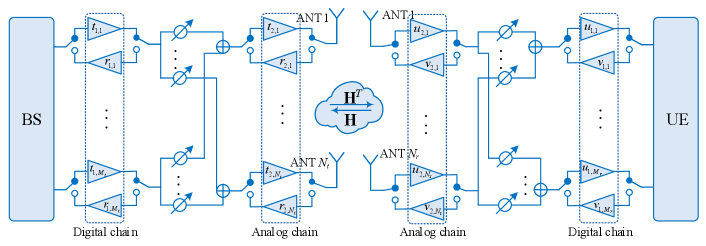
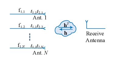
We consider an mmWave massive MIMO system as illustrated in Fig. 1, where the BS is assumed to communicate with a single UE. The BS is quipped with digital RF chains and analog RF chains, and the UE is equipped with digital RF chains and analog RF chains. In both BS and UE, each analog chain is connected to an antenna in the uniform linear array (ULA), and the digital chains are connected to the analog chains via a fully-connected phase shift network.
In mmWave systems, the wireless channel is generally considered to possess limited scattering. Thus, we adopt a geometric channel model with scatters, and each scatter contributes to a single propagation path between the BS and UE. Based on these assumptions, the wireless channel between the BS and the UE can be modeled as
| (1) |
where is the complex gain of the -th path, and denote the array steering vectors of the BS and UE which are given by
| (2) |
is the wavelength of the carrier, and is the distance of the adjacent antenna set to , and are the azimuth angles of arrival or departure (AoAs/AoDs) of the BS and MS.
In a practical system, the receive and transmit RF chains are generally asymmetric. Let and represent the mismatch matrices of the transmit/receive digital and analog RF chains of the BS, and denote and as the mismatch matrices of the transmit/receive digital and analog RF chains of the UE. All of these matrices are diagonal and defined as
| (3) |
where denotes the mismatch coefficient of the -th () transmit/receive digital RF chain of the BS, and denotes the mismatch coefficient of the -th () transmit/receive analog RF chain of the BS. At the UE side, denotes the mismatch coefficient of the -th () transmit/receive digital RF chain, and denotes the mismatch coefficient of the -th () transmit/receive analog RF chain.
As depicted in Fig. 1, the overall channel observed by the baseband processor is the combination of the wireless channel, the digital RF chain, the phase shifter network, and the analog RF chain, which can be expressed by
| (4) |
where , , and are the analog receive and transmit beamforming matrices of the BS, , , and are the analog beamforming matrices of the UE.
Based on the channel modeling and system setting, the downlink transmission signal received by the UE can be denoted as
| (5) |
where is the digital combining matrix of the UE, denotes the digital precoding matrix of the BS, denotes the data vector satisfying , denotes the average transmit power, is the number of data streams, and represents the additive white Gaussian noise (AWGN) vector with distribution .
In TDD mode, the digital and analog beamforming matrices are computed by the BS based on the knowledge of uplink CSI. According to (4), the estimated uplink CSI is unequal to the downlink channel response at all, which is known as the reciprocity mismatch of the uplink and downlink channel. With the reciprocity mismatch, the existing beamforming approaches for HBF systems, e.g., [35], fail to achieve satisfactory performance. Further, due to the uncertainty of the reciprocity mismatch coefficients, mmWave channel estimation approaches like [28] are invalid. Accordingly, the reciprocity calibration is essential for mmWave-HBF systems.
II Reciprocity Calibration for mmWave-HBF System
In this section, the reciprocity calibration approach is proposed. We first introduce an existing reciprocity calibration approach for HBF systems and discuss its limitation in applying to the fully-connected structure. Then, an absolute reciprocity calibration for the mmWave-HBF system is proposed, which takes advantage of the particularity of the fully-connected structure to decouple the calibrations of digital RF chains and analog RF chains.
II-A Conventional Reciprocity Calibration Approach of HBF System
The conventional reciprocity calibration (CRC) of HBF was proposed in [27], which is an extension of the relative calibration of the full-digital MIMO system. The CRC treats the HBF system as a virtual full-digital MIMO with virtual antennas and applies OTA signals to estimate the ratio of the transmit and receive mismatch coefficients, which are also called relative calibration coefficients.
In the CRC, the equivalent transmit and receive mismatch coefficients of the BS are defined as and , and the equivalent mismatch coefficients of the UE are defined as and . The equivalent uplink and downlink channels are defined as and , where , , , and consist of the diagonal entries of , , , and , respectively. Based on these definitions, the equation of CRC can be denoted as
| (6) |
where and represent the relative calibration matrices of the BS and UE.
To obtain the relative calibration coefficients, it is necessary to acquire the equivalent uplink and downlink CSI. To estimate the equivalent downlink CSI, the BS transmits -length pilots by using transmit beamforming matrices, and the UE receives the pilots with receive beamforming matrices, where . Assume that a -length pilot sequence is denoted as , where denotes the pilot during the -th transmission satisfying . During the training, the digital precoding and combining matrices are set as identity matrices, i.e., and , and the signal received by the UE can be denoted as
| (7) |
where , denotes the analog beamforming matrix at the BS, is the analog combining matrix at the UE, , denotes the -th column of , , and is the -th row of .
By stacking all -length signals in matrix form denoted as and , the received signal model can be given by
| (8) |
where , , , and . By vectoring the matrix , the received signal can be further denoted as
| (9) |
where . Using the LS approach[36], the equivalent downlink channel is estimated as
| (10) |
Similarly, to estimate the equivalent uplink channel, the UE transmit the uplink training pilots to the BS. Further, to estimate the calibration coefficients, the UE feeds back the estimated downlink channel to the BS.
After the BS estimates the uplink channel and receives the downlink channel fed back from the UE, the calibration coefficients can be computed by the following proposition.
Proposition 1 (CRC coefficients).
With the knowledge of the equivalent uplink and downlink channels, the CRC coefficients can be computed by
| (11) |
where is the first column of matrix , consists of the second to last columns of matrix , is an -order square matrix defined as .
Proof:
The results can be derived based on [27] by assuming that the antennas of the BS are divided into the group and the antennas of the UE are divided into the group . ∎
To measure the complexity of the CRC, we further derive the overhead and computational complexity. The overhead of reciprocity calibration can be expressed by the count of channel use for transmitting calibration signals and feeding back the estimated CSI. The computational complexity can be measured by the times of multiplication for estimating the channel state information and computing the mismatch coefficients.
Remark 1 (Overhead and complexity of CRC).
According to (10), must be a full column rank matrix to estimate the downlink channel. Based on the property of the Kronecker product, the pilots must satisfy the condition that and , and . This result means that the least overhead of downlink channel estimation is . Since the uplink channel estimation is similar to the downlink channel estimation, the entire overhead of the CRC can be denoted as . Further, since the computation complexity is mainly determined by computing the inverse matrices of and , the computation complexity of the CRC is .
In the CRC, the dimensions of the equivalent channels and (see (6)) are much larger than that of the actual wireless channel matrix (see (1)), which generates the heavy overhead of the channel estimation and high computational complexity. Further, since the CRC only estimates the ratio of the mismatch coefficients of transmit chains and receive chains, mmWave channel estimation of mmWave systems, which requires the knowledge of the individual mismatch coefficients, becomes invalid. Thus, due to limitations of the CRC in fully connected mmWave-HBF systems, we propose a hierarchical-absolute calibration (HAC) approach, which decouples the reciprocity calibration of digital RF chains and analog RF chains and estimates the individual mismatch coefficients of transmit chains and receive chains, respectively.
II-B Decouple Principle of HAC
To reduce the overhead and complexity of the reciprocity calibration of fully connected HBF systems, digital RF chains and analog RF chains must be calibrated individually, which means hierarchical calibration. To adopt the mmWave channel estimation approaches of mmWave systems, the individual mismatch coefficients are required rather than the ratio of the mismatch coefficients, which can be addressed by applying the absolute reciprocity calibration.
However, due to the fully-connected structure of the HBF system, HAC encounters two challenges. On the one hand, the digital RF chains and analog RF chains are physically coupled via the fully-connected phase shift network, which results in the decoupling challenge. On the other hand, the fully-connected phase shift network causes that the RF chains can not transmit and receive signals independently, which results in the calibration challenge. To a certain degree, these problems can be addressed by using extra auxiliary circuits to assistant the reciprocity calibration, e.g. the calibration approaches presented in [37, 38]. But the auxiliary circuits may bring extra non-reciprocity, and the calibration accuracy of hardware-circuit calibration highly depends on the auxiliary circuits [20]. Thus, we propose an OTA-based HAC for mmWave-HBF systems. Specifically, the calibrations of digital and analog RF chains are decoupled by a targeted beamforming scheme, and the mismatch coefficients are estimated by the OTA training signals between the BS and UE.
In the rest of this section, we will introduce the decoupling principle of the proposed HAC. Since the transmitter and receiver employ similar HBF structures, the decouple operation is first explained in the multi-input single-output (MISO) system for clarity, and then we will propose the concrete design for the general HBF-MIMO system.
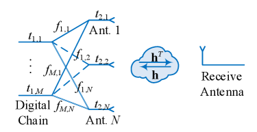
MISO system for decoupling digital chains from the analog chains: We consider a MISO system where the transmitter is equipped with the fully-connected HBF structure and the receiver is equipped with a single antenna as illustrated in Fig. 2a. Thanks to the fully-connected structure, the signal transmitted from each digital RF chain passes through all antennas in the transmitter and all wireless channels. For example, if the -th transmit digital chain transmit a signal to the receiver, the received signal can be denoted as
| (12) |
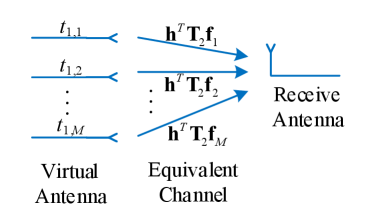
where denotes the virtual equivalent channel between the -th transmit digital chain and the receive antenna. Based on this, the HBF MISO system can be virtually constructed as a DBF MISO system as illustrated in Fig. 2b, where the virtual antennas are the transmit digital chains, and the virtual-equivalent channels consist of the phase shift network, the analog RF chains, and the wireless channel. Further, it can be found that the virtual-equivalent channels equal to each other when the beamforming vectors are identical, i.e., . Thus, by applying this analog beamforming design, the digital chains can be decoupled from the analog chains, and the absolute reciprocity calibration can be considered as the calibration with known channel gains.
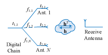
MISO system for decoupling the analog chains from the digital chains: Since each digital RF chain is connected to all analog RF chains via the fully-connected phase shifter network, the antenna array can be considered as an ABF system as shown in Fig. 3a. By using only one digital RF chain to transmit and receive calibration signals, the analog RF chains can be decoupled from the digital RF chains as illustrated in Fig. 3b. Based on this design, the analog RF chains can be calibrated with signal processing approaches.
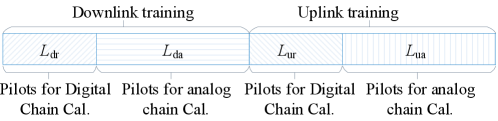
Concrete design: Based on the above MISO systems, the decoupling principle can be extended to a general case where both the BS and UE are equipped with multiple antennas and HBF structures as illustrated in Fig. 1. For general point-to-point HBF MIMO systems, the overall HAC training phases can be divided into two phases, which are downlink training and uplink training as illustrated in Fig. 4. During the training processes, the calibration training signals and beamforming matrices of the BS and UE should be designed to decouple digital and analog RF chains. By taking the downlink training phase as an example, the concrete designs are given as follows.
-
•
Downlink training pilots: The entire -length downlink training pilots consist of -length pilots for calibrating digital RF chains and -length pilots for calibrating the analog RF chains, where . To increase the degree of freedom of received signals, the -length pilots are transmitted by using transmit beamforming matrices and received by using receive beamforming matrices, where . The -length pilots possess the homologous structure, i.e., . By using to represent the pilots set, the transmitted pilot during the -th transmission can be denoted as , where , when , and when , .
-
•
Beamforming design for calibrating digital chains: Let denote the analog transmit beamforming matrix and represent the receive beamforming matrix during the -th transmission, where , , and . To decouple the mismatch of the digital chains from the analog chains, analog beamforming matrices are designed as and , where each element of and possesses random phase. Further, the digital precoding matrix can be designed as and the digital receive combining matrix is given by during the downlink training phase.
-
•
Beamforming design for calibrating analog chains: During the -th transmission (), the analog transmit beamforming matrix and receive beamforming matrix can be designed as random phase matrices, i.e., the elements of and possess random phases. Let denote the digital precoding matrix and denote the digital receive combining matrix, where , and . To decouple the mismatch of analog RF chains from the mismatch of digital RF chains, the digital precoding matrix can be designed as , and the digital receive combining matrix can be given by .
II-C Problem Formulation and Decomposition of HAC
Since the mismatch coefficients of transmit chains have nothing to do with that of receive chains, HAC can be divided into downlink HAC and uplink HAC. The downlink HAC is applied to calibrate the transmit chains of the BS and the receive chains of the UE, while the uplink HAC can calibrate the receive chains of the BS as well as the transmit chains of the UE. The uplink HAC is similar to the downlink HAC. Thus, we introduce the signal modeling, the problem formulation, and the problem decoupling by taking the downlink HAC as an example.
By considering the BS transmits -th pilot to the UE, the signal received by the UE can be modeled as
| (13) |
where . When , , , , and , where , and . When , , , , and , where , and .
After the BS transmits -length pilots to the UE, the optimization problem for jointly estimating , and can be formulated as
| (14) |
where , . Thanks to the proposed pilots and training scheme design, the above joint optimization problem can be equivalently decoupled into two subproblems demonstrated in the following proposition.
Proposition 2 (HAC problem decoupling).
Based on the specific pilots and training scheme design in Section II-B, the problem of HAC in (14) can be equivalently decoupled into two independent problems as
| (15) | |||
| (16) |
where , , consists of the diagonal entries of , is composed of the diagonal entries of , , , , , , , is the first column of , denotes the first column of , and represents the first entry of .
Proof:
See Appendix A. ∎
Remark 2 (HAC decoupling).
Since the problem can solve the mismatch coefficients of the transmit digital RF chains of the BS and those of the receive digital RF chains of the UE, it is known as the downlink calibration problem of digital RF chains. Similarly, the problem is the downlink calibration problem of analog RF chains. Thus, Proposition 2 indicates that HAC can be decoupled into the calibration of digital RF chains and the calibration of the analog RF chains, which is the purpose of the hierarchical calibration.
II-D Solution to Calibration Problem of HAC
As and are independent of each other, we first find the solution to , then solve . As the objective of is bilinear, it can be solved by iterative approaches but this is inefficient. To solve efficiently, we propose a closed-form solution by regarding the first receive digital chain of the UE as the calibration reference.
By using the auxiliary variables and , the problem can be further formulated by
| (17) |
By taking the derivative of the objective function of , the solution can be given by[36]
| (18) |
Since the first receive digital RF chain of the UE is the reference, its mismatch coefficient can be treated as a known constant, e.g., . Based on this assumption and (18), equals to the first column of , i.e.,
| (19) |
where is the -th row of .
By substituting (19) into (15), the solution to the problem can be given in the following proposition.
Proposition 3 (Solutions to the problem ).
By assuming that the first receive digital RF chain is set as the reference, i.e., , the solutions to and can be given by
| (20) | |||
| (21) |
where , consists of the second to the last row of , , and .
Proof:
See Appendix B. ∎
Remark 3 (The special solution to ).
Equations (20) and (21) give the general solutions to and are dependent on the value of . In practice, it is difficult to determine the value of . To avoid this issue, the mismatch coefficient of the reference can be set to , i.e., . In this case, equations (20) and (21) degenerate to a special solution to . Since the vectors parallel to and can be applied to the calibration, the special solution to still works for the reciprocity calibration.
Then, the mismatch coefficients of analog RF chains can be estimated by solving . By exploiting the geometry channel model of mmWave, the calibration problem of analog chains can be further written as
| (22) |
where , , , and . As the variables are correlated with each other, this problem is nonconvex and there is no tractable solution to the problem. To solve efficiently, inspired by [39], we propose an alternating optimization algorithm to solve a locally optimal solution.
During the -th iteration, we apply the least square algorithm to estimate the diagonal matrices , , , then, propose an algorithm to estimate the AoA and AoD matrices , .
Lemma 1 (Solution to the diagonal matrices).
During the -th iteration, when , , and are known, the diagonal elements of can be estimated by
| (23) |
where . When , and , are known, the diagonal elements of can be estimated by
| (24) |
where . Similarly, by giving , , and , the diagonal entries of can be given by
| (25) |
where .
Proof:
The complete proof is presented in Appendix C of Supplementary Material. ∎
Finally, we propose a AoAs and AoDs updating algorithm111The update method of AoA/AoD is not restricted to the algorithm proposed in this paper. Some existing methods, such as those presented in [30], can be employed. when , , , , and are given. Since the AoAs and AoDs can be estimated using the same approaches, we introduce the updating algorithm by taking updating the AoDs as an example. Since the problem for estimating AoDs is nonlinear, it is difficult to solve the AoDs directly. To address this issue, as presented in [40], the nonlinear problem is transformed into a series of linear problems by using the first-order Taylor expansion to approximate the array steering vector. Let denotes the differences between the estimated AoDs and the real AoDs . By assuming that the differences are small, the array steering vector can be approximated by the first-order Taylor expansion denoted as , where . Then, the problem can be further formulated as
| (26) |
where , , , and . The solution can be given by
| (27) |
. Since is assumed to be small, the updating requires several iterations, and the iterative updating algorithm is summarized as Algorithm 1.
It is worth noting that the initial values of AoAs and AoDs can be roughly calculated by direction finding methods, e.g., the modified MUSIC algorithm in [41].
Finally, based on Lemma 1 and Algorithm 1, the problem can be solved by an alternating optimization algorithm, which is summarized as Algorithm 2.
Remark 4 (Convergence analysis).
Similarly, the mismatch coefficients of the receive RF chains of the BS and the transmit RF chains of the UE can be estimated by the uplink calibration. During the uplink calibration, the UE transmits pilots to the BS, and the BS estimates the mismatch coefficients by Proposition 3 and Algorithm 2. With estimated mismatch coefficients, the reciprocity mismatch can be compensated in the digital domain. Thus, the overall procedure of HAC can be summarized as follows.
-
Step 1
(Downlink calibration) The BS sends downlink pilots to the UE. After receiving the downlink pilots, the UE jointly estimates the mismatch coefficients of the transmit RF chains of BS and the receive RF chains of UE by Algorithm 2;
-
Step 2
(Uplink calibration) The UE transmits uplink pilots to the BS. Based on the received uplink pilots, the BS calculates the mismatch coefficients of the receive RF chains of BS and the transmit RF chains of UE with Algorithm 2;
-
Step 3
(Mismatch coefficients feedback) The UE feeds back the estimated mismatch coefficients to the BS, and the BS sends the mismatch coefficients to the UE;
-
Step 4
(Reciprocity mismatch compensation) During data transmission phases, CSI can be estimated by utilizing the knowledge of mismatch coefficients and some existing approaches , e.g., the methods presented in [28, 29, 30]. Then, the equivalent downlink CSI can be formulated as , and the precoding/combining and beamforming matrices can be designed by some existing approaches, e.g. the methods proposed in [32, 33, 34]. Finally, the mismatch of digital RF chains can be compensated by multiplying the inverse of mismatch coefficients matrices of digital chains on the precoding/combining matrices.
II-E Extend HAC to the multi-user scenario
Although the HAC is introduced in a point-to-point HBF system, it can be also applied in multi-user HBF systems, where a single BS serves UEs simultaneously. Each UE is equipped with an HBF transceiver. Same as the single-UE case, the HAC consists of the downlink calibration and the uplink calibration. For both downlink and uplink calibrations, the pilots and beamforming designs remain consistent to the single-UE case.
Downlink calibration: The BS sends training pilots to the UEs, and the -th UE received signal can be denoted as
| (30) |
where denotes the wireless channel between the -th UE and the BS, and are the mismatch coefficient matrices of the receive digital and analog chains of the -th UE. Since (30) of each UE is same as (13), it can be solved by the same approach, i.e., Proposition 2, Proposition 3, and Algorithm 2.
Uplink calibration: The UEs sends training pilots to the BS, and the received signal can be given by
| (31) |
where , , , , , and represent the mismatch matrices of the transmit digital and analog chains of the -th UE. The uplink calibration problem can be formulated as
| (32) |
which can be decomposed into the calibration problem of digital chains and analog chains by Proposition 2. The uplink calibration problem of digital chains can be solved by Proposition 3, whereas the problem of analog chains can not solved by Algorithm 2 due to the different structure of . Fortunately, if UEs feed back AoAs and AoDs estimated in the downlink calibration to the BS, the BS only estimates the mismatch coefficients and which can be solved by alternating optimization approach similar to Algorithm 2.
III Performance Analysis of Reciprocity Calibration
In this section, we will analyze the performance of the proposed HAC. The minimum length of the calibration pilots will be first derived, followed by the overhead and computational complexity analysis. To measure the performance of the proposed calibration approach, the Cramér-Rao lower bound will be derived as the benchmark of the calibration performance.
III-A Overhead and Complexity of HAC
Based on the calibration signal design and estimation approaches, we can derive the requirements of the length of calibration pilots.
Proposition 4 (Length of downlink pilots).
The proposed downlink training and estimation approaches require that the length of pilots meets the following conditions
| (33) |
Proof:
The complete proof is presented in Appendix D of Supplementary Material. ∎
Based on the above pilot requirements and the proposed calibration algorithms, the overhead and computational complexity of HAC can be given in the following lemma.
Remark 5 (Overhead and complexity of the proposed HAC).
By considering the length of pilots exactly meets the requirements denoted as (33), the overhead of downlink training is proportional to . In each iteration , the computational complexity is mainly caused by computing the inverse of matrices. Let denote the total iteration number of updating AoA/AoD and represent the iteration number of Algorithm 2. The complexity of solve problem can be given by . The comparisons between the overhead and complexity of HAC and CRC are shown in Table I, which indicates that the proposed HAC requires requires less overhead. According to experiments, both Algorithm 1 and Algorithm 2 converge after several iterations, and the complexity of the HAC is also lower than the CRC.
| Overhead | Complexity | |
|---|---|---|
| CRC | ||
| HAC |
III-B CRLB of Calibration Coefficients
To verify the performance of proposed joint estimation approaches, we derive the CRLB of , , , and to be the performance benchmark, where . We first define the variable vectors as
| (34) |
| (35) |
and the transformation function vector as
| (36) |
Based on this definition, the CRLB of the equivalent mismatch coefficients can be defined as follows.
Definition 1 (CRLB of ).
According to the transformation relation in [44], the CRLB of can be given by
| (37) |
where denotes the Fisher information matrix of , and is the -th entry of .
Lemma 2 (Transformation of the Fisher information matrix).
By dividing the variables into two parts and defining the vectors and , the Fisher information matrix can be further denoted as
| (38) |
where denotes the Fisher information matrix of , .
Proof:
The complete proof is presented in Appendix E of Supplementary Material. ∎
Thus, to derive the closed-form expressions of the CRLB of , we first derive the closed-form expression of denoted as follows.
Lemma 3 (Closed-form expression of ).
The closed-form expression can be given by
| (39) |
where , , , and .
Proof:
The complete proof is presented in Appendix F of Supplementary Material. ∎
Similarly, for deriving the closed-form expressions of , we derive denoted in the following lemma.
Lemma 4 (Closed-form expression of ).
The closed-form expression of can be given by
| (40) |
where , , , and are defined in Lemma 1, , , and , is the -the column of , , and .
Proof:
The complete proof is presented in Appendix G of Supplementary Material. ∎
Proposition 5 (CRLB of ).
Proof:
The complete proof is presented in Appendix H of Supplementary Material. ∎
Remark 6 (CRLB analysis).
From (41), the CRLB of is equal to zeros. This result is because is estimated from the deterministic signals. The CRLB of can be given by , which indicates that increasing the pilots can improve the accuracy of .
IV Simulation Results and Discussions
In this section, we will provide simulation results to evaluate the performance of the proposed reciprocity calibration approach for the mmWave-HBF system.
The system parameters are set as follows. Analog RF chains of the BS and UE, and the number of data streams are different in each simulation, while the number of digital RF chains equals to a quarter of the number of analog RF chains, i.e., and . The path number of the mmWave channel is set to . The variance of the channel gain is set to , and the AoAs and DoAs obey the uniform distribution, i.e., . Then, the amplitudes of reciprocity mismatch coefficients obey the log-normal distribution, i.e., , and the phases of reciprocity mismatch coefficients follow the uniform distribution, i.e., . Further, the length of pilots is set to , , and . Finally, the variance of the AWGN is , and denotes the average SNR of received calibration signals during the simulation.
IV-A NMSE of Estimated Mismatch Parameters
To illustrate the performance of the proposed HAC calibration approach, we compare the normalized mean square error (NMSE) of the mismatch coefficients with the CRLB. The NMSE of the mismatch coefficients is defined as . It is worth noting that the Oracle HAC represents the reciprocity calibration with the knowledge of AoAs and AODs, which is a performance benchmark of the proposed HAC.
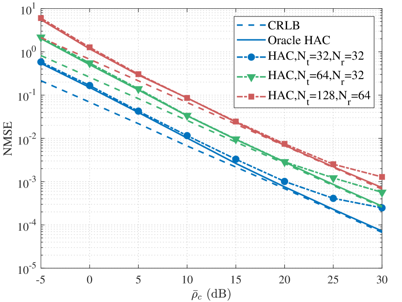
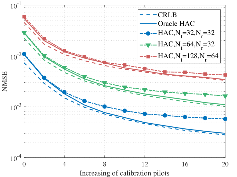
Fig. 6 demonstrates the NMSE of the mismatch coefficients versus the SNR of the calibration signals, where the antenna numbers of the BS and the UE are set to three different sets of parameters given by . It can be seen that the NMSE of the proposed HAC gradually achieves a floor with the increase of calibration SNR. This is because the solution to the nonconvex problem gets stuck in local optima. Further, the figure also shows that the floor effect can be alleviated when the antenna number increases, which is because the independence between array steering vectors increases with the increase of antenna number. Besides, we find that the NMSE increases with the antenna number. This result indicates that the system with more antennas requires higher calibration SNR to guarantee the same calibration performance as the system possessing fewer antennas.
Then, the NMSE of the mismatch coefficients versus the length of calibration pilots is illustrated in Fig. 6 with the SNR of calibration signals set to dB. From the figure, it can be found that the NMSE and CRLB decrease with the increase of calibration pilots, which is consistent with the theoretical results shown in Proposition 5. This result indicates that better performance of the proposed HAC can be achieved at the cost of overhead or power. Also, the curves of the proposed HAC gradually approach floors when the length of pilots increases, while the curves of the Oracle HAC gradually converge to the CRLB. Increasing the antenna number can reduce the floor effect.
IV-B NMSE of Channel Estimation
To examine the efficacy of the reciprocity calibration in mmWave-HBF systems, we study the NMSE of the uplink channel estimation by using the two-dimension MUSIC algorithm proposed in [28], and the pilot block is set to .The NSME of the estimated channel is defined as
| (43) |
where denotes the estimated channel from the uplink pilots. It is worth noting that ”Perfect Cal.” denotes the mismatch coefficients , , , and are known perfectly, and ”Without Cal.” represents that the mismatch coefficients are completely unknown.
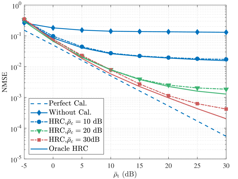
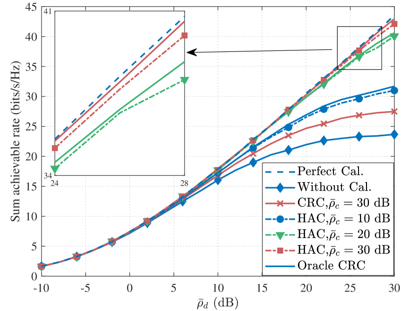
Fig. 8 demonstrates the NMSE of estimated uplink channel versus the SNR of the training signals for the channel estimation, where the SNR of calibration signals is set to dB, dB, and dB. It can be seen that the NMSE of the perfect calibration decreases with the increase of the training SNR, while the NMSE of the uncalibrated case almost remains constant. The NMSE of the channel estimation with the proposed HAC also decreases and gradually achieves floors with the training SNR increasing. The floor effect is caused by the estimation error of mismatch coefficients. When the SNR of calibration signals increases, the curves of the proposed HAC can approach the curve of the perfect calibration, which is because the estimation error of mismatch coefficients decreases. Further, since the NMSE of HAC is much less than the NMSE of the uncalibrated case, the proposed HAC can improve the system performance of the mmWave-HBF system, significantly.
IV-C Achievable Rate of Downlink Transmission
To further examine the efficacy of the reciprocity calibration in mmWave-HBF systems, we study the achievable rate of the downlink transmission. During the downlink transmission, the transmit analog beamforming is set to , and the receive analog beamforming is equal to , where is the first columns of , is the first columns of , and are obtained from the SVD of , i.e., . The digital precoding and the digital receiver are set to and , where and consist of the first columns of and , and can be obtained from the SVD of the equivalent downlink channel . Thus, based on the downlink transmission model (5), the sum achievable rate can be denoted as
| (44) |
where denotes the data stream number, and , denotes the -th entry of , and is the -row of .
The sum achievable rate of downlink transmission with the reciprocity calibration versus the downlink transmission SNR is illustrated in Fig. 8. From the figure, it can be observed that the curves of the systems with the perfect calibration, HAC, CRC, and without calibration achieve the same performance in the low SNR regime. This is because the impact of the noise is much larger than the reciprocity mismatch when the transmission SNR is small. In the high SNR regime, the achievable rate of the uncalibrated system converges to an upper bound, which is caused by multi-stream interference. Also, the achievable rate of the system applying HAC achieves the upper limit when the transmit SNR increases. For the perfectly calibrated system, the achievable rate linearly increases with the log function of the transmit SNR increasing. This is because the multi-stream interference can be completely mitigated by the HBF beamforming with perfect knowledge of mismatch coefficients. Further, we can also find that the achievable rate of HAC with dB is almost twice larger than that of the uncalibrated case. This result implies that the reciprocity calibration can significantly improve the system performance as expected. Besides, the achievable rate of the system using HAC is larger than that using CRC, which indicates the proposed HAC outperforms the CRC.
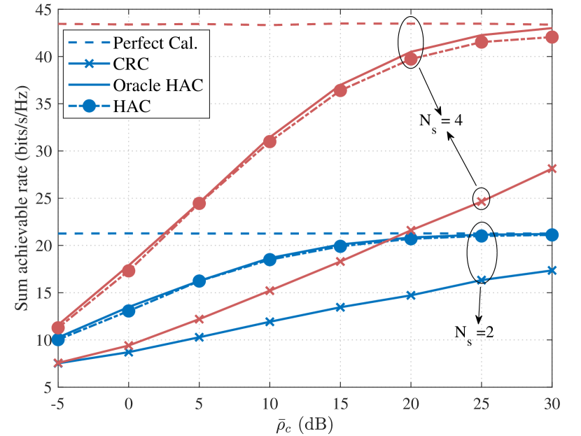
Fig. 10 demonstrates the sum achievable rate versus the SNR of the calibration signals, where the number of data streams is set to and , and the SNR of the downlink transmission signals is set to dB. It can be found that the sum achievable rate increases with the SNR of calibration signals increasing. This is because the estimation error decreases with the increase of the calibration SNR and the power of the interference decreases with the decrease of the estimation error of the mismatch coefficients. The gaps between the rates of the system using the proposed HAC and those of the perfectly calibrated systems are much smaller than the gaps between the rates of the system using CRC and those of the perfectly calibrated system. Further, when , the curve of HAC approaches the curve of the perfect calibration more quickly. This result indicates that the system transmitting more data streams requires higher calibration SNR to have the same performance loss.
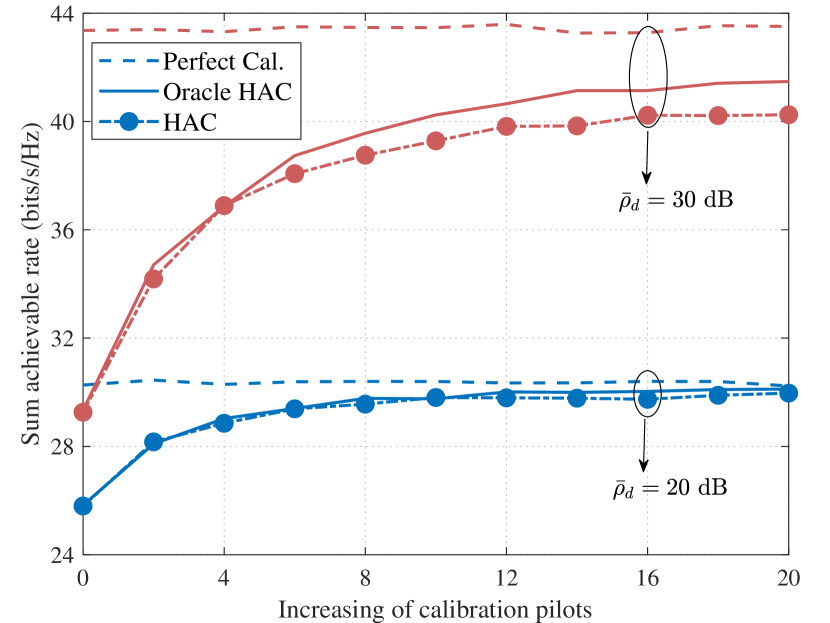
Finally, we examine the sum achievable rate versus the length of calibration pilots illustrated in Fig. 10, where the SNR of the downlink transmission signals is set to dB and dB, and the SNR of calibrations signals is set to dB. From the figure, it can be observed that the achievable rate increases with the length of calibration pilots increasing, which is because the estimation error of the mismatch coefficients decreases with the increase of the calibration pilots. Further, the system with higher transmit SNR requires smaller calibration errors to guarantee the same performance loss.
V Conclusion
In this paper, we have proposed a hierarchical-absolute reciprocity calibration for the mmWave-HBF system with the fully-connected phase shifter network. By proposing a specific beamforming design, the reciprocity calibration of the HBF system has been decoupled into the reciprocity calibration of digital RF chains and analog RF chains. Based on the decoupling, the entire reciprocity calibration problem of the HBF system has been equivalently decomposed into two subproblems corresponding to the reciprocity calibrations of digital and analog RF chains. Theoretical analysis has revealed that the overhead and computational complexity of the proposed HAC is much smaller than the conventional reciprocity calibration of HBF systems due to the decoupling. Further, based on the proposed calibration approach, we have derived the CRLB of the mismatch coefficients, which indicated that the estimation errors of the mismatch coefficients of digital and analog RF chains were independent, and the mismatch coefficients of receive digital chains could be estimated perfectly. Finally, simulation results have demonstrated that the proposed HAC significantly improved the system performance and outperformed the conventional calibration.
Appendix A Proof of Proposition 2
Based on the specific design of the digital/analog beamforming matrices, when , the received signal in (13) can be rewritten as
| (45) |
where , consists of the diagonal entries of , and is composed of the diagonal entries of . By stacking all -length signals into the matrix form, the received signals can be further denoted as
| (46) |
where , , , , .
Similarly, when , by substituting the designed beamforming matrices into (13), the received signal can be rewritten as
| (47) |
which indicates that signal received by the first receive digital RF chain is valid. By stacking all -length signals into matrix form, the received signal can be further denoted as
| (48) |
where , , , , , , and .
By substituting (46) and (48) into (14), the optimization problem can be rewritten as
| (49) |
From (49), it can be observed that the functions and are coupled to each other through the variables , , and . Fortunately, any vector parallel to the mismatch coefficient vector can be exploited to calibrate the reciprocity mismatch of digital RF chains. This fact indicates that the unknown variable in the function can be regarded as a scale factor of or . Similarly, since any vector parallel to the mismatch coefficient vector can be used to calibrate the reciprocity mismatch of analog RF chains, the unknown variable in the function can be also treated as a scale factor of or . Therefore, (49) can be equivalently written as
| (50) |
It is worth noting that the solutions to the problem (50) are also the solutions to the problem (49). Further, since and are independent of each other, the minimum sum of these two functions is equal to the sum of the minimum of each function, i.e., . Consequently, the problem (50) can be decoupled into two independent subproblems denoted as
| (51) |
Thus, Proposition 2 holds.
Appendix B Proof of Proposition 3
By substituting in (19) and into (15), the objective of the problem can be further denoted as
| (52) |
where consists of the second to the last row of , and . By defining , , and , can be rewritten into the matrix form denoted as
| (53) |
Then, can be equivalently transformed into
| (54) |
Since the objective of is the sum of two convex functions, is a convex problem without constraints. Thus, to solve , we take the partial derivative of with respect to as follows
| (55) |
By setting the derivative equal to zero, the solution to can be given by
| (56) |
where the condition holds when is a full column rank matrix.
Similarly, by taking the partial derivative of with respect to and setting the partial derivative to zero, we can obtain the solution to denoted as follows
| (57) |
where the condition holds when is full column rank. Thus, Proposition 3 holds.
References
- [1] Erik G. Larsson, Ove Edfors, Fredrik Tufvesson and Thomas L. Marzetta “Massive MIMO for next Generation Wireless Systems” In IEEE Commun. Mag. 52.2, 2014, pp. 186–195 DOI: 10.1109/MCOM.2014.6736761
- [2] Jose Flordelis et al. “Massive MIMO Performance—TDD Versus FDD: What Do Measurements Say?” In IEEE Trans. Wireless Commun. 17.4, 2018, pp. 2247–2261 DOI: 10.1109/TWC.2018.2790912
- [3] Chuanqiang Shan, Li Chen, Xiaohui Chen and Weidong Wang “A General Matched Filter Design for Reciprocity Calibration in Multiuser Massive MIMO Systems” In IEEE Trans. Veh. Technol. 67.9, 2018, pp. 8939–8943 DOI: 10.1109/TVT.2018.2839591
- [4] Rongjiang Nie et al. “Impact and Calibration of Nonlinear Reciprocity Mismatch in Massive MIMO Systems” In IEEE Trans. Wireless Commun. 20.10, 2021, pp. 6418–6435 DOI: 10.1109/TWC.2021.3073949
- [5] Wence Zhang et al. “Large-Scale Antenna Systems With UL/DL Hardware Mismatch: Achievable Rates Analysis and Calibration” In IEEE Trans. Commun. 63.4, 2015, pp. 1216–1229 DOI: 10.1109/TCOMM.2015.2395432
- [6] Hao Wei, Dongming Wang, Jiangzhou Wang and Xiaohu You “Impact of RF Mismatches on the Performance of Massive MIMO Systems with ZF Precoding” In Sci. China Inf. Sci. 59.2, 2016, pp. 1–14 DOI: 10.1007/s11432-015-5509-1
- [7] Orod Raeesi et al. “Performance Analysis of Multi-User Massive MIMO Downlink Under Channel Non-Reciprocity and Imperfect CSI” In IEEE Trans. Commun. 66.6, 2018, pp. 2456–2471 DOI: 10.1109/TCOMM.2018.2792017
- [8] Xiliang Luo “Multiuser Massive MIMO Performance With Calibration Errors” In IEEE Trans. Wirel. Commun. 15.7, 2016, pp. 4521–4534
- [9] Xiwen Jiang et al. “MIMO-TDD Reciprocity under Hardware Imbalances: Experimental Results” In IEEE Int. Conf. Commun., 2015, pp. 4949–4953 DOI: 10.1109/ICC.2015.7249107
- [10] De Mi et al. “Massive MIMO Performance With Imperfect Channel Reciprocity and Channel Estimation Error” In IEEE Trans. Commun. 65.9, 2017, pp. 3734–3749
- [11] K. Nishimori, K. Cho, Y. Takatori and T. Hori “Automatic Calibration Method Using Transmitting Signals of an Adaptive Array for TDD Systems” In IEEE Trans. Veh. Technol. 50.6, 2001, pp. 1636–1640 DOI: 10.1109/25.966592
- [12] A. Bourdoux, B. Come and N. Khaled “Non-Reciprocal Transceivers in OFDM/SDMA Systems: Impact and Mitigation” In Proc. IEEE Radio Wirel. Conf. (RAWCON) Boston, Massachusetts, USA: IEEE, 2003, pp. 183–186 DOI: 10.1109/RAWCON.2003.1227923
- [13] A. Benzin and G. Caire “Internal Self-Calibration Methods for Large Scale Array Transceiver Software-Defined Radios” In Proc. Int. ITG Workshop Smart Antennas (WSA), 2017, pp. 1–8
- [14] Xiliang Luo, Fuqian Yang and Hanyu Zhu “Massive MIMO Self-Calibration: Optimal Interconnection for Full Calibration” In IEEE Trans. Veh. Technol. 68.11, 2019, pp. 10357–10371 DOI: 10.1109/TVT.2019.2941544
- [15] Florian Kaltenberger, Haiyong Jiang, Maxime Guillaud and Raymond Knopp “Relative Channel Reciprocity Calibration in MIMO/TDD Systems” In Proc. Futur. Netw. Mob. Summit, 2010, pp. 1–10
- [16] M. Guillaud, D.T.M. Slock and R. Knopp “A Practical Method for Wireless Channel Reciprocity Exploitation through Relative Calibration” In Proc. 8th Int. Symp. Signal Process. Applic. (ISSPA) 1 Sydney, Australia: IEEE, 2005, pp. 403–406 DOI: 10.1109/ISSPA.2005.1580281
- [17] Mark Petermann et al. “Low-Complexity Calibration of Mutually Coupled Non-Reciprocal Multi-Antenna OFDM Transceivers” In Proc. 7th Int. Symp. Wireless Commun. Syst. York: IEEE, 2010, pp. 285–289 DOI: 10.1109/ISWCS.2010.5624277
- [18] Boris Kouassi, Irfan Ghauri and Luc Deneire “Estimation of Time-Domain Calibration Parameters to Restore MIMO-TDD Channel Reciprocity” In Proc. 7th Int. ICST Conf. Cogn. Radio Oriented Wirel. Networks Commun. Stockholm, Sweden: IEEE, 2012 DOI: 10.4108/icst.crowncom.2012.248472
- [19] Clayton Shepard et al. “Argos: Practical Many-Antenna Base Stations” In Proc. 18th Annu. Int. Conf. Mobile Comput. Networking (Mobicom) Istanbul, Turkey: ACM Press, 2012, pp. 53 DOI: 10.1145/2348543.2348553
- [20] Hao Wei et al. “Mutual Coupling Calibration for Multiuser Massive MIMO Systems” In IEEE Trans. Wireless Commun. 15.1, 2016, pp. 606–619 DOI: 10.1109/TWC.2015.2476467
- [21] Xiwen Jiang et al. “A Framework for Over-the-Air Reciprocity Calibration for TDD Massive MIMO Systems” In IEEE Trans. Wireless Commun. 17.9, 2018, pp. 5975–5990 DOI: 10.1109/TWC.2018.2853743
- [22] R. Rogalin et al. “Hardware-Impairment Compensation for Enabling Distributed Large-Scale MIMO” In Proc. 2013 Inf. Theory Appl. Work. (ITA) San Diego, CA: IEEE, 2013, pp. 1–10 DOI: 10.1109/ITA.2013.6502966
- [23] Liyan Su, Chenyang Yang, Gang Wang and Ming Lei “Retrieving Channel Reciprocity for Coordinated Multi-Point Transmission with Joint Processing” In IEEE Trans. Commun. 62.5, 2014, pp. 1541–1553 DOI: 10.1109/TCOMM.2014.031014.130367
- [24] Rongjiang Nie et al. “Relaying Systems With Reciprocity Mismatch: Impact Analysis and Calibration” In IEEE Trans. Commun. 68.7, 2020, pp. 4035–4049 DOI: 10.1109/TCOMM.2020.2982632
- [25] Andreas F. Molisch et al. “Hybrid Beamforming for Massive MIMO: A Survey” In IEEE Commun. Mag. 55.9, 2017, pp. 134–141 DOI: 10.1109/MCOM.2017.1600400
- [26] X. Wei, Y. Jiang, Q. Liu and X. Wang “Calibration of Phase Shifter Network for Hybrid Beamforming in mmWave Massive MIMO Systems” In IEEE Trans. Signal Process. 68, 2020, pp. 2302–2315
- [27] Xiwen Jiang and Florian Kaltenberger “Channel Reciprocity Calibration in TDD Hybrid Beamforming Massive MIMO Systems” In IEEE J. Sel. Topics Signal Process. 12.3, 2018, pp. 422–431 DOI: 10.1109/JSTSP.2018.2819118
- [28] Z. Guo, X. Wang and W. Heng “Millimeter-Wave Channel Estimation Based on 2-D Beamspace MUSIC Method” In IEEE Trans. Wireless Commun. 16.8, 2017, pp. 5384–5394 DOI: 10.1109/TWC.2017.2710049
- [29] Kiran Venugopal, Ahmed Alkhateeb, Nuria González Prelcic and Robert W. Heath “Channel Estimation for Hybrid Architecture-Based Wideband Millimeter Wave Systems” In IEEE J. Sel. Areas Commun. 35.9, 2017, pp. 1996–2009
- [30] Wei Zhang, Miaomiao Dong and Taejoon Kim “MMV-Based Sequential AoA and AoD Estimation for Millimeter Wave MIMO Channels” In IEEE Trans. Commun. 70.6, 2022, pp. 4063–4077
- [31] Xizixiang Wei, Yi Jiang, Xin Wang and Cong Shen “Tx-Rx Reciprocity Calibration for Hybrid Massive MIMO Systems” In IEEE Wireless Commun. Lett., 2021, pp. 1–1
- [32] Foad Sohrabi and Wei Yu “Hybrid Digital and Analog Beamforming Design for Large-Scale Antenna Arrays” In IEEE J. Sel. Topics Signal Process. 10.3, 2016, pp. 501–513
- [33] Xianghao Yu, Juei-Chin Shen, Jun Zhang and Khaled B. Letaief “Alternating Minimization Algorithms for Hybrid Precoding in Millimeter Wave MIMO Systems” In IEEE J. Sel. Topics Signal Process. 10.3, 2016, pp. 485–500
- [34] Tian Lin et al. “Hybrid Beamforming for Millimeter Wave Systems Using the MMSE Criterion” In IEEE Trans. Commun. 67.5, 2019, pp. 3693–3708
- [35] O.. Ayach et al. “Spatially Sparse Precoding in Millimeter Wave MIMO Systems” In IEEE Trans. Wireless Commun. 13.3, 2014, pp. 1499–1513 DOI: 10.1109/TWC.2014.011714.130846
- [36] Xian-Da Zhang “Matrix Analysis and Applications” Cambridge University Press, 2017, pp. 325–329
- [37] De Mi et al. “Self-Calibration for Massive MIMO with Channel Reciprocity and Channel Estimation Errors” In in Proc. IEEE Global Commun. Conf. (GLOBECOM) Abu Dhabi, United Arab Emirates: IEEE, 2018, pp. 1–7
- [38] De Mi et al. “Massive MIMO in Mobile Networks: Self-Calibration with Channel Estimation Error” In in Proc. ACM MobiArch 15th Workshop Mobility Evolving Internet Archit., MobiArch’20 New York, USA: Association for Computing Machinery, 2020, pp. 30–35
- [39] James C. Bezdek and Richard J. Hathaway “Convergence of Alternating Optimization” In Neural Parallel Sci. Comput. 11.4, 2003, pp. 351–368
- [40] Zai Yang, Lihua Xie and Cishen Zhang “Off-Grid Direction of Arrival Estimation Using Sparse Bayesian Inference” In IEEE Trans. Signal Process. 61.1, 2013, pp. 38–43
- [41] Biqing Qi, Wei Wang and Ben Wang “Off-Grid Compressive Channel Estimation for Mm-Wave Massive MIMO With Hybrid Precoding” In IEEE Commun. Lett. 23.1, 2019, pp. 108–111 DOI: 10.1109/LCOMM.2018.2878557
- [42] Steven M. Kay “Fundamentals of Statistical Signal Processing”, Prentice Hall Signal Processing Series Englewood Cliffs, N.J: Prentice-Hall PTR, 1993, pp. 45–47
References
- [43] Roger A. Horn and Zai Yang “Rank of a Hadamard Product” In Linear Algebra and its Applications 591, 2020, pp. 87–98 DOI: 10.1016/j.laa.2020.01.005
- [44] Steven M. Kay “Fundamentals of Statistical Signal Processing”, Prentice Hall Signal Processing Series Englewood Cliffs, N.J: Prentice-Hall PTR, 1993, pp. 45–47
labelnumberR#1
Supplementary Material for “Hierarchical-Absolute Reciprocity Calibration for Millimeter-wave Hybrid Beamforming Systems”
Li Chen, Rongjiang Nie, Yunfei Chen, and Weidong Wang
Some proofs are omitted in the main paper for readability, and we provide the missing content in this supplementary material for completeness.
Appendix C Proof of Lemma 1
To estimate the diagonal matrix , the objective of can be further denoted as
| (58) |
When are known during the -iteration, is a convex function corresponding to . Thus, can be estimated by taking the derivative of , and the solution to is given by
| (59) |
where .
Similarly, the diagonal entries of and can be estimated as
| (60) | |||
| (61) |
where , and . Thus, Lemma 1 holds.
Appendix D Proof of Proposition 4
We first derive the pilot requirement for calibrating the digital RF chains. According to (20), to guarantee a unique solution to , the matrix should have column rank, which is always satisfied when and . Similarly, based on (21), for computing , the matrix should have column rank, i.e., . Thus, the pilots of digital RF chain calibration should satisfy
| (62) |
Then, we derive the pilot requirement for calibrating the analog RF chains. To guarantee the unique solution to , must be full column rank, i.e.,
| (63) |
Since it is difficult to determine the krank of any matrices, we derive a sufficient condition to guarantee the above inequality to hold, which is denoted as
| (64) |
To guarantee the unique solution to during the iteration, must be full rank, i.e., . can be further expressed by the Hadamard product denoted as
| (65) |
According to [43, (10)], the rank of the Hadamard product is given by
| (66) |
As is artificially designed, we assume that . Further, because of , . Accordingly, we can obtain the inequality denoted as
| (67) |
Similarly, to guarantee the unique solution to during the iteration, the rank of must be . Since is artificially designed, we can obtain the following inequality denoted as
| (68) |
The solution to the inequalities consisting of (64), (67), and (68) is given by
| (69) |
Therefore, Proposition 4 holds.
Appendix E Proof of Lemma 2
We use to denote the received signal vector for estimating . The corresponding probability density function of is defined as . Then, the Fisher information matrix can be defined as [44]
| (70) |
In Section II-C, the received training signal consists of two independent parts and , i.e., , where is utilized to estimate and , and is used to estimate and . Thus, by dividing the vector into two independent parts, i.e., , the corresponding probability density function of can be further denoted as , where , , and denote the corresponding probability density functions of and . Then, based on (70), the Fisher information matrix can be further given by
| (71) |
where holds due to the independence between and as well as the independence between and , denotes the Fisher information matrix of , and denotes the Fisher information matrix of . Thus, Lemma 2 holds.
Appendix F Proof of Lemma 3
In Section II-C, and are estimated from the received signal and , respectively. According to Proposition 3, and are denoted as
| (72) |
Thus, similar to Lemma 2, we have due to the independence between and , where , and .
To derive the fishier information matrices, we first model the received signal . Based on (45) and (46), can be denoted as
| (73) |
where . Then, we have
| (74) |
As we set the first receive digital RF chain of the UE to be the reference, e.g., , is equal to the first row of , i.e., . This result indicates that is a deterministic signal without noises for computing . To derive the closed-form expression of , we regard computing as an asymptotic case of the estimation from the signal in white Gaussian noise with zero mean and zero variance. Thus, By using the vectorization of , (74) can be rewritten as
| (75) |
where each entry of is distributed as , and . Thus, is distributed as , where . Since and based on [44, (3.31)], the Fisher information matrix is given by
| (76) |
Further, to derive the closed-form expression of , we use the fact that . The received signal is distributed as , where . Further, since , the closed-form expression of can be given by
| (77) |
where , and the step holds by assuming that is orthogonal in the time domain and since . Thus, Lemma 3 holds.
Appendix G Proof of Lemma 4
In Section II-D, and are jointly estimated by using the received signal . According to (48), can be given by
| (78) |
which obeys complex Gaussian distribution, i.e., , where
| (79) |
We first derive the partial derivative of with the respect to , which is denoted as
| (80) |
where . Similarly, the partial derivative of with the respect to is denoted as
| (81) |
where , and , is the -the column of .
Appendix H Proof of Proposition 5
The partial derivative of the transformation function with respect to can be denoted as
| (83) |
Based on the definition of CRLB, we can obtain
| (84) |
where . By substituting (39) and (40) into (84), the CRLB of can be given by (41).