Heckerthoughts
1 Introduction
In 1987, Eric Horvitz, Greg Cooper, and I visited I.J. Good at Virginia Polytechnic and State University. The three of us were at a conference in Washington DC and made the short drive to see him. The primary reason we wanted to see him was not because he worked with Alan Turing to help win WWII by decoding encrypted messages from the Germans, although that certainly intrigued us. Rather, we wanted to see him because we had just finished reading his book “Good Thinking” [31], which summarized his life’s work in Probability and its Applications. We were delighted that he was willing to have lunch with us. We were young graduate students at Stanford working in Artificial Intelligence (AI), and were amazed that his thinking was so similar to ours, having worked decades before us and coming from such a seemingly different perspective not involving AI. We had lunch and talked about many topics of shared interest including Bayesian probability, graphical models, decision theory, AI (he was interested by then), how the brain works, and the nature of the universe. Before we knew it, it was dinner time. We took a brief stroll around the beautiful campus and sat down again for dinner and more discussion. Figure 1 is a photo taken just before we reluctantly departed.

This story is a fitting introduction this manuscript. Now having years to look back on my work, to boil it down to its essence, and to better appreciate its significance (if any) in the evolution of AI and Machine Learning (ML), I realized it was time to put my work in perspective, providing a roadmap to any who would like to explore it in more detail. After I had this realization, it occurred to me that this is what I.J. Good did in his book.
This manuscript is for those who want to understand basic concepts central to ML and AI, and to learn about early applications of these concepts. Ironically, after I finished writing this manuscript, I realized that a lot of the concepts that I included are missing in modern courses on ML. I hope this work will help to make up for these omissions. The presentation gets somewhat technical in parts, but I’ve tried to keep the math to the bare minimum to convey the fundamental concepts.
In addition to the technical presentations, I include stories about how the ideas came to be and the effects they have had. When I was a student in physics, I was given dry texts to read. In class, however, several of my physics professors would tell stories around the work, such as Einstein’s thinking that led to his general theory of relativity. Those stories fascinated me and really made the theory stick. So here, I do my best to present both the fundamental ideas and the stories behind them.
As for the title, “Heckerman Thinking” doesn’t have the same ring to it as that of Good’s book. I chose “Heckerthoughts,” because my rather odd last name has been humorous fodder for friends and colleagues for naming things related to me such as “Heckerperson,” “Heckertalk,” and “Heckerpaper”—you get the idea. Ironically, a distant relative of mine who connected with me via 23andMe is a genealogist, and discovered that my true last name is “Eckerman,” with my father’s ancestors coming from a region in Germany near the Ecker River. In any case, “Heckerthoughts” it is.
2 Uncertainty and AI’s transition to probability
In the early 1980, I joined the AI program at Stanford while also getting my M.D. degree. I actually went to medical school to learn how the brain works and was lucky to go to Stanford where AI—an arguably better way to study the workings of the brain—was flourishing. I immediately began taking courses in AI and had one big surprise. AI, of course, had to deal with uncertainty. When robots move, they are not completely certain about their position. When suggesting medical diagnoses, an expert system may not be certain about a diagnosis, even when all the evidence was in. The surprise was that I was told, very clearly, that probability was not a good measure of uncertainty. I was told that measures such as the Certainty Factor model [73, 11] were better. Just coming off of six years of training in physics, where fluency with probability was a must, and where the Bayesian interpretation was often mentioned (although not by name as I recall), I was taken aback by these statements.
Over the next half a dozen years or so, probability gradually became accepted by the AI community, and I’ve been given some credit for that. In this section, I will start with a clean and compelling argument for probability that has nothing to do with my work. Although everything in this argument was known by the time John McCarthy coined the term “Artificial Intelligence” in 1955, there was no email, Facebook, or Twitter to spread the word. Consequently, AI’s actual transition to probability was much more tortured. At the end of this next section, I discuss that transition and the role that I think I played.
2.1 The inevitability of probability
Let’s put aside the notion of probability for the moment. Rather, let’s focus on the important and frequent need to express one’s uncertainty about the truth of some proposition or, equivalently, the occurrence of some event. For example, I’m fairly sure that I don’t have COVID right now, but I am not certain. How do I tell you just how certain I am? Also, note that I am talking about my uncertainty, not anyone else’s. Uncertainty is subjective. What properties do we want this form of communication to have?
Property 1: A person’s uncertainty about the truth of some proposition can be expressed by a single (real) number. Let’s call it a degree of belief and use to denote the degree of belief that proposition is true. At the end of this section, we will discuss the process of putting a number on a degree of belief. An important point here is that a degree of belief is not expressed in a vacuum, but rather in the context of all sorts of information in the person’s head. We say that all degrees of belief are “conditional,” and write to denote a person’s degree of belief in given their background information . Another point is that, sometimes, we want to explicitly call out a specific proposition that a degree of belief is conditioned on. For example, I may want to express my degree of belief that I have COVID, given that I have no symptoms. I use to denote a degree of belief that proposition is true given that is true and given . In much of my past work, I explicitly mentioned , but this notation can get cumbersome. Going forward, I will exclude it.
Property 2: Suppose a person wants to express their belief about the proposition , which denotes the “AND” of proposition and proposition . One way to do this is to express their degree of belief directly. Another way to express their degrees of belief and , and then somehow combine them to yield . Property 2 says there is a function that combines and to yield . We write
A natural, albeit technical, assumption is that the function is continuous and monotonic increasing in both of its arguments.
Now let’s think about , the degree of belief that three propositions , , and are true. One way to do this is to decompose in terms of and , and then decompose the latter belief in terms of and :
Another way to do this is to decompose in terms of and , and then decompose in terms of and :
It follows that is associative:
| (1) |
Property 3: It’s often useful to relate the degree of belief in to the degree of belief about the negation of proposition , which I denote . So, another desirable property is that there is a function such that
That is, a degree of belief in and its negation move in (opposite) lock step. Another natural, albeit technical, assumption is that is continuous and monotonic.
Remarkably, it turns out that, if you accept Properties 1 through 3, a degree of belief must satisfy the following rules:
where and . These rules are precisely those of probability! Namely,
| (2) |
| (3) |
Cox [19] was the first to prove that properties 1 through 3 imply that a degree of belief must satisfy the rules of probability, although he used a slightly stronger technical assumptions for the functions and . The results here, which assume only continuity and monotonicity, are based on work by Aczel [1], who uses a set of mathematical tools known as functional equations to show that functions satisfying simple properties must have particular forms. Notable is his “Associativity Equation,” where he shows that any continuous, monotonic increasing, and associative function is isomorphic to the addition of numbers (see pages 256-267). This is a remarkable result, as it says that any such function can be implemented on a slide rule. It is a key step in proving the inevitability of probability from Equation 1 and the other properties.
Given these results, the term “probability” gets confusing quickly. Namely, a probability can be a long-run fraction in repeated experiments or a degree of belief, but obey the same syntactic rules. It’s tempting to call them both probabilities, but doing so obscures their very different semantics. To avoid this confusion, when the semantics are unclear from the text, I will refer to degrees of belief as Bayesian or subjective probabilities, and will refer to long-run fractions in repeated experiments as frequentist probabilities. I’ll use , , and , to refer to a degree of belief, frequentist probability, or one of the two, respectively.
One pet peeve of mine is that Bayesian thinking—using the rules of probability to govern degrees of belief—is often confused with Bayes rule, which follows directly from the syntactic product rule of probability (Equation 2). That is, Bayes rule can be applied equally well to Bayesian or frequentist probabilities. In this manuscript, I’ll try to eliminate this confusion by avoiding use of the phrase “Bayes rule” and instead refer to “the rules of probability” or sometimes more precisely “the product rule of probability.”
Thomas Bayes was possibly the first person known to apply the syntactic rules of probability to the semantics of degree of belief [6]. (I say “possibly,” because historical scholars disagree on this point.) Laplace definitively made this observation [55]. Note that Laplace and perhaps Bayes said only that the rules of probability could be applied to degrees of belief. They did not realize that, given Properties 1 through 3, this application was necessary.
One very practical problem is how to put a number on a degree of belief. A simple approach is based on the observation that people find it fairly easy to say that two propositions are equally likely. The approach is as follows. Imagine a simplified wheel of fortune having only two regions (shaded and not shaded), such as the one illustrated in Figure 2. Assuming everything about the wheel is symmetric (except for shading), the degree of belief that the wheel will stop in the shaded region is the fractional area of the wheel that is shaded (in this case, 0.3). (Of course, given that degrees of belief are subjective, a person is not forced to make this judgment about symmetry.) This wheel now provides a reference for measuring your degrees of belief for other events. For example, what is my probability that I currently have COVID? First, I ask myself the question: Is it more likely that I have COVID or that the wheel when spun will stop in the shaded region? If I think that it is more likely that I have COVID, then I imagine another wheel where the shaded region is larger. If I think that it is more likely that the wheel will stop in the shaded region, then I imagine another wheel where the shaded region is smaller. Now I repeat this process until I think that having COVID and the wheel stopping in the shaded region are about equally likely. At this point, my degree of belief that you have COVID is the percent area of the shaded area on the wheel.

In general, the process of measuring a degree of belief is commonly referred to as a belief assessment. The technique for assessment that I have just described is one of many available techniques discussed in the Management Science, Operations Research, and Psychology literature. One problem with belief assessment that is addressed in this literature is that of precision. Can someone really say that their degree of belief is and not ? In most cases, no. Nonetheless, in most cases, degrees of belief are used to make decisions (I’ll say a lot more about this in Section 3) and these decisions are typically not sensitive to small variations in assessments. Well-established practices of sensitivity analysis help one to know when additional precision is unnecessary (e.g., [47]). Alternatively, a person can reason with upper and lower bounds on degrees of belief [31]. Another problem with probability assessment is that of accuracy. For example, recent experiences or the way a question is phrased can lead to assessments that do not reflect a person’s true beliefs [78]. Methods for improving accuracy can be found in the decision-analysis literature (e.g., [74]).
Finally, let’s consider frequentist probabilities and how they are related to degrees of belief. As we’ve just seen, a similarity is that both semantics are governed by the rules of probability. And, of course, there are differences. For example, assessing a degree of belief does not require repeated trials, whereas estimating a frequentist probability does. Consider an old-fashioned thumbtack—one with a round, flat head (Figure 3). If the thumbtack is thrown up in the air, it will come to rest either on its point and an edge of the head (heads) or lying on its head with point up (tails). In the Bayesian framework, a person can look at the thumbtack and assess their degree of belief that it will land heads on a toss. In the frequentist approach, we assert that there is some unknown frequentist probability of heads, (heads), such that the thumbtack will land heads on any toss with the same degree of belief. (Getting heads is said to be independent and identically distributed.) The connection? This degree of belief must be equal to (heads).

It turns out that the Bayesian and frequentist frameworks are fully compatible. If a person’s beliefs about a series of flips of arbitrary length has the property that any two sequences of the same length and the same number of heads and tails are judged to be equally likely, then the degrees of belief assigned to those outcomes are the same as the degrees of belief assigned to the outcomes in a situation where there exists an unknown frequentist probability that is equal to the degree of belief of heads on every flip. This result was first proven by de Finetti and generalizations of it followed [45]. In short, the frequentist framework can exist within the Bayesian framework. Ironically, despite this compatibility, Bayesians and frequentists—people who work exclusively within the Bayesian and frequentist frameworks, respectively—have been at odds with each other for many decades. The good news is that there is no need to choose—we can embrace both. And the battles seem to be subsiding.
2.2 Independence and graphical models
In the AI community, before 1985, a common argument made against the use of probability to reason about uncertainty was that general probabilistic inference was computationally intractable [73, 11]. For example, the number of combinations of binary variables is , and no human could assess that many degrees of belief or reason about them when is more than a dozen or so. The only alternative, it was argued, was to make incorrect assumptions of conditional independence. For example, when building an expert system to diagnose medical diseases, the builder could make the incorrect assumption that all symptoms are mutually independent given the true disease—the so called, “naive Bayes assumption.”
What the community missed was the fact that there were representations of conditional independence that were ideal for the task of representing uncertainty. They were graphical and hence easy to read and write and would accommodate assertions of conditional independence that were tailored to the task at hand.
In this manuscript, I will focus on the most used probabilistic graphical model, the directed acyclic graphical model, or DAG model. The model was first described by Sewell Wright in 1921 [83] and advanced by many researchers including I.J. Good [31].
To better understand DAG models, we should now move beyond the simple notion of a proposition to talk about a variable—a collection of mutually exclusive and exhaustive values (sometimes called “states”). I will typically denote a variable by an upper-case, potentially indexed letter (e.g., , and a value of a corresponding variable by that same letter in lower case (e.g., ). To denote a set of variables, I will use a bold-face upper-case letter (e.g., ), and will use a corresponding bold-face lower-case letter (e.g., ) to denote a value for each variable in a given set. When showing specific examples, I will sometimes give variables understandable names and denote them in typewriter font—for example, Age. To denote a probability distribution over , where has a finite number of values, I will use . In addition, I will use this same term to denote a probability for a value of . Whether the mention is a distribution or a single probability should be clear from context. Similarly, if is a continuous variable, then I will use to refer to ’s probability density function or the density at a given point.
DAG models can represent either Bayesian or frequentist probabilities. So, to start, let’s talk about them generically. Suppose we have a problem domain consisting of a set of variables . A DAG model for consists of (1) a DAG structure that encodes a set of conditional independence assertions about variables in , and (2) a set of local probability distributions, one associated with each variable. Together, these components define a probability distribution for , sometimes called a joint probability distribution. The nodes in the graph are in one-to-one correspondence with the variables . I use to denote both the variable and its corresponding node, and to denote the parents of node in the graph as well as the variables corresponding to those parents. The lack of possible arcs in the graph encode conditional independencies. To understand these independencies, let’s fix the ordering of nodes in the graph to be . This ordering is not necessary, but it keeps things simple. Because the graph is acyclic, it is possible to describe the parents of as a subset of the nodes . Given this description, the graph states the following conditional independencies:
| (4) |
Note that other conditional independencies can be derived from these assertions. Now, from (a generalization of) the product rule of probability, we can write
| (5) |
Combining Equations 4 and 5, we obtain
| (6) |
Consequently, the conditional independencies implied by the graph combined with the local probability distributions , determine the joint probability distribution for .
One other note about the acyclicity of these graphs: Such acyclicity has been criticized due to its lack of applicability in many situations, such as when there is bi-directional cause and effect. That said, if a model is built that includes the representation of time, where the observation of a quantity over time is represented with multiple variables, then most criticism disappears. Also, notably, Sewall Wright and others have considered atemporal graph models with cycles.
In Section 4, we will see how DAG models can be constructed for frequentist probabilities. Here, let’s return to the state of AI in the 1980s and consider how to create a DAG model for degrees of belief. Such models became known as Bayesian networks. After that, we’ll look at how these models can make reasoning with uncertainty computationally efficient.
To be concrete, let us build a simple Bayesian network for the task of detecting credit-card fraud. (Of course, in practice, there is an individual, typically an expert, who provides the knowledge that goes into the Bayesian network. Here, I’ll simply use “us” and “we”.) We begin by determining the variables to include in the model. One possible choice of variables for our problem is whether or not there is fraud (Fraud or ), whether or not there was a gas purchase in the last 24 hours (Gas or ), whether or not there was a jewelry purchase in the last hour (Jewelry or ), the age of the cardholder (Age or ), and the sex (at birth) of the cardholder (Sex or ). The values of these variables are shown in Figure 4.
This initial task is not always straightforward. As part of this task we should (1) correctly identify the goals of modeling (e.g., prediction versus decision making), (2) identify many possible findings that may be relevant to the problem, (3) determine what subset of those findings is worthwhile to model, and (4) organize the findings into variables having mutually exclusive and collectively exhaustive values. Difficulties here are not unique to modeling with Bayesian networks, but rather are common to most tasks. Although solutions are not always simple, some guidance is offered by decision analysts (e.g., citeBlueBook).
In the next phase of Bayesian-network construction, we build a directed acyclic graph that encodes our assertions of conditional independence. One approach for doing so is to choose an ordering on the variables, , and, for each , determine the subset of such that Equation 4 holds. In our example, using the ordering , let’s assert the following:
| (7) | |||||
| (8) | |||||
| (9) | |||||
| (10) |
These assertions yield the structure shown in Figure 4.

This approach has a serious drawback. If we choose the variable order carelessly, the resulting network structure may fail to reveal many conditional independencies among the variables. For example, if we construct a Bayesian network for the fraud problem using the ordering , we obtain a fully connected network structure. In the worst case, we must explore variable orderings to find the best one.
Fortunately, there is another technique for constructing Bayesian networks that does not require an ordering. The approach is based on two observations: (1) people can often readily assert causal relationships among variables, and (2) causal relationships typically reveal a full set of conditional independence assertions. So, to construct the graph structure of Bayesian network for a given set of variables, we can simply draw arcs from cause variables to their immediate effects. In almost all cases, doing so results in a network structure that satisfies the definition of Equation 6. For example, given the assertion that Fraud is a direct cause of Gas, the assertion that Fraud, Age, and Sex are direct causes of Jewelry, and the assertion that there are no other causes among these variables, we obtain the network structure in Figure 4.
In the next section, we will explore causality in detail. Here, it suffices to say that the human ability to naturally think in terms of cause and effect is in large part responsible for the success of the DAG model as a representation in AI systems (see Section 3).
In the final step of constructing a Bayesian network, we assess the local probability distributions . In our fraud example, where all variables are discrete, we assess one distribution for for every set of values for . Example distributions are shown in Figure 4. Although we have described these construction steps as a simple sequence, they are often intermingled in practice. For example, judgments of conditional independence and/or cause and effect can influence problem formulation. Also, assessments of probability can lead to changes in the network structure.
One final note: In some situations, a child can be a deterministic function of its parents. We can still be uncertain about the value of such a node, because we can be uncertain about the values of its parents. Given the values of its parents, however, the value of the child is determined with certainty. In those situations, I will draw the child node with a double oval. We will see an example of this situation when we consider influence diagrams.
Let’s now turn to how we can use this model to reason under uncertainty. In this case, we may want to infer the Bayesian probability of fraud, given observations of the other variables. This probability is not stored directly in the model and hence needs to be computed using the rules of probability. In general, the computation of a probability of interest given a model is known as probabilistic inference. This discussion on inference applies equally well to frequentist probabilities, so we can talk about both at the same time.
Because a DAG model for determines a joint probability distribution for , we can—in principle—use the model to compute any probability over the its variables. As an example, let’s compute the probability of fraud given observations of the other variables. Using the rules of probability, we have
| (11) |
For problems with many variables, however, this direct approach is computationally slow. Fortunately, we can use the conditional independencies encoded in the DAG, Equation 7, to make this computation more efficient. Equation 11 becomes
Many algorithms that exploit conditional independence in DAG models to speed up inference have been developed (see the annual proceedings of The Conference on Uncertainty in Artificial Intelligence—UAI). In some cases, however, inference in a domain remains intractable. In such cases, techniques have been developed that approximate results efficiently—for example, [27, 50].
2.3 AI’s transition to probability
The representation and use of conditional independence makes reasoning under uncertainty practical for a wide variety of tasks and, in hindsight, is largely responsible for AI’s transition to the use of probability for representing uncertainty. In this section, I highlight some key steps in the actual transition and the role I think I played in it.
In the late 1970s and early 1980s, multiple alternatives to probability were described, including Dempster–Shafer Theory and Fuzzy Logic. As my PhD advisor was Ted Shortliffe, my greatest exposure was to the Certainty Factor model, which he had developed for use in expert systems for medical diagnosis such as MYCIN and EMYCIN [73, 11]. The expert systems consisted of IF–THEN rules, which could be combined together in parallel or series, effectively forming a directed graph. Figure 5 shows a simple made-up example for diagnosing infection. An arc from node to corresponds to the rule IF THEN , where and are propositions that typically correspond to evidence and a hypothesis, respectively. An example of series combination is Sore throat Throat inflamed Infection. An example of parallel combination is Sore throat Throat inflamed Hoarse. Importantly, the semantics of the graph associated with a Certainty Factor model is different from that of the DAG model we have been considering. I use dashed lines for the former graph to highlight this difference. In the Certainty Factor model, arc direction goes from evidence (typically observed) to hypothesis (typically unobserved). In contrast, in a DAG model, arc direction typically goes from cause to effect. For some problems, each hypothesis in the model is a cause of the corresponding evidence, so that every arc in the Certainty Factor model and DAG model will point in the opposite direction. There are many instances, however, where this relationship does not hold.

Associated with each rule is a certainty factor , which was intended to quantify the degree to which changes the belief in . CFs range from -1 to 1. A CF of 1 corresponds to complete confirmation of ; a CF of -1 corresponds to complete disconfirmation of ; and a CF of 0 leaves the degree of belief of unchanged. In particular, a CF was not intended to represent an absolute degree of belief in given . The Certainty Factor model offers functions that combine these CFs when used in series and parallel. As a result, the model can infer a net increase or decrease in the degree of belief for a target hypothesis (Infection in this example), given multiple pieces of evidence. A list of properties or “desiderata” that these functions should obey were described.
One day in early 1985, as a teaching assistant for one of Ted’s medical informatics courses, I was listening to his explanation of the model. It occurred to me that CFs may simply be a transformation of probabilistic quantities. A simple candidate in my mind was the likelihood ratio . From the rules of probability, we have
| (12) | |||||
where and are the prior and posterior odds of , respectively. That is, the posterior odds of are just the product of the likelihood ratio and the prior odds of . (I.J. Good [31] wrote extensively about the logarithm of the likelihood ratio, known as the weight of evidence.) One catch was that the likelihood ratio ranges from 0 to infinity, but that was easy to fix: simply use a monotonic transformation to map the likelihood ratio to .
That night, I went home and gave the mapping a try. It satisfied the desiderata and closely matched the series and parallel combination functions in the Certainty Factor model. Even more important, the correspondence revealed that the Certainty Factor model facilitated the expression of conditional independence assertions that were less extreme than the naive-Bayes assumption. (In the example in Figure 5, the resulting conditional independencies can be identified by reversing the arcs in the figure and interpreting the result as a DAG model.) Given my proclivity for probability, I was excited and wrote up the result [33] [arXiv:1304.3419].
The work got an interesting mix of reactions. I was particularly nervous about what Ted would say about it, but he was very gracious. When he saw the result, he was very interested and gave me a set of papers to read to help me structure my thinking and prepare a publication. When I presented the work at the first UAI meeting that summer, it got a surprisingly good reception. At the time, the debate about probability as a measure of uncertainty was in full swing, having been ignited by Judea Pearl and Peter Cheeseman at the previous year’s AAAI Conference. Those in the probability camp welcomed the work. Ross Shachter and Jack Breese were perhaps the most surprised that someone from Stanford, the home of the Certainty Factor model, would be presenting such a result. We met for the first time there and have been friends and collaborators ever since.
I should note that there is an interesting connection between the Certainty Factor model and the modern reincarnation of the DAG model. In 1978, Dick Duda and Peter Hart created a variant of the Certainty Factor model for PROSPECTOR, a computer-based consultation system for mineral exploration [21]. Peter Hart went on to work at Stanford Research Institute, where he met Ron Howard and Jim Matheson. Ron and Jim saw this model and were inspired to create influence diagrams, an extension of DAG models that we discuss in the next section. After that, Judea Pearl heard Ron Howard talk about influence diagrams and began work his on DAG models [63].
For me, the next question to answer in AI’s transition to probability was the following: Is a monotonic transform of the likelihood ratio the only measure of a belief update? Over the next year, I took Ted’s desiderata, converted them to a series of functional equations (after learning about what Cox did with degrees of belief), and answered the question: a monotonic transform of the likelihood ratio is the only quantity satisfying these desiderata [34] [arXiv:1304.3091]. The support for probability was increasing. That said, critics were still in the majority.
The key remaining criticism of probability was that no one had built a successful probabilistic expert system. In 1984, that was about to change. Bharat Nathwani, a successful surgical pathologist from USC, visited Ted Shortliffe and several of students with the idea of building an expert system to aid surgical pathologists in the diagnosis of disease. The idea was straightforward: a surgical pathologist would look at one or more slides of tissue from a patient under the microscope, identify values for features such as the color or size of cells, report them to an expert system, and get back a list of possible diseases ordered by how likely they were given what was seen. Eric Horvitz and I were in that group of students and jumped at the chance. Over the next year, we built the first version of a probabilistic expert system for the diagnosis of lymph-node pathology, called Pathfinder. Even though we knowingly made the inaccurate assumption that features were mutually independent given disease, the system worked well—so well, that Bharat, Eric, and I started Intellipath, a company that would build expert systems for the diagnosis of all tissue types.
By now it was mid-1985, and fully appreciating Bayesian networks, I wanted to use the representation to incorporate important conditional dependencies among features. But there was a big catch: Bharat and I wanted to extend Pathfinder to include over 60 diseases and over 100 features. Even if we assumed features were mutually independent given disease, Bharat would have to assess almost ten thousand probabilities. So, over the next year I developed two techniques that made the construction of Bayesian networks for medical diagnosis in large domains easier and more efficient. This work became the focus of my PhD dissertation [44] [arXiv:1911.06263].
Before describing these techniques, I should note that diagnosis of disease in surgical pathology is well suited to the assumption that diseases are mutually exclusive. In particular, it is certainly possible for a patient to have two or more diseases, but these diseases are almost always spatially separated and easily identified as separate diseases. Both techniques make strong use of this assumption. In addition, both techniques make use of the following point. Let and denote two diseases, let denote some feature (e.g., cell size), and suppose that for each value of . From the rules of probability, we see that the ratio of disease priors and posteriors is the same:
| (13) |
In words, does not differentiate between the two diseases. It turns out that surgical pathologists (and experts in other fields) find it easier to think about whether differentiates diseases and , than think about whether . Comparing Equations 12 and 13, another way to think about this situation is that the observation , for any value , is a null belief update for , under the assumption that only and are possible.
The first technique was inspired by my discussions with Bharat about how he related findings to disease. He found it difficult to think about how a finding differentiated among all diseases. Rather, he liked to think about pairs of diseases and, for each pair, which of the many findings differentiated them. So, I developed the similarity graph, both an abstract concept and a graphical user interface, to allow him to do just that. An example for the simpler task of diagnosing five diseases that cause sore throat is shown in Figure 6. Each of the five diseases, which we assume to be mutually exclusive for purposes of presentation, correspond to a node in the similarity graph. An undirected edge between two diseases denotes that the expert is comfortable thinking about what features differentiate them. Note that every disease in the graph must border at least one edge, because otherwise some diseases could not be differentiated. After drawing the similarity graph, the expert can then click on one of the edges (in the small oval on the edge) and draw a local Bayesian network structure, a Bayesian network structure that includes the findings useful for differentiating the two diseases and the conditional independencies among these findings. Local structures for different disease pairs need not contain the same findings nor the same assertions of independence. So, unlike an ordinary Bayesian network structure, the technique allows for the specification of asymmetric conditional independencies. In my dissertation, I showed how the collection of local structures can be combined automatically to form a coherent (ordinary) Bayesian network structure for the entire domain. In addition, I showed how probability assessments for the local networks can automatically populate the distributions for this whole-domain structure [44] [arXiv:1911.06263]. The mathematics is interesting (see Chapter 3 and [24] [arXiv:1611.02126]). I called the similarity graph combined with the collection of local Bayesian networks a Probabilistic Similarity Network.


The second technique I developed made probability assessment even easier and more efficient than assessment within local structures. The technique uses a visual structure known as a partition. An example, again for the task of diagnosing sore throat, is shown in Figure 8. The box on the left shows a finding to be assessed (Palatal spots) along with the values for that finding. Each of the other boxes (in this example, there are two of them) contain diseases that are not differentiated by the finding. To construct this partition, the expert first groups diseases into boxes, and then, for each box, assesses a single probability distribution for the finding given any disease in the box. By Equation 13, there is only one distribution for each box. This technique generalizes easily to the case where the probabilities depend on other findings.

Using these techniques, Bharat and I built the extended version of Pathfinder in a relatively short amount of time and showed that its probabilistic diagnoses were accurate. Bharat, Eric, and I then used these same techniques to build many more expert systems for Intellipath. Then, on one sunny day in 1986 at Stanford, while Eric and I were riding our bikes from one class to the next, he said, “Let’s start a company to build expert systems for any diagnostic problem.” We agreed that Jack Breese should join the venture, and the company Knowledge Industries was born. Over the next several years, both Intellipath and Knowledge Industries continued to produce successful probabilistic expert systems based on Bayesian networks. With these results and the successful work of many others mostly in the UAI community, AI was fully embracing probability.
As luck would have it, these efforts brought Eric, Jack, and me to Microsoft. While finishing my Ph.D. and M.D., I got accepted as an assistant professor at UCLA—my dream job. Two weeks after finishing, I got a call from Nathan Myhrvold, a friend of mine from high school. He asked that we meet, ostensibly to catch up, and invited me to join him at Spago, a fancy restaurant in Beverly Hills (which seemed a bit odd). When I arrived, he told me about his work at Yale with Steven Hawking and his rise to vice-president at Microsoft having overseen version 2 of Windows. He then popped the question: “I read your dissertation and want you to come to Microsoft to apply your work to problems there.” Having just landed my dream job, I said, “No way, but you can buy Knowledge Industries.” Several months later, he did just that—an acqui-hire of Jack, Eric, and me.
3 Decision making and causal reasoning
Much of the work I did at Microsoft involved methods for decision making and its close cousin, causal reasoning. In this section, I introduce some basic concepts in these areas. In the following section, I cover some of my work in detail.
3.1 Decision theory, influence diagrams, and decision trees
Using probabilities to be precise about one’s uncertainties is important. It allows us to be precise in communicating our uncertainties to others. It also helps us make good decisions. To the second point, decision theory, developed in the middle of the twentieth century, provides a formal recipe for how to use subjective probability to make decisions. By the way, please don’t let the phrase “decision theory” scare you. As you will see, it is an extremely simple and intuitive theory—in essence, it is just common sense made precise.
Let’s start with an example to introduce the basics. Suppose we are the decision maker (so I don’t have to keep saying “decision maker”) and are deciding whether to have a party outdoors or indoors on a given day where the weather can be sunny or rainy. We can depict this decision problem using a graphical model known as an influence diagram, introduced by Ron Howard, my PhD advisor, and Jim Matheson [48]. The influence diagram for this party problem is shown in Figure 9.

In general, an influence diagram always contains three types of nodes, corresponding to three types of variables. Each type of variable, like any other variable, has a set of mutually exclusive values. In our example, there is one node/variable of each type. The square node Location corresponds to a decision variable. Each value of a decision variable corresponds to a possible action or alternative—in this example, indoors and outdoors. Other names that have been used for the value of a decision variable include “act” and “intervention.” The oval node Weather corresponds to an uncertainty variable (the type of variable seen in DAG models). In this example, let’s suppose this variable has only two relevant values: sunny or rainy. Finally, every influence diagram contains exactly one deterministic outcome node corresponding to the outcome variable. The values of the outcome variable correspond to all possible outcomes—that is, all combinations of alternatives and possible values of the uncertainty variables. In this example, the possible outcomes are (1) an outdoor sunny party, (2) an outdoor rainy party, (3) an indoor sunny party, and (4) an indoor rainy party.
An influence diagram can include multiple decision nodes, and can represent observations of uncertainty nodes interleaved with the making of individual decisions. The latter capability is important to the process of making real-world decisions, but is not central to the connection between decision making and causal reasoning. Consequently, to keep this presentation simple, I will assume that all decisions are made up front, before any uncertainty nodes are observed. For details on interleaving observations with decisions, see the discussion of “informational arcs” in [48].
As in a DAG model, the lack of arcs pointing to uncertainty variables encode assertions of conditional independence. In particular, given an ordering over decision and uncertainty variables, Equation 4 holds for each uncertainty variable, but now parent variables can include decision variables. Also, based on our assumption that decisions are made up front, the decision variables appear first in the variable ordering. In our party problem, the lack of an arc from Location to Weather corresponds to the assertion that the weather does not depend on our decision about the location of the party. Also as in a DAG model, an uncertainty variable in an influence diagram is associated with a local (subjective) probability distribution for each set of values of the variable’s parents. In our example, Weather has no parents, so this variable has only one distribution that encodes our prior beliefs that it will be rainy or sunny. Together, the assertions of independence and the local probability distributions define a joint distribution for the uncertainty variables conditioned on all possible alternatives.
The single outcome variable in an influence diagram encodes our preferences for the various outcomes. In particular, associated with each possible outcome is a number known as a utility. The larger the number, the more desirable the outcome. Utilities range between 0 and 1 (we will see why in a moment). That said, if the utilities are transformed linearly, the choice of the best alternative remains the same.
Decision theory says the decision maker should choose the alternative with the highest expected utility, where expectation is taken with respect to the decision maker’s joint distribution over uncertainty variables given each of the possible alternatives. In the party problem, expectation is taken with respect to (weather), which we assert does not depend on party location. Based on the utilities in Figure 9, the expected utility of the outdoor location is 0.7; the expected utility of the indoor location is 0.8; so, we should choose the indoor alternative. This principle is generally known as the principle of maximum expected utility or MEU principle.
Decision problems can also be represented with another type of graphical model known as a decision tree. This graphical model should not be confused with the “decision tree” used in the machine-learning community. Unfortunately, the two communities chose the same name for these rather different representations. When I use the term “decision tree,” I will make it clear which one I am talking about. Figure 10a shows the party problem depicted as a decision tree.

As in the influence diagram, a square node represents a decision variable, but now the variable’s values are drawn as edges emerging from the node. To the right of the decision variable come the uncertainty variables and possibly additional decision variables. In this case, there is just one uncertainty variable and no additional decision variables. Finally, utilities of the various outcomes are shown at the far right of the decision tree. Note that, in this case, the decision tree can be simplified, because the utility of the indoor location does not depend on the weather. The simplified decision tree is shown in Figure 10b.
When I first learned of influence diagrams (and decision trees) and the MEU principle, two questions immediately came up in my mind: What are these mysterious utilities? And what justifies the use of the MEU principle to choose the best alternative? In 1948, von Neumann and Morgenstern provided a very elegant answer to both questions. In a manner similar to Cox, von Neumann and Morgenstern introduced several properties that, if followed by a decision maker, define utilities and imply the MEU principle. Here, I’ll present a slightly different version of their argument given by my PhD advisor, Ron Howard [46]. I’ll use decision trees to present his argument and assume the rules of probability are in force.
Property 1 (orderability): Given any two outcomes, and , a decision maker can say whether they prefer to , prefer to , or are indifferent between the two—which I will write , , and , respectively. In addition, given any three outcomes , , and , if and , then . That is, preferences are transitive. If preferences were not transitive, a decision maker could be taken advantage of. For example, if they have the non-transitive preferences , , and , then they would pay money to get rather than , and again pay money to get rather than , and again to get rather than . So, they started and ended up with , but with less money. This observation illustrates an important point about this property and the other properties that we will consider. Namely, the properties are “normative” or “prescriptive”—that is, properties that a decision maker should follow. It is well known, however, that people often do not follow these properties when making real decisions [78]. Such decision making is sometimes referred to as “descriptive.” Unfortunately, people’s descriptive behavior have taken advantage of—for example, with unscrupulous forms of advertising.
Property 2 (continuity): Suppose there are three outcomes , , and , such that the decision maker has the preferences . Then the decision maker has some probability (with ) such that they are indifferent between getting for certain and getting a chance at the better versus worse outcome with probability . The situation is shown in the decision problem of Figure 11. As is the case with probability assessment in general, it is impossible in practice to assess with infinite precision, and such imprecision can be managed with sensitivity analysis.

Now consider the rather general decision problem shown in Figure 12a. Here, there are two alternatives and, for each alternative, a set of possible outcomes that will occur with the probabilities shown. As we will see, this decision problem is sufficiently general to make the argument. Given this decision problem, the first task of the decision maker is to identify the best and worst outcome, again denoted and , respectively. Then, for each possible outcome, the decision maker uses the continuity property to construct an equally preferred chance at getting the best versus worst outcome. The following property says that the decision maker can substitute this chance for the original outcome in the original decision problem, yielding the equivalent decision problem in Figure 12b.

Property 3 (substitutability): If a decision maker is indifferent between two alternatives in one decision problem, then they can substitute one for the other in another decision problem.
The resulting decision problem is simply a set of chances at the best versus worst outcome. The next property says that the decision maker can collapse these chances into one chance at the best versus worst outcome using the rules or probability.
Property 4 (decomposability): Given multiple chances at outcome versus with probabilities , the decision maker should equally prefer this situation to a single chance at outcome versus with probability . Ron calls this property the “no fun in gambling” property.
Given this property, the decision maker now has the equivalent decision problem shown in Figure 12c. The final property describes how the decision maker should make this decision.
Property 5 (monotonicity): Given two alternatives and between a chance at two outcomes , the decision maker should prefer the alternative if and only if the probability of getting in is higher than the probability of getting in .
Applying this property to the decision problem in Figure 12c yields the MEU principle, where the utility of an outcome is the probability of the chance at outcome versus . In addition, given the substitutability and decomposability properties, the decision problem in Figure 12a is sufficiently general to address any decision problem with two alternatives. Finally, there is a straightforward generalization of this argument to a decision problem with any number of alternatives.
In essence, these properties allow a decision maker to boil down any decision problem into a series of simple decision problems like the one in Figure 11. Note that this simple decision problem has the same form as the party problem. In the party problem, the decision maker is asked to assess utilities and apply the MEU principle to choose. The clever trick from von Neumann and Morgenstern is to recast this problem into one of choosing a probability of sunny that makes the alternatives outdoors and indoors equally preferable.
When I first saw this argument, I thought to myself, “This is the most elegant and practical application of math I have ever seen.” Both the assumptions and the proof of the MEU principle are simple, and the result is a tool that just about anyone can use to improve their decision making. This realization came to mind because my father was a high school math teacher and was always looking for practical applications of math to show his students. By the time I saw this proof, he had already retired, but nevertheless, we were both excited to discuss it.
To close this section, it’s worthwhile to comment on the two rather different graphical models for decision problems. The decision tree more naturally depicts the flow of time and the display of probabilities and utilities. Also, it allows the explicit depiction of any asymmetries in a decision problem, as we see in our example. In contrast, an influence diagram is typically more compact and, as mentioned, enables the explicit representation of probabilistic independencies. We will see examples of this benefit later. Given these tradeoffs, both representations are still in use.
3.2 Proper scoring rules
There is a special class of utility that is worth mentioning—namely, proper scoring rules. To motivate this class of utility, imagine you operate a company that invests is new and upcoming businesses. You are constantly making high-stakes decisions and sometimes need probabilities (or probability densities) from experts that various possible outcomes will occur, such as whether a particular piece of legislation in Washington is going to pass. You have access to experts, and want to be sure that the probabilities you get from them are “honest.” One way to do this is to frame the expert as a decision maker who is deciding what distribution to report over some variable , and then receiving a utility for that report based on the value of that is eventually observed. The utility they receive should be a function of (1) every possible observed value of and (2) the expert’s reported distribution for every possible value of . Let’s denote this utility function as . For the reported probability distribution to be honest, we want the expert’s expected utility to be a maximum when is equal to the expert’s actual probability distribution . That is, we want to be a maximum when . (Here, I am using generally—it can be a sum when is discrete.) When this condition holds, is said to be a proper scoring rule.
One proper scoring rule is the log scoring rule: —that is, is the logarithm of where is the value of that is actually observed. It is easy to check that utility is maximized when . What is rather remarkable, however, is that the log scoring rule is the only proper scoring rule (up to linear transformation) when (1) takes on three or more states, (2) is local in the sense that it only depends on at the observed value of , and (3) certain regularity conditions hold [7, 8]. The concept of a proper scoring rule will come in handy in Section 4.1, where we consider learning graphical models from data.
3.3 Correlation versus causation and a definition of causality
It’s tempting to sum up the difference between a purely probabilistic DAG model and an influence diagram by viewing the latter as merely the former with decisions and utilities “tacked on.” Nonetheless, there is something fundamentally different about them. In particular, an influence diagram can express causal relationships among its variables, whereas a probabilistic graphical model strictly represents correlational or acausal relationships among its variables.
Ironically, Howard and Matheson, have been reluctant to associate their elegant representation for decision problems with any notion of causality. Note the label “influence diagrams” rather than “causal diagrams.” This reluctance had also been prominent in the statistics community until pioneers including Peter Spirtes, Clark Glymour, Richard Scheines, Jamie Robbins, and Judea Pearl began their relentless work to change that.
Perhaps one source of reluctance was the lack of a clear definition of cause and effect. Even in his recent work [65], Judea describes the notion of cause and effect as a primitive, like points and lines in geometry. Personally, I think causality can and should not be left as a primitive, but should be defined in more basic terms. Before I go any further, allow me to take a crack at this.
Let’s start with a simple example: colliding billiard balls. When a moving ball strikes another, we naturally say that the collision “caused” the subsequent motion. (At a party in the mid-1980s for Ted Shortliffe’s research group, I was playing Pictionary. Eric Horvitz, my game partner, drew a picture of a billiard table with a pool cue about to strike a ball. I immediately guessed the answer: “causality.” The other players were astounded. Eric and I think a lot alike.) This easily generalizes. When we say, “event x causes event y,” we mean that there are physical interactions, via the forces of nature, that relate event x to event y. Note that this definition may extend to quantum interactions. Current experimental results involving quantum entanglement, perhaps the oddest of quantum interactions, suggest two possibilities. One is that special relativity holds and thus there is correlation without causation, which is extremely strange [29, 28]. The other is that special relativity does not hold and a quantum signal that governs the entanglement is propagating faster than the speed of light. Under this second possibility, my definition still applies. Unfortunately, it is quite possible that we may never know which possibility holds. That said, to me, the concepts in Newtonian physics and classical chemistry are adequate to describe almost all causal relationships that have practical relevance.
With this definition, it becomes clear that reasoning about actions and their consequences is tantamount to causal reasoning. For example, my decision to hold the party outdoors leads to me writing invitations, which in turn are read by my guests, who then follow those instructions and show up at my house—all happening via forces of nature. Note that, although there are many definitions of cause and effect, there is general agreement on how to test for the existence of a causal effect and to quantify its strength: the randomized trial. We examine this test in Section 4.5.
3.4 Fully causal models and the force/set/do decision
An influence diagram can represent both causal and acasual relationships. In the party problem, suppose that the decision maker can check a weather forecast before making the location decision. The updated influence diagram (structure only) is shown in Figure 13. Here, the relationship from Location and Weather to Outcome is causal, whereas the relationship between Weather and Forecast need only be considered in terms of probabilities. Of course, we could model a causal relationship between Weather and Forecast by introducing other variables such as the current weather and its time derivatives at nearby locations, but doing so is not needed to decide on the location of the party. To make the decision, only the probabilistic relationship between Weather and Weather forecast matters. For a detailed discussion of the flexibility of influence diagrams to represent both causal and acausal relationships, see [43] [10.1613/jair.202].

In contrast, many researchers working on the theory of causal inference focus on models where every arc is causal. In addition, they don’t represent explicit decisions, but rather reason about decisions that are implicitly defined by the domain variables. In particular, for every domain variable, they imagine a decision with alternatives that either force the variable to take on a particular value, or take no action and simply observe the variable. I call this framework a fully causal framework and a model therein a fully causal model.
The fully causal framework lies strictly within the decision-theoretic framework. In particular, a fully causal model within this framework can be represented by an influence diagram in a straightforward manner. As an example, consider the fully causal model for the assertions “ causes ” and “ causes ”. The model structure can be drawn in simple form as a DAG on the domain variables as shown in Figure 14a. It can also be represented by the influence-diagram structure shown in Figure 14b.
First, let’s look at the decision variables in this influence diagram. To be concrete, consider the decision variable force; similar remarks apply to force and force. One value of the decision variable force is “do nothing”, whereby is observed rather than manipulated. Other values of force corresponding to taking on one of its possible values, regardless of the values of ’s parents in the graph. Pratt and Schlaifer [49] describe this action as “forcing” to take on some value. Note the connection between the verb “force” and the noun “force” in my definition of causality. Spirtes, Glymour, Scheines also describe this type of action, calling it a “manipulation” in [75] and “set” in various other writings. Pearl calls it a “do operator” and uses the notation “do.” In addition, he sometimes talks about ignoring its parents as graph surgery [64, 65].
Now let’s look at the remaining variables. Each observed variable (, , and ) is a deterministic function of its corresponding force/set/do decision and its corresponding uncertainty variables (, , and ) that encode the uncertainties in the problem. When force takes on the value “do nothing,” then . When, for example, force takes on the value “force to value ,” then , as described in the previous paragraph. Typically, as depicted in the figure, we assume these uncertainty variables are mutually independent, reflecting the modularity of causal interactions (which I will discuss shortly). As for the outcome variable, I’ve omitted it, because here we are not concerned with making the actual decisions, but rather representing the relationships among the variables.
The influence diagram for a fully causal model not only represents causal interactions, it also represents assertions of conditional independence. For example, given the fully causal model in Figure 14b, when we set all force/set/do decisions to “do nothing” and absorb the uncertainties into the observable variables, we end up with a probabilistic DAG model with the same independence semantics as the model in simple form (Figure 14a) interpreted as a probabilistic model. In general, a fully causal model implies the same assertions of conditional independence as those implied by its simple form interpreted as an acausal model. This statement is sometimes called the causal Markov assumption [75] and, as we shall see, is important for learning causal models from observational data.

The fully causal framework makes certain forms of causal reasoning accessible to simple mathematical treatment (see, e.g., the section in [65] starting on p.231). In addition, when creating a model within this framework, a person need not specify up front whether a variable is manipulated or observed. That said, it’s important to note that force/set/do decisions are not the norm in real life. A classic example where a decision is intended to be a force/set/do decision, but isn’t, is making a wish to a magic genie:
Me: “Genie, I wish to be rich.”
Genie: “Your wish is granted. I killed your aunt, and you will now inherit her fortune.”
Me: “No, that’s not what I meant!”
The genie acts to increase the value of my bank account, but his actions cause other changes that I did not intend. (When I was a very young, I watched The Twilight Zone television series, which left a deep impression on me. Season 2, episode 2 has a variation on the magic-genie theme. The protagonist wishes to be all-powerful, and the genie turns him into Hitler in his final moments in the bunker—very disturbing. When I first heard of the force/set/do decision, I couldn’t help but think of this episode.) Nonetheless, there are occasional situations where force/set/do decisions can be realized in practice (see Sections 4.4 and 4.5).
3.5 The modularity of cause–effect relationships
A useful property of cause–effect relationships is that they tend to be modular. To illustrate this point, consider a clinical trial to test the efficacy of drugs in lowering cholesterol. A reasonable causal model structure is as follows:
Now, suppose there are two components or “arms” of the trial, each testing a different drug. In this situation, it is quite possible that the relationship between drug taken and cholesterol level will be different in the two arms. In contrast, assuming the side effects of the two drugs are the same, it is reasonable to assume that the relationship between drug offered and drug taken is the same in both arms. In this case, the causal interactions involving a person’s proclivity to take a drug when asked to do so are the same for the two arms of the trial.
It is interesting to speculate that the modularity of causal reasoning has a potential survival advantage for humans. Humans excel above all other creatures in large part because they can make good decisions. As we’ve just discussed, causal reasoning is a key component of decision making, and the modularity of causal relationships allows this reasoning to be more easily executed in the human brain. Furthermore, the high-level process of decision making is itself modular—we decompose the process into selecting alternatives, specifying uncertainty in the face of interventions, and specifying preferences for the possible outcomes. This additional modularity further facilitates the execution of decision making in the brain. Furthermore, the ability to imagine possible alternatives necessarily requires at least the perception of free will. Whether we actually have free will is a matter of debate. Sadly, experimental evidence suggests it is an illusion [32]. Ross Shachter and I discuss these points in more detail in [72] [10.1145/3501714.3501756].
One final note: individual decision making is better than group decision making. Specifically, a single decision maker has a set of beliefs and a set preferences that prescribe an optimal decision. This is not the case for groups. One merely needs to experience a group trying to decide where to go out to eat or witness the decision paralysis of political bodies to appreciate this point. (Also, see Arrow’s impossibility theorem [3].) Going down the rabbit hole one step further, scientific investigations suggest that the human thought proceeds as a collection of subconscious processes that feed into a sense of a single, conscious “I” (e.g., [32]). If these processes did not feed into a single “I,” then decision making would suffer in a manner similar to that of group decision making, leading to a survival disadvantage. Thus, it is not too surprising that the sense of a single, conscious “I” would emerge through evolution. I’m not suggesting that a single “I” must be conscious to have this advantage, but it seems clear that if evolution were to produce such a conscious “I,” then it would have a survival advantage.
4 Learning graphical models from data
Around 1988, as work and applications in probabilistic expert systems was in full swing, Ross Shachter and I were sitting in his office one afternoon, brainstorming about what should come next. We came up with the idea of starting with a Bayesian network for some task and using data to improve it. Neither of us ran with the idea, but several years later, Cooper and Herskovits wrote a seminal paper on the topic [18]. The work was very promising. When I got to Microsoft Research in 1992, I set out to see how I could contribute. My colleagues and I, especially Dan Geiger, Max Chickering, and Chris Meek, managed to make a lot of progress over the next decade (e.g., [39] [10.1023/A:1022623210503] and [17] [10.5555/1005332.1044703].) In this section, I highlight many of the fundamental concepts that emerged from this work and, as usual, provide an index to the key papers.
Imagine we have data for a set of variables (the domain) and would like to learn one or more graphical models from that data—that is, identify one or more graphical models that are implicated by the data. The data we have may be purely observational or a mix of interventions and observations. There are two rather different approaches that have been developed over the last four decades to do so. In the first approach, the frequentist methods are used to test for the existence of various conditional independencies among the variables. Then, graphs consistent with those independencies are identified. In the second approach, a Bayesian approach, we build a prior distribution over possible graph structures and prior distributions over the parameters of each of those structures. We then use the rules of probability to update these priors, yielding a posterior distribution over the possible graph structures and their parameters. We can then average over these Bayesian networks, using their posterior probabilities, to make predictions or decisions.
Here, I will focus on the Bayesian approach, frankly, because it is what I have worked on for many years. That said, the reason I have worked on the approach for so many years is that it is principled. In contrast, the frequentist approach requires a rather arbitrary threshold to test for independence. I will start with the task of learning acausal DAG models (where we just care about the expression of independence assertions) and then move to learning fully causal models and influence diagrams.
4.1 Learning an acausal DAG model for one finite variable
To begin a discussion of learning acausal DAG models, let’s look at the simplest possible problem: learning a DAG model for a single binary variable with observational data only. To be concrete, let’s return to the problem of flipping a thumbtack, which can come up heads (denoted ) or tails (denoted ). We flip the thumbtack times, under the assumption that the physical properties of the thumbtack and the conditions under which it is flipped remain stable over time, yielding data . From these observations, we want to determine the probability of (say) heads on the th toss. As we have discussed, there is some unknown frequency of heads. We could use (heads) to denote this frequency, but to avoid the accumulation of parentheses, let’s use instead (and similarly ). In the context of learning graphical models from data, and are often referred to as parameters for the variable . In addition, I will use to apply to the case where is either or .
As we are uncertain about , we can express this uncertainty with a (Bayesian) probability distribution (in this case, a probability density function) . The independence relationships among the variables and can be described by the Bayesian network, shown on the left-hand side of Figure 15. Namely, as we discussed at the end of Section 2.1, given , the values for the observations are mutually independent. The right-hand side of Figure 15 is the same model depicted in plate notation, first described by [12]. Plates depict repetition in shorthand form. Anything inside the plate (i.e., the box) is repeated over the index noted inside the plate.

Learning the parameter for the one-node Bayesian network now boils down to determining the posterior distribution from and the prior distribution . From the rules of probability, we have
| (14) |
where
The quantity is sometimes called the marginal likelihood of the data. As we will see, this quantity is important for inferring posterior probabilities of model structures. From the independencies in Figure 15, we have
where each term in the product is when is heads and () when is tails. Both Bayesians and frequentists agree on this term: it is the likelihood function for Bernoulli sampling. Equation 14 becomes
| (15) |
where and are the number of heads and tails observed in , respectively. The quantities and are sometimes called sufficient statistics, because they provide a summarization of the data that is sufficient to describe the data under the assumptions of their generation.
Now that we have the posterior distribution for , we can determine the probability that the th toss of the thumbtack will come up heads (denoted ) heads:
where denotes the expectation of with respect to the distribution . The probability that the th toss comes up tails is simply
To complete the Bayesian story for this example, we need a method to assess the prior distribution over . A common approach, often adopted for convenience, is to assume that this distribution is a beta distribution:
where and are the parameters of the beta distribution, , and is the Gamma function which satisfies and . The quantities and are often referred to as hyperparameters to distinguish them from the parameter . For the beta distribution, the hyperparameters and must be greater than zero so that the distribution can be normalized. Examples of beta distributions are shown in Figure 16.

The beta prior is convenient for several reasons. By Equation 15, the posterior distribution will also be a beta distribution:
| (16) |
We say that the set of beta distributions is a conjugate family of distributions for binomial sampling. In general, when both the prior and posterior live in the same distribution family for a particular type of sampling, we say that distribution family is conjugate for that type of sampling. Also, the expectation of with respect to this distribution has a simple form:
So, given a beta prior, we have a simple expression for the probability of heads in the th toss:
| (17) |
Note that, for very large with , the posterior distribution over is sharply peaked around , the fraction of heads observed. Finally, the marginal likelihood becomes
Assuming is a beta distribution, it can be assessed in a number of ways. For example, we can assess our probability for heads in the first toss of the thumbtack (e.g., using a probability wheel). Next, we can imagine having seen the outcomes of flips and reassess our probability for heads in the next toss. From Equation 17, we have (for ):
Given these probabilities, we can solve for and . This assessment technique is known as the method of imagined future data.
Another assessment method is based on Equation 16. This equation says that, if we start with a Beta prior and observe heads and tails, then our posterior (i.e., new prior) will be a Beta distribution. (Technically, the hyperparameters of this prior should be small positive numbers so that can be normalized.) If we suppose that a Beta prior encodes a state of minimum information (a supposition that remains debated), we can assess and by determining the (possibly fractional) number of observations of heads and tails that is equivalent to our actual knowledge about flipping thumbtacks. Alternatively, we can assess , the probability of heads on the first toss, and , the latter of which can be regarded as an effective sample size for our current knowledge. This technique is known as the method of effective samples. Other techniques for assessing beta distributions are discussed in [82] and [15].
Although the beta prior is convenient, it is not accurate for some problems. For example, suppose we think that the thumbtack may have been purchased at a magic shop. In this case, a more appropriate prior may be a mixture of beta distributions—for example,
where 0.4 is our probability that the thumbtack is heavily weighted toward heads (tails). In effect, we have introduced an additional unobserved or “hidden” variable , whose values correspond to the three possibilities: (1) thumbtack is biased toward heads, (2) thumbtack is biased toward tails, and (3) thumbtack is normal; and we have asserted that conditioned on each value of is a beta distribution. In general, there are simple methods (e.g., the method of imagined future data) for determining whether or not a beta prior is an accurate reflection of one’s beliefs. In those cases where the beta prior is inaccurate, an accurate prior can often be assessed by introducing additional hidden variables, as in this example.
Finally, I note that this approach generalizes to the case where has values with parameters . In this case, the conjugate distribution for these parameters is the Dirichlet distribution, the generalization of the Beta distribution, given by
where hyperparameters , and is the normalization constant.
4.2 Learning acausal DAG models for two or more finite variables
Next, let’s consider the problem of learning DAG models having only two binary variables, which I will denote and . In this case, there are only two possible model structures to consider—the one where and are independent, and one where there is no claim of independence. Note that there are two graph structures that express no claim of independence: and . (When depicting DAG models inline, I will draw them without ovals around node names.) As acausal networks, they are equivalent, so we only need consider one of them. To be concrete, let’s use the graph structure .
I denote the model structures representing independence and no claim of independence and , respectively. Using a Bayesian approach, we can reason about the posterior probability of either of the graph structures (generically denoted ) given their prior probabilities and marginal likelihoods for data :
| (18) |
For a historical perspective on this sort of reasoning, see [53].
Interestingly, there is a relationship between the marginal likelihood and cross validation. Using the product rule of probability, the logarithm of the marginal likelihood given a model can be written as follows:
Each term in the sum is a proper score (i.e., utility) for the prediction of one data sample. In words, first we see how well we predict the first observation. Then we train our model with the first observation and see how well we predict the second observation. We continue in this fashion until we predict and score each observation in sequence. By the rules of probability, the total score will be the same, regardless of how the data samples are ordered. This perspective was first noticed by Phil Dawid [20]. In this form, the marginal likelihood resembles cross validation, except that there is no crossing—that is, there is never a case where is used in the training data to predict and vice versa. As crossing can lead to over fitting [20], the marginal likelihood appears to be an ideal validation approach. In practice, however, I have seen many instances where cross validation yields a result that seems to be more reasonable.
Now let’s examine the Bayesian approach to learning models in detail. First, let’s consider the simpler graph structure . As both and are binary, let’s use and to denote the frequency of and coming up heads, respectively. When determining the marginal likelihood for the data given this graph structure, the assumption that these two parameters are independent greatly simplifies the computation. In particular,
In effect, with this assumption of parameter independence, the determination of the marginal likelihood decomposes into the determination of the marginal likelihood for flips of two separate thumbtacks. The marginal likelihood becomes
where the hyperparameters and sufficient statistics for have definitions analogous to those for described in the previous section.
Now consider , the graph structure that does not assume independence. We now have parameter as before, and two parameters: , which denotes the frequency of when comes up heads, and , which denotes the frequency of when comes up tails. If we make two assumptions, the marginal likelihood decomposes into three terms, and we can think of there being flips for three separate thumbtacks: one for and two for . When comes up heads on a toss, we flip one of the thumbtacks for . When comes up tails on a toss, we flip the other thumbtack for . The first assumption is that the three parameters are mutually independent. The second assumption is that for every observation of , we see an observation for . If this assumption did not hold, the parameters would not remain mutually independent after observing the data. The independence assumptions for this case are depicted in Figure 17.

Tracing through the argument for the single-thumbtack case for these three thumbtacks, we obtain the marginal likelihood for the graph structure :
where are the hyperparameters for the Beta distribution for when is heads, and and are the corresponding sufficient statistics, and similarly for the terms for when is tails.
Technically, these arguments complete the story. We start with priors on the two graph structures and their parameters, observe data, and compute posteriors on the graph structures using Equation 18. The catch, however, is that for a domain with variables, the number of possible graph structures—assuming none are eliminated by prior knowledge—is super exponential in . So, it would be extremely desirable to identify additional techniques, which are reasonable in many situations, that lead to a reduction in the number of priors that need to be assessed.
One technique follows from the semantics of the acausal DAG model—namely, that such models encode only assumptions of conditional independence. Given these semantics, if two models encode the same independencies, their parameters should be equivalent. For example, the parameters of the two-variable model and those of the model , which are frequencies, show be related according to the rules of probability as follows:
(Transforming a distribution for one set of parameters to an equivalent set is sometimes call a change of variable.) Unfortunately, however, unless the hyperparameters for the parameters of are specified carefully, the computed parameters for will be neither independent nor distributed according to the Beta distribution, which, as we will see shortly, leads to a complication. One day in 1993, I was sitting in my office in Building 9, one of the original Microsoft buildings, and started to fiddle with the hyperparameters to try to create independence for both graphs. I discovered that, if I (1) defined parameters , , , and to be the parameters of a single, four-value variable , (2) assumed these parameters were distributed according to the Dirichlet distribution (with arbitrary hyperparameters), and (3) computed the parameters for the two graph structures using
then the parameters for both graph structures were mutually independent and distributed according to the Beta distribution. At this point, I tried to find generalizations of the Dirichlet distribution that satisfied this property. I couldn’t and wondered whether the only distribution on that yielded parameter independence for both graph structures was the Dirichlet. After about a year of hard work, Dan Geiger and I showed that my guess was correct. Our theorem states that, if are finite distributions, and if the parameters for the two graph structures and are mutually independent, then the parameters for have a Dirichlet distribution, and each of the parameters for the two structures are also Dirichlet [25]. [10.1214/aos/1069362752]. The theorem is rather remarkable, as qualitative assertions about independence provide a characterization of the Dirichlet distribution. To prove the theorem, we used the tools of functional equations discussed previously.
Based on this theorem, in order to have the mutually independent parameters for the equivalent graph structures and , there must exist a probability distribution for the variable and an effective sample size such that the hyperparameter for each of the four values of . Under these conditions, our prior knowledge about the parameters for both graph structures is, in effect, the situation where we started from complete ignorance and saw complete data on both variables. Furthermore, this theorem and its consequences for two variables generalize to domains with more than two variables. Namely, in a domain with variables, there are graph structures (one for each ordering of the variables) that have no missing arcs and thus equivalently avoid the assumption of conditional independence among any of the variables. From the theorem, it follows that all Dirichlet hyperparameters for the parameters of all complete graph structures can be derived from a single joint distribution over the variables and a single effective sample size . And, to assess this joint distribution, we can assess a single Bayesian network for it. Thus, all parameter priors are defined from a single prior Bayesian network for the domain and the effective sample size .
A second technique that reduces the number of assessments needed has to do with copying parameter priors from one graph structure to another. The assumption, called parameter modularity says that, if variable in two different graph structures have the same parents, then the prior distribution over the parameters for are equal. Note that missing data can destroy parameter modularity as well as parameter independence [35] [arXiv:1302.4958]. Thus, to determine the prior for any parameter in a graph with parents , we first find a complete graph that has an ordering where also has parents and then copy the prior for the parameters of from this complete graph structure to the prior for the parameters of in . This procedure is illustrated for in Figure 18. The procedure only makes sense when the parameters for both complete graph structures satisfy parameter independence. For the case where and for the case with arbitrary , the assumption of parameter independence for all complete graphs is essential for tractable assessment.

Finally, we need to assign a prior, , to every possible DAG model structure . A uniform distribution is one possibility, and is often used. Another approach is to assess a prior Bayesian network as we have just discussed, and specify a distance metric between an arbitrary and the structure of this prior network to define the prior for [39].
Putting it altogether, the above description realizes the vision that Ross and I had years before: We can start with a prior Bayesian network and improve it with data. Dan and I extended this approach to include continuous variables with parameters described by a multivariate-Normal distribution. The conjugate distribution for these parameters is the Normal-Wishart and, like the finite-variable case, Dan and I developed a characterization of this distribution from an analogous assumption of parameter independence [26] [arXiv:2105.03248]. In addition, we showed that it is possible to derive parameter priors for all possible graph structures from a single Bayesian network and the assessment of two sample sizes, one for the Normal distribution and one for the Wishart distribution.
4.3 Learning fully causal models from observational data only
Now let’s consider learning fully causal models. To be concrete, I will describe learning fully causal models in simple form (where a model structure is depicted as a DAG over the domain variables). That said, the model in simple form can always be converted to an influence diagram as described in Section 3.4.
In [75] (second edition) [https://10.1007/978-1-4612-2748-9], Chris Meek, Greg Cooper, and I show how fully causal models can be learned from observational data only using essentially the same approach as that used to learn acausl models. The key takeaway is that learning takes place via the probabilistic semantics of the causal graph, not the causal semantics. In particular, the learning derives from the causal Markov assumption (Section 3.4), which states that arcs missing in the graph imply specific conditional independencies. Technically, learning also derives from the converse assumption that arcs present in the graph imply specific conditional dependencies. That said, this assumption, sometimes called the faithfulness assumption, is built into the parameter priors typically used for learning.
When learning causal and acausal DAG models, are the assumptions of parameter independence, parameter modularity, and parameter equivalence among graph structures with the same independence assertions reasonable? When learning causal DAG models, the assumptions of parameter independence and parameter modularity are often reasonable, due to the modularity often seen among causal relationships. Nonetheless, the assumption of parameter equivalence among graph structures that encode equivalent conditional independencies is not mandated. For example, the causal graphs and are not equivalent. In contrast, when learning acausal DAG models, the assumption of parameter equivalence follows from the semantics of acausal graph structures, whereas the assumptions of parameter independence and parameter modularity are less likely to apply than in the case of learning causal models. In general, applications of the assumptions need to be considered carefully.
Another key issue to consider when learning causal DAG models is the possible presence of confounders. We look at this issue in detail in Section 4.5.
4.4 Learning influence diagrams from a mix of observations and decisions
Next, let’s consider the case of learning influence diagrams from data containing a mix of observations and interventions. The approach is similar to what we have just described for acausal DAG models with two exceptions. One, because utilities represent preferences, they are not learned—they are specified by the decision maker. Two, decision variables, by their nature, have no parameters to update and are root nodes in any possible influence-diagram structure. So, the task of learning influence diagrams from data boils down to learning causal structures for the domain’s uncertainty variables conditioned on its decision variables. If we assume that all decisions are made in each data sample and all uncertainty variables are observed in each data sample, make the assumptions of parameter independence and parameter modularity, and use conjugate priors, then we can learn influence diagrams using the the same techniques we have discussed for learning acausal DAG models.
The task of learning a fully causal model from a mix of observations and interventions is a simple special case. Here, only those observations of uncertainty variables whose corresponding force/set/do decisions have the value “no nothing” participate in the marginal likelihood. When a variable is forced to be a particular value, its observation provides no information about the relationship between the variable and its possible direct causes.
I seem to have been the first to describe learning in these two situations. For details, see [35] [arXiv:1302.4958].
As mentioned, one issue with fully causal models is that the force/set/do decision is typically not realized in practice. A notable exception is the learning of causal models relating the expression of various genes from a combination of observations and gene manipulations. In this case, the gene manipulations can be made in such a way as to directly affect only one gene and thus reflect a force/set/do decision. In collaboration with Amgen, I used this approach to learn causal models relating the expression of thousands of genes under various conditions related to drug design. Amgen has told me that the resulting models have been very useful to them [37].
4.5 Confounders
In the 1990s, a strong negative correlation between consuming -carotene and lung cancer was noted. This correlation prompted cereal companies to start adding -carotene to their cereals and promoting that addition right on the box. A randomized trial published in 1996, however, produced strong evidence that -carotene actually caused cancer [62]. Similarly, There was a well-known negative correlation between levels of HDL in the blood and heart attacks. So, over the last two decades, several companies developed drugs to raise HDL levels. Many of the drugs successfully increased HDL, but failed to suppress heart attacks (e.g., [70]). The drug companies lost billions of dollars.
What was going on? The answer lies in the fully causal models shown in Figure 19. In the case of -carotene, an unobserved or hidden health lifestyle was causing -carotene in the body to increase and also causing a reduction in cancer. In the HDL case, a hidden health lifestyle was causing an increase in HDL and a decrease in heart attacks. In each case, there was a hidden variable—a confounder—that was a common cause of two variables, thus inducing a correlation between them. When there were interventions on the supposed cause, the effect was not as anticipated. As the saying goes: “correlation is not causation.”
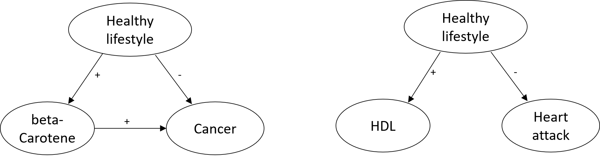
Of course, this issue has been known for almost a century, and the ideal solution for teasing out possible causation from correlation is to perform a randomized trial. An influence diagram (in plate notation) for a generic randomized trial that measures the causal effect of on is shown in Figure 20. Here, a coin is flipped for each of subjects. Depending on the outcome of the flip, an intervention is performed that forces to be one of two values, and is then observed. The randomized trial accurately assesses the causal effect of on , because the coin flip breaks the causal influence of the confounders on . In effect, the coin flip is a force/set/do decision without the alternative of “do nothing.” Unfortunately, the randomized trial is often an unattainable ideal. Such trials can be extremely expensive. Sometimes, ethical considerations preclude a randomized trial (e.g., when attempting to determine the effects of smoking on cancer). Also, study subjects often fail to comply with the intervention.

All attempts to solve this problem involve making assumptions. Basically, the goal is for the analyst to construct an argument that people will accept. The more reasonable the assumptions, the greater the number of individuals who will accept the argument.
One solution is to replace the coin flip with a natural intervention. As shown in Figure 21, this variable is called an instrumental variable. In order for the instrumental variable to accurately uncover the causal effect of on , it must obey the independence assumptions shown in the figure. In particular, the instrumental variable must be independent of the confounder(s), and the instrumental variable must be independent of , given and the confounder(s). In addition, the instrumental variable must have a direct effect on . One interesting point here is that, if there is no causal effect, and if the instrumental variable and are independent, then the two independence assumptions are satisfied. So, in this case, the assumptions don’t need to be left to debate—they can be demonstrated with data.

Voight et al. [79] used genetic markers as instrumental variables to investigate the effects of HDL increasing drugs on the incidence of heart attack. (In general, when the instrumental variable is a genetic marker, this process is called Mendelian randomization.) He found genetic markers that had a direct effect on HDL but were independent of incidence, and thus concluded that raising HDL had no effect on incidence. If only this work had been done before the drug companies spent billions on drugs development.
Another common approach for dealing with confounders is to use observational data only, avoiding interventions, and assume that a complete set of relevant confounders are observed. ([75] second edition, p.209, and [64] second edition, p.79, provide an algorithm for identifying such a set.) In this approach, the causal effect of and is estimated by weighting each observation with one over the probability of given the confounder(s). This approach, known as propensity score weighting, was first introduced by Robins and others in 2000 [68]. This approach has been typically applied to problems where is finite and has a relatively small number of values. Recently, however, Taha Bahadori, Eric Tchetgen, and I used deep learning to create an approach that can provide an accurate estimate when is continuous [5] [arXiv:2107.13068].
Another approach is to use DAG model learning that includes a deliberate search for confounders. Let’s consider an example taken from [36] [arXiv:2002.00269]. Sewell and Shah [71] measured the following variables for 10,318 Wisconsin high school seniors: Sex (): male, female; Socioeconomic Status (): low, lower middle, upper middle, high; Intelligence Quotient (): low, lower middle, upper middle, high; Parental Encouragement (): low, high; and College Plans (): yes, no. The data are described by the sufficient statistics in Table 1. Each entry denotes the number of cases in which the five variables take on some particular configuration. The first entry corresponds to the configuration SEXmale, SESlow, IQlow, PElow, and =yes. The remaining entries correspond to configurations obtained by cycling through the values of each variable such that the last variable (CP) varies most quickly. Thus, for example, the upper (lower) half of the table corresponds to male (female) students.
| 4 | 349 | 13 | 64 | 9 | 207 | 33 | 72 | 12 | 126 | 38 | 54 | 10 | 67 | 49 | 43 |
| 2 | 232 | 27 | 84 | 7 | 201 | 64 | 95 | 12 | 115 | 93 | 92 | 17 | 79 | 119 | 59 |
| 8 | 166 | 47 | 91 | 6 | 120 | 74 | 110 | 17 | 92 | 148 | 100 | 6 | 42 | 198 | 73 |
| 4 | 48 | 39 | 57 | 5 | 47 | 123 | 90 | 9 | 41 | 224 | 65 | 8 | 17 | 414 | 54 |
| 5 | 454 | 9 | 44 | 5 | 312 | 14 | 47 | 8 | 216 | 20 | 35 | 13 | 96 | 28 | 24 |
| 11 | 285 | 29 | 61 | 19 | 236 | 47 | 88 | 12 | 164 | 62 | 85 | 15 | 113 | 72 | 50 |
| 7 | 163 | 36 | 72 | 13 | 193 | 75 | 90 | 12 | 174 | 91 | 100 | 20 | 81 | 142 | 77 |
| 6 | 50 | 36 | 58 | 5 | 70 | 110 | 76 | 12 | 48 | 230 | 81 | 13 | 49 | 360 | 98 |
Reproduced by permission from the University of Chicago
Press.
©1968 by The University of Chicago. All rights
reserved.
As a first pass, I analyzed the data assuming there are no confounders. To generate priors for the model parameters, I used the method described in Section 4.2 with an equivalent sample size of 5 and a prior Bayesian network where the joint distribution is uniform. (The results were not sensitive to the choice of parameter priors. For example, none of the results reported here changed qualitatively for equivalent sample sizes ranging from 3 to 40.) I considered all possible structures except those where and/or had parents, and/or had children. The two graph structures with the highest marginal likelihoods are shown in Figure 22.

Some of the results are not surprising—for example the causal influence of socioeconomic status and IQ on college plans. Other results are more interesting. For example, from either graph we conclude that sex influences college plans only indirectly through parental influence. Also, the two graphs differ only by the orientation of the arc between PE and IQ. Either causal relationship is plausible.
The most suspicious result is the suggestion that socioeconomic status has a direct influence on IQ. To question this result, I considered additional graph structures with hidden variables. As the approach in Section 4 requires complete observations on all variables, I asked Radford Neal to apply his method known as annealed importance sampling, a Monte-Carlo technique [61], to compute the marginal likelihoods. Among the models considered, there were two with equal marginal likelihoods that were much higher than the marginal likelihoods of the best structures without hidden variables. They are shown in Figure 23. In the upper model, the confounder is a hidden common cause of and (e.g., parent “quality.”). In the lower model, is a cause of as in the best model with no hidden variables, and helps to capture the orderings of the values in the discretized versions of and . This example illustrates that learning DAG models can leave us uncertain. Assuming these two models are equally likely a priori, they remain equally likely given the data. A consolation is that we can average over the graph structures to make decisions or generate probabilities over various causal claims.
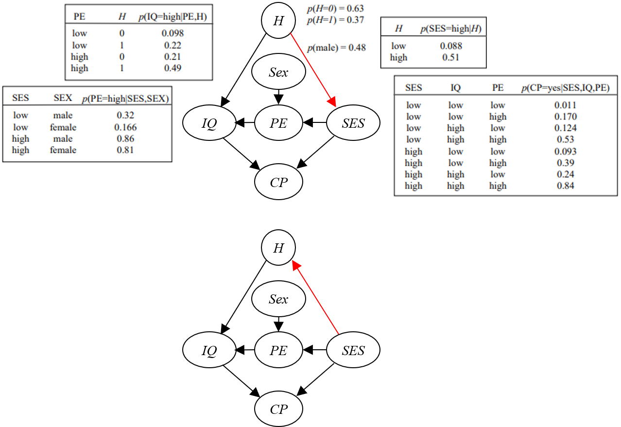
Finally, when learning fully causal DAG models, we can get lucky. For example, consider the graph structure for observed variables , , , and , shown in Figure 24. If there were one or more hidden confounders of to , there would be additional dependencies among the observed variables. Consequently, the structure shown in the figure would have a lower posterior probability than some other structure over the observed variables. As a result, if the structure shown in the figure has a high enough posterior probability, then we can conclude that the arc from to is not confounded. A similar argument applies to a graph structure as in the figure, but without the arc from to .

The bottom line is that, when an ideal randomized trial is not available, assumptions are needed to argue for a causal relationship. The good news is that the stigma in academics of talking about causality has largely gone away, and many researchers are now working to devise methods with assumptions that are more and more reasonable in practice.
4.6 Deep Learning
At this point in reading through the manuscript, you are almost certainly wondering: what about deep learning? Over the last decade, deep learning has made great advances in machine learning. Almost everyone in the world has been touched by its accomplishments. Yet, with just one exception, I have so far focused only on traditional ML. So here, I touch on several fundamental points about deep learning.
The first point is that a deep learning model is a graphical model (often a DAG model), but with several differences in emphasis from a traditional DAG model. One difference is that a deep model often represents a function from inputs to outputs rather than a joint distribution over all variables. A related difference is that a deep model is typically arranged in layers of nodes where only the input and output layers correspond to definitive observations in the real world. As one moves from the input layer to the output layer, each subsequent layer consists of unobserved variables that represent an incremental transformation from the previous layer. For example, in a convolutional deep model, the input layer consists of pixels on a screen, and subsequent layers correspond roughly to edges and lines, and then shapes, and then objects in the image. Interestingly, the visual cortices of primates have a similar organization [4].
The abundance of hidden variables in deep models leads to another set of differences. One is that a deep model can represent very complex functions. Another is that a deep model requires a large amount of data for training before its performance exceeds that of a traditional model. These two differences are illustrated by the curves shown in Figure 25. These curves, known as learning curves, plot algorithm performance as a function of the amount of data available to train the algorithm. Traditional ML is superior when there are small amounts of data, whereas deep learning is superior there are large amounts of data. The reason underlying the difference is simple: traditional methods encode prior knowledge either explicitly (i.e., they are Bayesian) or implicitly, and this prior knowledge gives those methods the edge when small amounts of data are available for training. The downside of relying on prior knowledge is that it is not perfect and, as the data available for training grows, these imperfections constrain the ability of the traditional methods to excel. The large number of hidden variables in a deep model also makes the explanation of its predictions more difficult.

A third point is that, if you accept the von Neumann–Morgenstern properties, you are bound to the prescriptions of decision theory for making decisions. This adherence holds whether you use traditional ML or deep learning. Of course, for low stakes decisions, it may be fine to append some ad hoc decision making to the output of deep learning—for example, a system that makes product recommendations could recommend products with the highest-value outputs. For high stakes decisions, however, following the MEU principle, which requires probability distributions over uncertainties, is a must. This point is important because a deep model often lacks a probabilistic component. Fortunately, it is always possible to augment a deep model to output probabilities for decision making. For example, when a deep learner outputs a number for a binary target variable, calibration procedures exist to map the output to a probability. For a discussion of calibration and its relationship to proper scoring rules, see [30].
A related final point is that a deep model (actually, any single-output neural network) can be used to represent the conditional probability distribution associated with a parent–child relationship in a traditional DAG model. I mentioned this point in [36] [arXiv:2002.00269], and such use is becoming more and more widespread [76] [ICLR 2021].
5 Applications: Fun with uncertainty, decision making, and graphical models at Microsoft Research
This section is all about some of the applications I was lucky enough to build while at Microsoft Research (MSR). I present them roughly in the order in which they were conceived and don’t rehash the technical details—you can read the original publications if you are interested. Mostly, I tell stories about how they came to pass. As you’ll see, my early work centered around expert systems and then evolved into machine learning. Nathan Myhrvold hired me to work on expert systems, but when I got to MSR, I quickly realized we had too few experts but lots of data. So, I began to teach myself machine learning, which—no surprise—eventually led to all sorts of high-impact applications. I am so grateful to Bill Gates, Nathan Myhrvold, and Rick Rashid for starting MSR and for letting those of us who were lucky enough to be there to explore whatever paths we thought were promising.
The first application I initiated was the Answer Wizard, an expert system that takes short text queries such as “How do I print sideways?” and provides an answer. The project came about during my first few days at Microsoft when I started to use Excel for the first time and couldn’t figure out how to make a graph. I tried the help function, but it didn’t know what a graph was. When I found someone at MSR to help me, they said, “Oh, you want to make a chart.” I thought to myself, “Who calls these things ‘charts’? Did the person who wrote the user interface like sailing?” It immediately occurred to me that I could build a diagnostic Bayesian network, much like Pathfinder, that related possible tasks the user wanted to perform to words or phrases they might use to describe those possible tasks. Just days later, Erich Finklestein and Sam Hobson, who were working on what would become Office 95 met with me. (To this day, I don’t know how they found me. My guess is that Nathan was funneling people in product groups to me.) They too were thinking about how the user could more easily discover functionality within Office. The Answer Wizard was born. You can find the technical details in [41] [arXiv:1301.7382].
The Answer Wizard still exists today. It’s a type-in box at the top of Office applications that says, “Tell me what you want to do,” which closely resembles its original form in Office 95. That said, for several years starting in the late 1990s, it got a lot of attention when an animated paper clip, named “Clippy,” served as its front end (see Figure 26). When the designers of Clippy first showed it to me, they said they would have about five different characters from which the user could select, Clippy being one of them. I asked, “Could you make one of the characters the invisible man [a famous comic-book character]?” My intent was to suggest that they leave the user interface alone. They understood my intent and were not pleased with my suggestion. In some sense, however, I think I got it right, at least at the time, as the character quickly became perceived as too silly and too annoying. That said, the character worked its way into the hearts of many, even becoming a popular Halloween costume. I hear rumors that Microsoft may bring it back. With hindsight, they should be able to make it less annoying. And with modern-day machine learning, they should be able to make it more useful.

The next project, the Windows Troubleshooters, began just weeks after the Answer Wizard. Phil Fawcett, working on the Product Support team, sought me out. (Again, I’m guessing this came from Nathan’s direction.) Phil was looking for ways that product support could be automated. As an example, he mentioned that many Windows customers were having problems with printing. To me, the problem seemed similar to the task of medical diagnosis, so I set out to solve the problem in a similar way. Soon, however, I learned an important difference: unlike medical diagnosis, where clues about the diagnosis come in the form of pure observations, device troubleshooting requires clues that come from a mix of interventions and observations. For example, when troubleshooting a print problem, one could observe a symptom, then turn the printer off and then on again, and re-observe to see if and how that symptom had changed. Having had lots of experience with influence diagrams and causal reasoning by this time, it was straightforward to adapt the technology I had built for medical diagnosis to this new task. You can find the details at [9] [arXiv:1302.3563]. As I was coding the troubleshooting algorithms, Jack Breese arrived as the second member of our group at MSR. We called it DTG—the Decision Theory Group. He developed an elegant user interface for the troubleshooters, and together we refined the fully causal model for print toubleshooting (see Figure 27). We demoed the system to Phil Fawcett, and the Windows Troubleshooters were born. They were popular for at least a decade, but eventually got replaced when sufficient problem–solution pairs were collected and could be searched.

The next project was one of my first forays into a machine-learning application. It was 1994. I had just formed the Machine Learning and Applied Statistics group at MSR and was armed with the theoretical work on learning DAG models from data. I attended a workshop on this new idea called collaborative filtering. The idea was explained more as an algorithm than a task. In particular, it was explained as recommending items (e.g., movies, websites) to a user that they might like, by identifying other users who liked similar items, and then recommending items that the others liked that the original user did not know about. Right there during the workshop, I realized that the task was a prediction problem: given data on liked items by a set of users, predict other items that each person would also like. Furthermore, I thought that, while similarity-based methods would be one way to address the task, it would be worth trying other prediction algorithms to see if they worked better.
Over the next few months, Carl Kadie (new to the DTG team) and Jack Breese, began exploring various algorithms on multiple datasets. As an example, let’s consider one of my favorites: Nielsen rating data for TV shows. For every user and every TV show, Nielsen recorded whether the user watched the show during February sweeps week in 1995. For every show, we built an (ML) decision tree with that show as the classification variable, using all other TV shows as prediction variables. The results made a lot of sense. If you watched Seinfeld, you were likely to watch Friends. And if you watched Seinfeld and didn’t watch Friends, it was worth recommending Friends to you. Another good example was that, if you liked watching Matlock, you would likely enjoy 60 Minutes. For more details, see [10] [arXiv:1301.7363].
The approach was a big hit at Microsoft and in the business world in general. It became so popular that the technology shipped in Microsoft Commerce Server 2000. It also caught the eye of Bill Gates, who asked me to present the work at a large conference with him. The presentation consisted of showing a visualization of the model applied to the Nielsen data, which I had set up on my laptop, and I remember being quite nervous before the presentation. “I had better not screw this up,” I thought to myself. It turns out that I was so nervous that I had forgotten to plug the charger into my laptop. Immediately after finishing the presentation, I looked at my laptop and it went dark. I had barely avoided a major disaster.
The work on collaborative filtering led to the creation of a new type of graphical model, which I unimaginatively called the dependency network. In this approach, rather than construct a directed acyclic model, one constructs a typically cyclic graph, where each child variable has all other variables as possible parents. The missing arcs reflect conditional independence—in particular, , but now many or all of the arcs in the dependency network are bi-directional. A dependency network structure for the Nielsen data is shown in Figure 28.
When predicting a target variable from observations of all other variables, we can just look up the result from that target’s local distribution. If more complex inference is needed, we can use Gibbs sampling. In this approach, we begin by assigning random values to every variable. Then, we cycle through each variable, sampling a new value for it, based on the values of its parents’ variables. We keep track of the distribution on these samples, which in the limit yields a joint distribution over the variables.

This model and inference approach leads to several interesting mathematical results. To understand these results, first note that the local distributions may be consistent or inconsistent with one another. Inconsistency is likely when the local distributions are learned independently. For example, consider the simple domain consisting of two variables and . Is it possible that an estimator of discards as an input, whereas the estimator of retains as an input. The result is the structural inconsistency that helps to predict , but does not help to predict . Numeric inconsistencies are also likely. Nonetheless, in situations where the data set contains many samples, strong inconsistencies will be rare because each local distribution is learned from the same data set, which presumably is generated from a single underlying joint distribution. In other words, although dependency networks will be inconsistent, they will be “almost” consistent when learned from data sets with large sample sizes.
So first, let’s consider consistent dependency networks. In this case, every arc in the graph structure must be bi-directional, so we may as well replace these bi-directional arcs with undirected edges, yielding an undirected graph structure. Given this observation, a question arises as to whether the dependence network is equivalent to another undirected network known as a Markov random field (also known as a Markov network) as originated by Julian Besag. Instead of Gibbs sampling, Julian’s approach performs inference using distributions on subsets of variables corresponding to cliques in the undirected graph structure. In 2000, Max Chickering, Chris Meek, and I showed that, indeed, a consistent dependency network for a domain of finite variables is equivalent to a Markov random field, provided all local distributions are positive [38] [jmlr/v1]. Here, by “equivalent”, I mean that, given an undirected graph structure, any distribution represented by one approach can also be represented by the other. It is interesting to note that Julian started with directed dependency networks, but instead of taking the path of Gibbs sampling for inference, took the path involving distributions on cliques. When I showed this work to Julian, he said, “I wish I had thought to use Gibbs sampling back then—it would have been so much simpler.”
What happens with consistent dependency networks when we relax the assumption that distributions are positive? In the case of undirected networks, different definitions, while equivalent when distributions are positive, are no longer equivalent [56]. Thomas Richardson, Chris, and I characterized the distributions representable by dependency networks in the non-positive case, and showed that there are distributions representable by dependency networks that are not representable by various definitions of undirected network, and vice versa [42] [10.14736/kyb-2014-3-0363].
What happens when dependency networks are inconsistent? In the same publication [38] [jmlr/v1], Max, Chris, and I showed that Gibbs sampling will still converge to a unique distribution, provided the local distributions are positive. This distribution may not be consistent with the local distributions and can depend on the order in which the Gibbs sampler visits each variable, but convergence is nonetheless guaranteed.
This next application is a bit out of time order, as I’m saving the best for last. In early 2000, Microsoft services were in full bloom. Steven White from msnbc.com contacted me, hoping to gain a better understanding of how customers were using their new site. Having recently completed work on unsupervised learning with mixture models (e.g., [16] [10.1023/A:1007469629108], [77] [arXiv:1301.7415]), I suggested that we try clustering customers’ behavior. Steven was particularly interested in the sequence of pages visited on the site, so I came up with the idea of learning and then visualizing a mixture of time-series models. I suggested we start with a very simple version—a mixture of first-order Markov models. This simple approach turned out to be quite useful. Together, Igor Cadez, who joined my team as summer intern, Padhraic Smyth, Igor’s PhD advisor, and Chris Meek built WebCanvas [13] [10.1145/347090.347151]. We took page visits from about one million user sessions on msnbc.com, learned the model, used the model to assign each user session to a cluster (i.e., a mixture component), and then displayed representative samples from each mixture component. The result is shown in Figure 29.

Steven used the model on the msnbc.com data and derived a number of unexpected, actionable insights. For example, there were a large number of hits to the weather pages (cluster 1), there were large groups of people entering msnbc.com on tech (clusters 11 and 13) and local (cluster 22) pages, there was a large group of people navigating from on-air to local (cluster 12), and there was little navigation between tech and business sections. I mention this project because, to this day, I regularly get requests for the code. It seems to remain a useful tool.
Perhaps the most impactful non-medical project that I initiated at Microsoft was, to my knowledge, the world’s first ML-based spam filter. It was late 1996, and I started to get a new type of email. This email was coming from people I didn’t know and was usually asking me to buy something. In early 1997, as shown in Figure 30, I got a “burst” of emails—three in less than 24 hours! This was the straw that broke the camel’s back. Even though I had only received about a dozen of this new type of message, I knew it was going to become a big problem. Sixteen minutes after seeing the third message, I sent an email to Eric and Jack: Figure 31.


I followed up with an email asking Eric and Jack to start saving their email, so we could use it for training. Within a few months, Mehran Sahami spent an internship at MSR and built our first machine-learning spam filter. We tried several classifier methods, including Bayes nets and (ML) decision trees, but the approach that worked best was suggested and implemented by John Platt: the Support Vector Machine. Because we wanted the classifier to output probabilities for decision making (do we label the email as spam or not?), John was motivated to calibrate the classifier output and invented Platt Scaling.
Our spam filter was a big hit and, in 1998, it almost shipped in Outlook Express, a free and (ironically) feature-light version of Outlook. While still in beta release, however, Microsoft got a call from Blue Mountain, a greeting card company, complaining that the spam filter was blocking its greeting cards when a user-controlled threshold knob in the filter was set to a low setting. We immediately met with them, appreciated the problem, and said we would have it fixed by the end of the week. Before the end of the week came, however, Blue Mountain sued Microsoft for deliberately trying to ruin their business. Despite our reassurances and despite the fact that Outlook Express was still in beta, Blue Mountain supported their claim by pointing to a single email greeting card that Microsoft had made available to its customers that, at the filter threshold blocking Blue Mountain, made it through our filter.
The media went wild. Readers accepted Blue Mountain’s claim without hesitation. Microsoft was “obviously guilty.” Here’s just one blog from boards.fool.com:
Why would Microsoft want to prevent electronic greeting cards from being delivered? It turns out that after an unsuccessful attempt to purchase Blue Mountain Arts, Microsoft started its own electronic greeting card service. The “bug” in Outlook Express appeared at about the same time that Microsoft’s greeting card service began.
I got my first, brutal taste of “fake news.” The spam filter was promptly removed from Outlook Express.
Years went by. Spam got more voluminous and annoying, but Microsoft refused to ship a spam filter. Finally, Bryan Starbuck, a programmer in MSN 8 did something about it. He stumbled on our code and knew that shipping it was the right thing to do. His plan was to sneak it into the release and wait until just before release to tell others about it, when it would be at high risk to remove. His plan worked. The spam filter shipped in MSN 8 in 2002. This time, it was well received. Just a few months after release, the spam filter was the focus of Microsoft’s Super Bowl commercial. A snapshot is shown in Figure 32. Once the ice was broken, it became a no-brainer to ship it in other Microsoft products including Outlook and Exchange Server.

Besides the Blue Mountain suit, there is one other regret I have about the path that our spam filter took. In our original versions, the filter was personalized to the user’s email. The user would (optionally) populate a junk-mail folder, and an ML classifier would run in the background, constantly updating the filter. It worked really well. For hundreds of correct calls, there was typically only one false positive. For some reason, however, senior leadership decided that asking the user to maintain a junk-mail folder was too onerous and instead asked users to identify good senders versus junk-mail senders. To this day, I spend at least an hour a month going through my junk mail, because my one-size-fits-all filter has so many false positives.
An immediate spinoff of the spam-filter work was text categorization, which first shipped in Microsoft Sharepoint Portal Server 2001. Here, personalization was central. A user would create a category folder, drop documents into it, and the system would suggest likely categories for new documents. For technical details on spam filtering and text categorization, see [69] [AAAI:WS98-05-009] and [22] [10.1145/288627.288651], respectively.
6 Applications in healthcare
I’ve already highlighted some of the healthcare applications I worked on while at Stanford. When I first got to MSR, despite my interest in continuing this work, Nathan asked me to focus on non-healthcare applications. Nonetheless, in my first few years there, MSR began to grow exponentially. Soon, Nathan and Rick opened things up, saying that we could work on just about anything we wanted to. So, I began re-exploring healthcare applications.
The first application was a no-brainer. In 1994, Steven Freedman, who went to Medical School with Eric and me at Stanford, joined Microsoft to build one of Microsoft’s first internet experiences, a system to help young families manage pregnancies and the health issues of their children. Steven, knowing about Pathfinder, Intellipath, and Knowledge Industries, asked Eric and me to contribute to this system by constructing an expert system to address diagnostic challenges in this space. The work was straightforward, but rewarding. Microsoft Pregnancy and Child Care was born.

Figure 33 shows a screenshot at the beginning of a diagnostic case. A parent has just told the system that her young toddler has a sore throat. The system infers a probability distribution, shown on the right, and is about to ask questions of the parent to narrow the list of possible diagnoses. The project was a technical success, but never saw release. An important customer of Microsoft asked Steve Ballmer to kill the project, because they were working in the same space. Steve complied and, sadly to this day, no similar project has been released by that customer. Another somber note: In those days, Microsoft had lavish parties to celebrate the new release of a product. The cancellation of the project came just days before the release party, so the party went on as scheduled with the more than the 100 people who worked on the project. It was a very depressing party.
Another large project was my work to create a vaccine for HIV. It was 2004, and I had just formed the Bioinformatics group at MSR. Nebojsa Jojic and I visited Jim Mullins, a prominent HIV scientist at the University of Washington. Both Nebojsa and I immediately got excited about the prospect of using machine learning to advance what was already a massive effort to construct a vaccine for HIV. The excitement was mutual. Jim introduced us to Rick Klausner, who introduced us to Simon Mallal, who introduced us to Bruce Walker, who introduced us to Nicole Frahm, Zabrina Brumme, Florencia Pereyra, and Marry Carrington, among others. At Microsoft, several folks including Carl Kadie and Jonathan Carlson joined the effort. We made good progress on the goal. Here, I won’t go through the dozens of manuscripts that resulted, but I will summarize one line of work, which remains promising.
There is an interesting analogy between spam filtering and HIV vaccine design that helps to explain this work. When our first spam filter came out, spammers figured out clever ways to work around it. For example, spammers would encode sensitive words like “Viagra” in bit maps, so our filters wouldn’t recognize the occurrence of the word. In response, we would change our filters to catch this case, but the spammers would just adapt again. The battle was on. Eventually, we realized that we had to try to find an Achilles heel of the spammers—something they couldn’t adapt away from. We found one: spammers needed to make money. At the time I worked on this problem, there were only a relatively small number of sites that could process payments. We catalogued those sites and used any reference to such a site as a key feature for predicting whether a message was spam. The approach worked well.
Remarkably, we experienced something similar when working on HIV. Our immune system attacks HIV by killing cells that harbor the virus. In response, the virus mutates to avoid the attack. More specifically, just about every cell displays peptides, short fragments of proteins manufactured inside the cell, on its surface. The peptides are displayed on HLA molecules, proteins coded for by three HLA genes on chromosome six. Each of these three genes have hundreds of varieties and, consequently, individuals rarely attack all the same HIV peptides. This diversity is a good thing. If there wasn’t such diversity, then a virus (HIV or otherwise) that killed one of us would kill all of us. (Each of us has one or two varieties of each of the three genes—one from mom and one from dad. It’s better when a person has two different versions of each gene to maximize the variety of viruses that can be attached. Interestingly, there is scientific evidence that a women can literally smell the HLA molecules of a man and is attracted to men that have different varieties then she does. Perhaps the chemistry of love is indeed chemistry.) Constantly, T-cells come into contact with the cell to check that these peptides are not foreign to the body. If they are, the T-cell gets excited, which leads to the creation of T-cells that can kill any cell presenting one or more foreign peptides. Unfortunately, when this killing happens, HIV mutates to avoid attack. It turns out that HIV is a very robust virus that can thrive with many mutations. A single individual will typically harbor thousands of different HIV varieties. Herein lies the analogy. The immune system is like the spam filter, and HIV’s ability to mutate and thrive is like a spam email’s ability to exist in many forms and still get the message across (such as including “Viagra” in a bit map).
To continue the analogy, a key question becomes: does HIV have an Achilles heel? Evidence that it does comes from the observation that there is a small fraction of humans, called “controllers,”, who naturally control HIV—that is, they get infected with HIV, but don’t go on to develop serious disease. One causal hypothesis is that these controllers have HLA molecules that attack the virus in vulnerable positions along HIV proteins. To test this hypothesis Bruce Walker and team identified the HLA molecules, targeted peptides, and the presence or absence of control in 341 individuals infected with HIV. My team determined the likelihood of data from the causal model in Figure 34a and compared it to the likelihood of a causal model for an alternative hypothesis shown in Figure 34b. The alternative hypothesis is that HLA directly causes control, and that the lack of control leads to a proliferation of HIV varieties that determines which peptides are targeted. The first hypothesis had a significantly higher likelihood [66] [10.1128/JVI.01004-14].

Learning graphical models also help identify which parts of the virus are attacked by our immune system, a key task in HIV vaccine design. There are many locations or positions to attack. The HIV genome is over 9,000 nucleotides long and codes for the production of nine primary proteins with over 3,000 amino acids. Each amino acid position is a possible target for attack. As just discussed, the task of identifying targets is complicated because there is a lot of variation in the human immune system from person to person, and each variation can attack different parts of HIV. So, the task of identifying attack targets amounts to identifying correlations between a person’s particular HLA molecules and the particular amino acids at each position along HIV’s sequence. A difficulty with this approach is that HIV sequences are constantly evolving as they pass from one individual to the next, and so history is a confounder of the correlations. An example is shown in Figure 35.

In the figure, there are two different evolution histories—sometimes called phylogenies—that result in observations of amino-acid or at a given HIV sequence position. The shaded nodes are observed; the unshaded nodes are not. Also shown are whether the individuals with observed HIV sequences have a particular HLA variety or not. In both possible histories, there are four individuals with a particular HLA and an observed amino-acid , and four individuals with the lack of that HLA and amino-acid at the same position. When analyzed naively, the correlation between the presence or absence of the HLA and the presence of versus at this position is substantial. Now, however, consider the two histories. In the first history, the amino-acid is transmitted from person 1 to person 2, but person 3 gets a mutated . In the second history, all three persons have amino-acid —all mutations to happen in the persons observed. In the first history, the evolution from person 1 to persons 2 and 3 explain the correlation. In the second history, the presence or absence of the particular HLA explains the evolution. That is, the second history is much stronger evidence that the particular HLA molecule is causing the mutation.
To take phylogeny into account when identifying HLA–amino-acid associations, Jonathan Carlson, Carl Kadie, and I developed a system called PhyloD [14] [10.1371/journal.pcbi.1000225]. At the core of the system is a DAG model, a simple example of which is shown in Figure 36. Again, shaded nodes are observed; unshaded nodes are not. The structure of the phylogeny is learned from the amino acids observed at all sequences. Given observations of the shaded nodes, the system uses the Expectation–Maximization algorithm to infer distributions on the unobserved variables. To determine the strength of the association between and , the likelihood of the data for this model is compared to a null model with only the observations. Of course, a Bayesian approach could be used, but this frequentist approach was computationally efficient and effective.

Before 2012, my work on HIV was getting modest attention by senior leadership at Microsoft. Then, something random happened that changed that. My son’s elementary school asked me to speak to their graduating class. I was happy to do it, but it took me a week or so to create a talk for the class that was simple enough for them to understand. The kids loved it, so I decided to give it a try at Microsoft. Leadership loved it and asked me to speak at the 2013 Microsoft Worldwide Partner Conference with many thousands of people in attendance. You can see the talk on [youtube]. There’s lesson in here somewhere.
The work on PhyloD led to a useful genomics tool. In 2001, the first human genomes were (almost completely) sequenced by teams led by Craig Venter and Francis Collins for 300 million dollars and 3 billion dollars, respectively. Today, sequencing the human genome costs about 500 dollars. This is quite impressive, given that the human genome consists of about three billion nucleotide pairs. As a result of this accomplishment, there has been a flood of genomics data leading to important findings and applications.
One important finding is that, remarkably, the differences between two individuals’ DNA are extremely small—about 0.1%. That is, if you look at the three billion As, Cs, Ts, and Gs in the human genome (times two, because we each have two copies of DNA, one from mom and one from dad), you’ll only find millions of differences—called single nucleotide polymorphisms or SNPs. (There are also more complex differences such as insertions, deletions, and multiple copies of small regions of DNA, but I won’t get into that here.) These “small” differences are a big plus for computer scientists and computational biologists who are working with and analyzing genomic data, as it drastically reduces the scale of their computational problems. Another interesting finding is that almost all SNPs take on only two of the four possible nucleotide values (A, T, C or G), which makes it possible to talk about each SNP as a binary variable with a major and minor nucleotide or allele.
Perhaps the most compelling application of the genomics revolution is personalized or precision medicine, where medical care is customized to the patient based on their genome. As an example, it turns out that if you happen to have a particular set of SNPs in the region of your DNA that codes for the HLA molecules, then if you take carbamazepine (a drug that suppresses seizures), you will very likely develop Stevens-Johnson syndrome, a horrible disease where layers of your skin separate from one another [23]. One idea behind personalized medicine is to avoid such fates by checking your genome before administering drugs. More generally, with personalized medicine, your genome could be used to identify drugs that would work well for you or to warn you of diseases for which you are at high risk, such as diabetes and heart disease, so you can take measures to avoid them.
This application brings us to the question: How do we identify associations between your genome and various traits such as whether you will get a disease or whether a particular drug will harm you? Although older techniques have been used for decades, the genomics revolution has led to the use of a new technique known as Genome-Wide Association Studies or GWAS. With GWAS, you identify a set of individuals, measure many or all of their SNPs, and then identify correlations between those SNPs and one or more traits.
One surprising realization from these studies is that the Stevens-Johnson-syndrome example—where only a few SNPs are associated with the trait—is the exception rather than the rule. Namely, it is now recognized that, typically, many SNPs (hundreds and more) are causally related to a single trait [2]. Furthermore, it turns out that whether an association can be detected depends on the frequency of the minor allele and the strength of the SNP’s effect on the trait. SNPs with larger effect tend to have very rare minor alleles due to natural selection. In contrast, SNPs with more common minor alleles tend to have little effect on the trait. Thus, extremely large sample sizes—hundreds of thousands or more—are required to create a comprehensive picture of the relationships among SNPs and traits. Many groups including the governments of the US and England are working to generate such data. Unfortunately, large data sets often lead to the introduction of confounders. As an example, a data set might include individuals with different ethnicities. In this situation, if one ethnicity is correlated with both the trait and a SNP, then the trait and a non-causal SNP will be correlated. Confounders of this sort are known as population structure. In large data sets, we also often see individuals who are related to each other, either closely or distantly. These relationships, known as family relatedness, also introduce correlations among SNPs and traits that are not causally related.
This issue raises the question: How can we deal with confounders and identify only the truly causal associations? When I first heard about this problem from an intern, Noah Zaitlen, I immediately thought of adapting PhyloD to solve the problem. I replaced amino-acid identity with trait and HLA with SNP. It was also clear that a phylogeny would not adequately reflect the evolutionary history of humans, as we have two copies of each piece of DNA, whereas HIV has only one copy. So, I replaced the phylogeny with a continuous hidden variable for each individual and modeled these variables jointly with a multivariate-Gaussian distribution whose covariance matrix represents the similarity among individuals and is learned from the available SNPs for each individual. An example graphical model for four individuals is shown in Figure 37.

I discussed this model with Elezar Eskin, Noah’s advisor. In turn, Elezar discussed the model with Nicholas Schork, who recognized that it was equivalent to a linear mixed model (LMM), which had been used by animal breeders for decades. Elezar and team and I went on to publish the model, speeding up previous methods for estimating its parameters and demonstrating its use on several genomics datasets [52] [10.1534/genetics.107.080101]. Given a dataset with individuals and SNPs to be tested for association, the algorithm ran with computational complexity , which unfortunately was still too slow for most modern datasets. (Animal breeders typically analyzed datasets with dozens or hundreds of samples.)
A real advance happened when Christoph Lippert joined our Bioinformatics group at MSR. Christoph identified algebraic manipulations that yielded exact results, but with computational complexity , where is the number SNPs used to infer the covariance matrix of the multivariate Gaussian [58] [doi:10.1038/nmeth.1681]. The algorithm, called FaST-LMM, is still in frequent use today.
Our group at MSR went on to develop many extensions to this work. For example, recognizing that we could further speed up the algorithm by reducing , we developed two ideas for doing so. One worked well and one worked horribly. The one that worked horribly was to estimate the covariance matrix with SNPs that were detectably correlated with the trait. We called this approach FaST-LMM-Select. The problem with the approach was that there was so much noise in the correlations between SNPs and trait, that we ended up throwing out the baby with the bathwater. Unfortunately, there was an error in one of the experiments that suggested the approach was working well (see Figure S1 from the original paper [60]), and we didn’t catch this error until several additional papers were published. The bottom line: don’t use FaST-LMM-Select.
The approach that did work well was to take advantage of linkage disequilibrium, the observation that nearby SNPs are highly correlated. Given this correlation, sampling SNPs (e.g., using every fifth SNP in order along the chromosome) to estimate the covariance matrix yields results that are quite close to exact [81] [doi: 10.1038/srep06874].
Regarding linkage disequilibrium, when applying LMMs to real data, I noticed that statistical power was lost when SNPs near the SNP being tested (and the test SNP itself) are included in the estimation of the covariance matrix. This is not surprising: when including such SNPs in the estimation, the correlation matrix “steals” part of the impact of the test SNP on the trait, thus diminishing the estimate of that impact [58] [doi:10.1038/nmeth.1681]. (The same principle applies to PhyloD.) This observation led to what is now a standard of practice in GWAS known as “leave out one chromosome.” That is, when testing a SNP on a particular chromosome, use a covariance matrix estimated with SNPs from all but that chromosome.
Another extension of FaST-LMM involved testing for associations between a set of SNPs (e.g., those associated with a particular gene) and a trait. The approach essentially combines very weak signals, yielding increased statistical power [59] [10.1093/bioinformatics/btu504]. Other extensions sped up the identification of SNP–SNP interactions that are associated with a trait [57] [10.1038/srep01099], and addressed situations where the presence of rare traits are over-represented in the data [80] [10.1038/nmeth.3285]. We also created a version of FaST-LMM that incorporated more than one covariance matrix—for example, when there is confounding both from SNP similarities and from environmental effects due to differences in spatial location [40] [10.1073/pnas.1510497113]. In addition, we optimized FaST-LMM for the cloud [51] [10.1101/154682].
I close with two stories about my genomics work. In 2006, after a meeting between Microsoft and MIT in Boston, I had the fortune to fly back to Seattle with Craig Mundie, who led Microsoft’s advanced technology efforts. We got to talking about the huge potential for genomics in general, and GWAS in particular, to health and wellness. Out of that discussion came the idea to build a service that would sequence customers’ SNPs, ask them about important traits, identify genome-wide associations, and inform them of traits they should look out for. We anticipated 23andMe and Ancestry. Unfortunately, although Microsoft filed a patent on the idea, and I tried repeatedly to generate interest within Microsoft to build the service, we were beaten to the punch.
Perhaps the most impactful outcome of my work in genomics came in 2010, when Bryan Traynor and team and I performed a GWAS on a cohort of Finnish individuals, some of whom had Amyotrophic Lateral Sclerosis (ALS). We found a signal on chromosome 9. Bryan then did the difficult work to find the precise mutation on the genome that was producing the signal: an expansion of the C9ORF72 gene consisting of a repeated six-nucleotide-long sequence [67] [10.1016/S1474-4422(10)70184-8]. Later, it was found that this mutation accounts for about 30% of inherited cases of ALS, and treatments based on this finding are now in clinical trials [54].
Acknowledgments
I sincerely thank Carl Kadie, Chris Meek, Dan Geiger, Eric Horvitz, Jack Breese, Jonathan Heckerman, Max Chickering, Ross Shachter, and Pedro Domingos for their comments on earlier drafts.
References
- [1] J. Aczel. Lectures on Functional Equations and Their Applications. Academic Press, New York, 1966.
- [2] H.L. Allen, K. Stefansson, T.M. Frayling, and J.N. Hirschhorn. Hundreds of variants clustered in genomic loci and biological pathways affect human height. Nature, 467:832–838, 2010. Other authors omitted for lack of space.
- [3] K. J. Arrow. A difficulty in the concept of social welfare. Journal of Political Economy, 58:328–346, 1950.
- [4] Robert Aung. Do convolutional neural networks mimic the human visual system?, 2021.
- [5] T. Bahadori, E.T. Tchetgen, and D. Heckerman. End-to-end balancing for causal continuous treatment-effect estimation. In Proceedings of the Thirty-ninth International Conference on Machine Learning, 2022.
- [6] T. Bayes. An essay towards solving a problem in the doctrine of chances. Biometrika, 46:293–298, 1958. Reprint of original work of 1763.
- [7] J.M. Bernardo. Expected information as expected utility. Annals of Statistics, 7:686–690, 1979.
- [8] J.M. Bernardo and A.F.M. Smith. Bayesian Theory. Willey, New York, 1994.
- [9] J. Breese and D. Heckerman. Decision-theoretic troubleshooting: A framework for repair and experiment. In Proceedings of Twelfth Conference on Uncertainty in Artificial Intelligence, Portland, OR, pages 124–132. Morgan Kaufmann, August 1996.
- [10] J. S. Breese, D. Heckerman, and C. Kadie. Empirical analysis of predictive algorithms for collaborative filtering. In Proceedings of Fourteenth Conference on Uncertainty in Artificial Intelligence, Madison, Wisconsin. Morgan Kaufmann, August 1998.
- [11] B.G. Buchanan and E.H. Shortliffe, editors. Rule-Based Expert Systems: The MYCIN Experiments of the Stanford Heuristic Programming Project. Addison–Wesley, Reading, MA, 1984.
- [12] W. Buntine. Operations for learning with graphical models. Journal of Artificial Intelligence Research, 2:159–225, 1994.
- [13] I. Cadez, D. Heckerman, C. Meek, P. Smyth, and S. White. Model-based clustering and visualization of navigation patterns on a web site. Data Mining and Knowledge Discovery, 7(4):399–424, 2003.
- [14] J. Carlson, Z. Brumme, C. Rousseau, C. Brumme, P. Matthews, C. Kadie, J. Mullins, B. Walker, P. Harrigan, P. Goulder, and D. Heckerman. Phylogenetic dependency networks: Inferring patterns of CTL escape and codon covariation in HIV-1 Gag. PLoS Computational Biology, 4, 2014.
- [15] K. Chaloner and G. Duncan. Assessment of a beta prior distribution: PM elicitation. The Statistician, 32:174–180, 1983.
- [16] D. Chickering and D. Heckerman. Efficient approximations for the marginal likelihood of Bayesian networks with hidden variables. Machine Learning, 29:181–212, 1997.
- [17] D. Chickering, D. Heckerman, and C. Meek. Large-sample learning of Bayesian networks is NP-hard. The Journal of Machine Learning Research, 5:1287–1330, 2004.
- [18] G. Cooper and E. Herskovits. A Bayesian method for constructing Bayesian belief networks from databases. In Proceedings of Seventh Conference on Uncertainty in Artificial Intelligence, Los Angeles, CA, pages 86–94. Morgan Kaufmann, July 1991.
- [19] R. Cox. Probability, frequency and reasonable expectation. American Journal of Physics, 14:1–13, 1946.
- [20] P. Dawid. Statistical theory. The prequential approach (with discussion). Journal of the Royal Statistical Society A, 147:178–292, 1984.
- [21] R. Duda, J. Gaschnig, and P. Hart. Model design in the PROSPECTOR consultant system for mineral exploration. In D. Michie, editor, Expert Systems in the Microelectronic Age, pages 153–167. Edinburg University Press, Edinburgh, Scotland, 1979.
- [22] S. Dumais, J. Platt, D. Heckerman, and M. Sahami. Inductive learning algorithms and representations for text categorization. In Proceedings of ACM-CIKM98. ACM-CIKM, November 1998.
- [23] H. L. Ferrell. Carbamazepine, HLA-B*1502 and risk of Stevens–Johnson syndrome and toxic epidermal necrolysis: US FDA recommendations. Pharmacogenomics, 9, 2009.
- [24] D. Geiger and D. Heckerman. Dependence and relevance: A probabilistic view. Technical Report 1611.02126, arXiv, 1993.
- [25] D. Geiger and D. Heckerman. A characterization of the dirichlet distribution through global and local independence. Annals of Statistics, 25:1344–1369, 1997.
- [26] D. Geiger and D. Heckerman. Parameter priors for directed acyclic graphical models and the characterization of several probability distributions. Annals of Statistics, 30:1412–1440, 2002.
- [27] W. Gilks, A. Thomas, and D. Spiegelhalter. A language and program for complex Bayesian modeling. The Statistician, 43:169–177, 1994.
- [28] N. Gisin. Quantum Chance: Nonlocality, Teleportation and Other Quantum Marvels. Springer, 2014.
- [29] C. Glymour. Markov properties and quantum experiments. In W. Demopoulos and I. Pitowsky, editors, Physical Theory and its Interpretation, volume 72, pages 117–126. Springer, 2006.
- [30] T. Gneiting, F. Balabdaoui, and A. Raftery. Probabilistic forecasts, calibration and sharpness. Journal of the Royal Statistical Society, B, 69:243–268, 2007.
- [31] I.J. Good. Good Thinking: The Foundations of Probability and Its Applications. University of Minnesota Press, Minneapolis, MN, 1983, 1983.
- [32] M. Hallett. Physiology of free will. Annals of Neurology, 80:5–12, 2016. Note the authors definition of free will.
- [33] D. Heckerman. Probabilistic interpretations for MYCIN’s certainty factors. In Proceedings of the Workshop on Uncertainty and Probability in Artificial Intelligence, Los Angeles, CA, pages 9–20. Association for Uncertainty in Artificial Intelligence, Mountain View, CA, August 1985.
- [34] D. Heckerman. An axiomatic framework for belief updates. In Proceedings of the Second Workshop on Uncertainty in Artificial Intelligence, Philadelphia, PA, pages 123–128. Association for Uncertainty in Artificial Intelligence, Mountain View, CA, August 1986.
- [35] D. Heckerman. A Bayesian approach for learning causal networks. In Proceedings of Eleventh Conference on Uncertainty in Artificial Intelligence, Montreal, QU, pages 285–295. Morgan Kaufmann, August 1995.
- [36] D. Heckerman. A tutorial on learning with Bayesian networks. In Learning in graphical models, pages 301–354. Kluwer, 1998.
- [37] D. Heckerman. Personal communication. 2014.
- [38] D. Heckerman, D.M. Chickering, C. Meek, R. Rounthwaite, and C. Kadie. Dependency networks for inference, collaborative filtering, and data visualization. Journal of Machine Learning Research, 1:49–75, 2000.
- [39] D. Heckerman, D. Geiger, and D. Chickering. Learning Bayesian networks: The combination of knowledge and statistical data. Machine Learning, 20:197–243, 1995.
- [40] D. Heckerman, D. Gurdasani, C. Kadie, C. Pomilla, T. Carstensen, H. Martin, K. Ekoru, R.N. Nsubuga, G. Ssenyomo A. Kamali, P. Kaleebu, C. Widmer, and M.S. Sandhu. Linear mixed model for heritability estimation that explicitly addresses environmental variation. PNAS, 113:7377–7382, 2016.
- [41] D. Heckerman and E. Horvitz. Inferring informational goals from free-text queries. In Proceedings of Fourteenth Conference on Uncertainty in Artificial Intelligence, Madison, Wisconsin. Morgan Kaufmann, August 1998.
- [42] D. Heckerman, C. Meek, and T. Richardson. Variations on undirected graphical models and their relationships. Kybernetika, 50:363–377, 2014.
- [43] D. Heckerman and R. Shachter. Decision-theoretic foundations for causal reasoning. Journal of Artificial Intelligence Research, 3:405–430, 1995.
- [44] D.E. Heckerman. Probabilistic Similarity Networks. MIT Press, Cambridge, MA, 1991.
- [45] E. Hewitt and L. Savage. Symmetric measures on cartesian products. Transactions of the American Mathematical Society, 80:470–501, 1955.
- [46] R.A. Howard. Risk preference. In R.A. Howard and J.E. Matheson, editors, Readings on the Principles and Applications of Decision Analysis, volume II, pages 629–663. Strategic Decisions Group, Menlo Park, CA, 1983.
- [47] R.A. Howard and J.E. Matheson, editors. The Principles and Applications of Decision Analysis. Strategic Decisions Group, Menlo Park, CA, 1983.
- [48] R.A. Howard and J.E. Matheson. Influence diagrams (1981). In R.A. Howard and J.E. Matheson, editors, Readings on the Principles and Applications of Decision Analysis, volume II, pages 721–762. Strategic Decisions Group, Menlo Park, CA, 1984.
- [49] J. J. Pratt and R. Schlaifer. On the interpretation and observation of laws. Journal of Econometrics, 39:23–52, 1988.
- [50] M. Jordan, Z. Ghahramani, T. Jaakkola, and L. Saul. An introduction to variational methods for graphical models. In Learning in graphical models. MIT Press, 1999.
- [51] Carl Kadie and David Heckerman. Ludicrous speed linear mixed models for genome-wide association studies. bioRxiv, 2019.
- [52] H. Kang, N. Zaitlen, C. Wade, A. Kirby, D. Heckerman, M. Daly, and E. Eskin. Efficient control of population structure in model organism association mapping. Genetics, 178:1709–1723, 2008.
- [53] R. Kass and A. Raftery. Bayes factors. Journal of the Americal Statistical Association, 90:773–795, 1995.
- [54] M. Khamaysa and P.F. Pradat. Status of ALS treatment, insights into therapeutic challenges and dilemmas. Journal of Personalized Medicine, 12, 2022.
- [55] P.S. Laplace. A Philosphical Essay on Probabilities. Wiley and Sons, New York, 1902. Translated from the Sixth French Edition, 1812.
- [56] S. Lauritzen. Graphical Models. Claredon Press, 1996.
- [57] C. Lippert, J. Listgarten, R.I. Davidson, J. Baxter, H. Poon, C.M. Kadie, and D. Heckerman. An exhaustive epistatic SNP association analysis on expanded Wellcome Trust data. Scientific Reports, 3, 2013.
- [58] C. Lippert, J. Listgarten, Y. Liu, C.M. Kadie, R.I. Davidson, and D. Heckerman. Fast linear mixed models for genome-wide association studies. Nature Methods, 8:833–835, 11.
- [59] C. Lippert, J. Xiang, D. Horta, C. Widmer, C.M. Kadie, D. Heckerman, and J. Listgarten. Greater power and computational efficiency for kernel-based association testing of sets of genetic variants. Bioinformatics, 30, 2014.
- [60] J. Listgarten, C. Lippert, C.M. Kadie, R.I. Davidson, E. Eskin, and D. Heckerman. Improved linear mixed models for genome-wide association studies. Nature Methods, 9:525–526, 2012.
- [61] R. Neal. Annealed importance sampling. Technical Report 9803008, arXiv physics, 1998.
- [62] G.S. Omenn, G.E. Goodman, M.D. Thornquist, J. Balmes, M.R. Cullen, A. Glass, J.P. Keogh, F.L. Meyskens, B.Valanis, J.H. Williams, S. Barnhart, and S. Hammar. Effects of a combination of beta Carotene and Vitamin A on lung cancer and cardiovascular disease. New England Journal of Medicine, 334:1150–1155, 1996.
- [63] J. Pearl. Probabilistic Reasoning in Intelligent Systems: Networks of Plausible Inference. Morgan Kaufmann, San Mateo, CA, 1988.
- [64] J. Pearl. Causality. Cambridge University Press, New York, NY, 2000. Second edition 2009.
- [65] J. Pearl and D. Mackenzaie. The Book of Why. Penguin Books, Harlow, England, 2019.
- [66] F. Pereyra, D. Heckerman, J. Carlson, C. Kadie, D. Soghoian, D. Karel, A. Goldenthal, O. Davis, C. DeZiel, T. Lin, J. Peng, A. Piechocka, M. Carrington, and B. Walker. Hiv control is mediated in part by CD8+ T-cell targeting of specific epitopes. Journal of Virology, 88:12937–12948, 2014.
- [67] A. Renton and B. Traynor. A hexanucleotide repeat expansion in C9ORF72 is the cause of chromosome 9p21-linked ALS-FTD. Neuron, 72:257–268, 2011.
- [68] J. Robins, M. Hernan, and B. Brumback. Marginal structural models and causal inference in epidemiology. Epidemilogy, 11:550–560, 2000.
- [69] M. Sahami, S. Dumais, D. Heckerman, and E. Horvitz. A bayesian approach to filtering junk e-mail. In AAAI 1998 Workshop on Learning for Text Categorization, Madison, Wisconsin. ACM-CIKM, July 1998.
- [70] G.G. Schwartz, A.G. Olsson, M. Abt, C.M. Ballantyne, P.J. Barter, J. Brumm, B.R. Chaitman, I.M. Holme, D. Kallend, L.A. Leiter, E. Leitersdorf, and J.J.V. McMurray. Effects of Dalcetrapib in patients with a recent acute coronary syndrome. New England Journal of Medicine, 367:2089–2099, 2012. Other authors omitted for lack of space.
- [71] W. Sewell and V. Shah. Social class, parental encouragement, and educational aspirations. American Journal of Sociology, 73:559–572, 1968.
- [72] R. Shachter and D. Heckerman. Why did they do that? In H. Geffner, R. Dechter, and J. Halpern, editors, Probabilistic and Causal Inference: The Works of Judea Pearl. Association for Computing Machinery, New York, 2022.
- [73] E.H. Shortliffe. MYCIN: A Rule-Based Computer Program for Advising Physicians Regarding Antimicrobial Therapy Selection. PhD thesis, Stanford Artificial Intelligence Laboratory, Stanford, CA, October 1974.
- [74] C.S. Spetzler and C.S. Stael von Holstein. Probability encoding in decision analysis. Management Science, 22:340–358, 1975.
- [75] P. Spirtes, C. Glymour, and R. Scheines. Causation, Prediction, and Search, Second Edition. Springer-Verlag, New York, NY, 1993. Second edition 2000, MIT Press, with additional material by D. Heckerman, C. Meek, G.F. Cooper, and T. Richardson.
- [76] D. Heckerman T. Bahadori. Debiasing concept-based explanations with causal analysis. In The Tenth International Conference on Learning Representations, April 2021.
- [77] B. Thiesson, C. Meek, D. Chickering, and D. Heckerman. Computationally efficient methods for selecting among mixtures of graphical models, with discussion. In Bayesian Statistics 6: Proceedings of the Sixth Valencia International Meeting, pages 631–656. Clarendon Press, Oxford, 1999.
- [78] A. Tversky and D. Kahneman. Judgment under uncertainty: Heuristics and biases. Science, 185:1124–1131, 1974.
- [79] B. Voight, D. Altshuler, and S. Kathiresan. Plasma hdl cholesterol and risk of myocardial infarction: a mendelian randomisation study. Lancet, 11;380:572–580, 2012. Other authors omitted for space.
- [80] O. Weissbrod, C. Lippert, D. Geiger, and D. Heckerman. Accurate liability estimation improves power in ascertained case-control studies. Nature Methods, 12:332–334, 2015.
- [81] C. Widmer, C. Lippert, O. Weissbrod, N. Fusi, C.M. Kadie, R.I. Davidson, J. Listgarten, and D. Heckerman. Further improvements to linear mixed models for genome-wide association studies. Scientific Reports, 4, 2014.
- [82] R.L. Winkler. The assessment of prior distributions in Bayesian analysis. American Statistical Association Journal, 62:776–800, 1967.
- [83] S. Wright. Correlation and causation. Journal of Agricultural Research, 20:557–85, 1921.
About the author
David Heckerman became an ACM Fellow in 2011 for “contributions to reasoning and decision-making under uncertainty.” He is known for developing the first practical platform for constructing probabilistic expert systems, the topic of his PhD dissertation, which won the ACM best dissertation award in 1990. He is also known for developing an approach for learning Bayesian networks from a combination of expert knowledge and data that has proven useful in causal discovery, developing an HIV vaccine design through machine learning, and developing state-of-the-art methods for genome associations studies. David is currently a VP and Distinguished Scientist at Amazon. Before that, he worked at Microsoft Research from 1992 to 2017. At MSR, he founded the first AI group in 1992, the first machine-learning group in 1994, the first bioinformatics group in 2004, and the first genomics group in 2015. Notable products he invented include the world’s first machine-learning spam filter, the Answer Wizard (which became the backend for Clippy), and the Windows Troubleshooters. He received his Ph.D. in Medical Informatics in 1990 and an M.D. in 1992 from Stanford University, and is also a Fellow of AAAI and ACMI.