HCFormer: Unified Image Segmentation with Hierarchical Clustering
Abstract
Hierarchical clustering is an effective and efficient approach widely used for classical image segmentation methods. However, many existing methods using neural networks generate segmentation masks directly from per-pixel features, complicating the architecture design and degrading the interpretability. In this work, we propose a simpler, more interpretable architecture, called HCFormer. HCFormer accomplishes image segmentation by bottom-up hierarchical clustering and allows us to interpret, visualize, and evaluate the intermediate results as hierarchical clustering results. HCFormer can address semantic, instance, and panoptic segmentation with the same architecture because the pixel clustering is a common approach for various image segmentation tasks. In experiments, HCFormer achieves comparable or superior segmentation accuracy compared to baseline methods on semantic segmentation (55.5 mIoU on ADE20K), instance segmentation (47.1 AP on COCO), and panoptic segmentation (55.7 PQ on COCO).111The code will be publicly available.
1 Introduction
Recently proposed image segmentation methods are basically built on neural networks, including convolutional neural networks [39] and transformers [58, 17], and generate segmentation masks directly from per-pixel features. However, classical image segmentation methods often use a hierarchical approaches (e.g., hierarchical clustering) [13, 18, 68, 56, 48], and the hierarchical strategy improves segmentation accuracy and computational efficiency. Nonetheless, the neural network-based approaches do not adopt the hierarchical approach, complicating the architecture design and degrading the interpretability. Therefore, we investigate simpler, more interpretable pipelines for image segmentation from the hierarchical clustering perspective.

In general, segmentation models using neural networks consist of three parts: (i) a backbone model that extracts meaningful features from raw pixels, (ii) a pixel decoder that recovers the spatial resolution lost in the backbone, and (iii) a segmentation head that generates segmentation masks by a classifier or a cross-attention (or cross-correlation) between queries (or kernels) and feature maps. The pixel decoder is, unlike the others, an inherently unnecessary module to approach image segmentation; in fact, some methods do not adopt it [39, 72, 7]. Nonetheless, the pixel decoder is used in many segmentation models because the models require per-pixel features to generate high-resolution masks. The problem is that the decoding is performed in the high-dimensional feature space, and the high dimensionality makes it difficult to interpret, visualize, and evaluate the decoding process, which is one of the causes of decreasing the interpretability of the segmentation models.
We build the segmentation model based on the hierarchical clustering strategy. Clustering for image segmentation is to group pixels that have the same semantics or ground-truth labels. We can view it as a special case of downsampling if clustering assigns a representative value (e.g., a class label or a feature vector representing the cluster) to each cluster. In particular, if elements are grouped based on a fixed window and a representative value is sampled from each group, it is the same as a downsampling scheme. From this perspective, we accomplish image segmentation without the pixel decoder before the segmentation head. If we build the backbone model so that its downsampling layers group pixels and sample representative values, the image segmentation can be accomplished as hierarchical clustering, as shown in Fig. 1. This framework simplifies the architecture design and allows us to interpret, visualize, and evaluate intermediate results as clustering results. Allowing for visualization and evaluation enhances segmentation models’ interpretability, that is, the degree to which a human can understand the cause of a decision [43].
To accomplish the hierarchical clustering in deep neural networks, we propose a clustering module using the attention function [58] as an assignment solver and a model using this module, called HCFormer. HCFormer groups pixels at downsampling layers by the clustering module and realizes image segmentation by hierarchical clustering, as shown in Fig. 1. We attentively design the clustering module to be easily combined with existing backbone models (e.g., ResNet [20] and Swin Transformer [38]). As a result, the hierarchical clustering scheme can be incorporated into the existing backbone models without a change in their feed-forward path.
HCFormer generates segmentation masks by a matrix multiplication between assignment matrices, and the accuracy of this decoding process can be evaluated by some metrics for assessing pixel clustering methods, such as superpixel segmentation [51]. These properties enable an error analysis and provide some architecture-level insight for improving segmentation accuracy, though one may not comprehend why certain decisions or predictions have been made. For example, when an error occurs at a certain clustering level in HCFormer, at least we know the cause exists in layers before the corresponding downsampling layer in the backbone. Thus, we may be able to resolve an error by adding layers or modules to the relevant stage in the backbone. In contrast, it is difficult for the conventional models to evaluate the decoding accuracy because the pixel decoder upsamples pixels in high-dimensional feature space, and the intermediate results are not comparable to the ground-truth labels. We believe our hierarchical clustering takes the interpretability of segmentation models one step forward, even if it is not a big step.
Since clustering is a common approach for various image segmentation tasks, it can approach many segmentation tasks in the same architecture. Thus, we evaluate HCFormer on three major segmentation tasks: semantic segmentation (ADE20K [73] and Cityscapes [12]), instance segmentation (COCO [37]), and panoptic segmentation (COCO [37]). HCFormer demonstrates comparable or better segmentation accuracy compared to the recently proposed unified segmentation models (e.g., MaskFormer [11], Mask2Former [10], and K-Net [71]) and specialized models for each task, such as Mask R-CNN [19], SOLOv2 [61], SegFormer [63], CMT-Deeplab [70], and Panoptic FCN [32].
2 Method
We realize hierarchical clustering in deep neural networks by providing a clustering property for downsampling layers. We may be able to do so by clustering pixels and then sampling representative values from obtained clusters instead of conventional downsampling. However, the obtained clusters often do not form regular grid structures, and CNN-based backbones do not allow such irregular grid data as input. Therefore, a straightforward approach, such as downsampling after clustering, is not applicable.
To incorporate the clustering process into existing backbone models while preserving data structures, we propose a clustering-after-downsampling strategy. We show our clustering and decoding pipelines in Fig. 2. We assume the downsampling used in existing backbone models is cluster-prototype sampling. Accordingly, we view the pixels in the feature map after downsampling as cluster prototypes and group pixels in the feature map before downsampling. We first show this clustering process can be realized by the attention [58] in Sec. 2.1, and then, we formulate the attention-based clustering module in Sec. 2.2. Finally, we describe our decoding procedure in Sec. 2.3.
2.1 Clustering as Attention
We view the attention function [58] from the clustering perspective. Let and be a query and a key. and are the number of tokens for the query and key, and denotes a feature dimension. Then, the attention is defined as follows:
| (1) |
where denotes the transpose of a matrix and denotes a scale parameter that is usually defined as [17, 58]. denotes the row-wise softmax function. The attention function is generally defined with a query, a key, and a value, but the value is omitted here for simplicity.
When , eq. (1) is equivalent to the following maximization problem:
| (2) |
where denotes the Frobenius inner product. We provide the detailed derivation in Appendix A. This maximization problem is interpreted as the clustering problem for with as cluster prototypes. With an inner product as a similarity function, if -th query, , has the maximum similarity to -th key, , among all key tokens; otherwise, . In other words, each row of indicates the index of the cluster assigned to , known as the assignment matrix. Thus, eq. (2) is an assignment problem, which is a special case or part of the clustering (e.g., agglomerative hierarchical clustering with a hierarchical level of one and one-step -means clustering), and the attention in eq. (1) solves the relaxed problem of eq. (2). This insight indicates that we can accomplish clustering after downsampling using the attention in a differentiable form by corresponding the pixels in the feature maps before and after downsampling to queries and keys, respectively.
2.2 Image Segmentation by Hierarchical Clustering
We show the computational scheme of the proposed clustering module in Fig. 2. We obtain an intermediate feature map and its downsampled feature map from a backbone model for clustering. These are fed into layer normalization [2] and a convolution layer with a kernel size of 11, as in the transformer block [17, 58]. We define the obtained feature maps as and , where denotes a downsampling factor of the spatial resolution that corresponds to the number of applied downsampling layers, and and denote the number of pixels in the feature maps before and after downsampling (i.e., and , where and are the height and width of an input image). is the number of channels set to 128 in our experiment. Note that we assume that the downsampling halves height and width respectively, and the -norm of the feature vector of each pixel is normalized as 1 to make the inner product the cosine similarity.
Then, the proposed clustering is defined as follows:
| (3) |
where is an assignment matrix. We define a scale parameter, , as a trainable parameter. As already described in Sec. 2.1, when , eq. (3) corresponds to the clustering problem for with as cluster prototypes. Thus, by computing eq. (3) at every downsampling layer, HCformer hierarchically groups pixels, as shown in Fig. 1.

The obtained feature map from a backbone model is fed into the segmentation head used in [11] (Fig. 4). Specifically, the feature map is fed into the transformer decoder with trainable queries , and the mask queries are generated. The number of queries, , is a hyperparameter. Note that the transformer “decoder” differs from the pixel decoder because one of its roles is to generate the mask queries, not to upsample the feature map. The feature map is also mapped into the -dimensional space by a linear layer, and we define them as . Then, the output of the segmentation head is computed as follows:
| (4) |
Note that we assume that the scale is 5 because the conventional backbone has five downsampling layers. This segmentation head can be viewed as the clustering, which groups pixels in the feature map into clusters.222Eq. (4) uses the sigmoid function, not the softmax function. Thus, eq. (4) does not correspond to eq. (2). However, in the post-processing, the mask with the maximum confidence is selected as the prediction, meaning that the pipeline of the segmentation head, including the post-processing, corresponds to eq. (2). Further details can be found in Appendix E. Therefore, we also refer to as the assignment matrix. Unlike the previous work [11], we feed a low-resolution feature map into the segmentation head (eq. (4)), which contributes reduction of FLOPs in the segmentation head.
2.3 Decoding
As an output of HCFormer, we obtain the assignment matrices obtained from the backbone and the output of the segmentation head . We need to decode them as segmentation masks of an input image for evaluation.
One step of the decoding process is defined as a matrix multiplication between and :
| (5) |
By writing down the calculations in explicitly, we can notice that it is equivalent to the attention function [58], although queries, keys, and values are obtained from different layers. The segmentation mask (i.e., the correspondence between pixels in an input image and the mask queries) is computed by multiplying all by as .
From the hard clustering perspective, eq. (2), we can view multiplying as copying the cluster’s representative value to its elements. Thus, this decoding process will be accurate if each cluster is composed of pixels that are annotated with the same ground-truth label. In other words, we can evaluate the accuracy of the decoding from the hard clustering perspective by the undersegmentation error [51] that is used for assessing superpixel segmentation.
2.4 Efficient Computation
Let be the number of pixels, and then the computational costs of the proposed clustering are , which is the same complexity as the common attention function [58] and is intractable for high-resolution images. Various studies exist on reducing complexity [38, 50, 4, 65, 60, 57, 47], and we approach it with the local attention strategy.
We divide the feature map before downsampling, , into 22 windows. The window size is determined by a stride of downsampling, which is assumed to be 2 in this work. Each window corresponds to the pixel in the feature map after downsampling, . Then, the attention is computed between a pixel in the window and the corresponding pixel in and its surrounding eight pixels, which is the same technique used in superpixel segmentation [23, 1]. We illustrate this local attention in Fig. 3. As a result, the complexity decreases to .

2.5 Architecture
We show a baseline architecture, MaskFormer [11], and our model using the proposed clustering module in Fig. 4. The proposed model removes the pixel decoder from the baseline architecture, and instead, the decoding block, eq. (2.3), is integrated for obtaining segmentation masks. Optionally, we build a six-layer transformer encoder after the backbone, as in MaskFormer [11]. The mask queries are fed into multi-layer perceptrons and classified into classes.
The flexibility of the downsampling is important for our clustering module because the downsampled pixels are the cluster prototypes that should have representative values of clusters. However, unlike transformer-based backbones, the receptive field of CNN-based backbones is limited even if the deeper model is used [41, 63]. Thus, the CNN-based backbones may not sample effective pixels for the clustering module. To alleviate this problem, we replace downsampling layers to which the proposed clustering module is attached with DCNv2 [74] with a stride of two, which deforms kernel shapes and modulates weight values. This replacement is only adopted for a CNN-based backbone. We verify its effect in Appendix F.2.
 |
| (a) MaskFormer |
 |
| (b) HCFormer |
3 Related Work
3.1 Image Segmentation with Deep Neural Networks
Since FCNs [39] have been proposed, deep neural networks have become a de facto standard approach for image segmentation. As main segmentation tasks, semantic, instance, and panoptic segmentation are studied.
Semantic segmentation is often defined as per-pixel classification tasks, and various FCN-based methods have been proposed [72, 6, 3, 7, 8, 63]. Instance segmentation has the object detection perspective. Thus, many methods [19, 15, 34, 14, 31] use an object proposal module as the task-specific module, which is used for instance discrimination. Panoptic segmentation has been proposed in [26], which is a task combining semantic and instance segmentation. In early work, panoptic segmentation is approached with two separated modules for generating semantic and instance masks and then fusing them [26, 25, 9, 64]. To simplify the framework, Panoptic FCN [32] unifies the modules by using dynamic kernels. Panoptic FCN generates kernels from a feature map and produces segmentation masks by cross-correlation between the kernels and feature maps. As a similar approach, cross-attention with the transformer decoder is adopted in other panoptic segmentation methods [59, 5, 11, 10, 33, 70]. Such approaches also simplify the panoptic segmentation pipeline.
While many studies investigate task-specific modules and architectures, they cannot be applied to other tasks. Thus, recent work investigates the unified architectures [11, 71, 10]. These methods use cross-attention-based approaches that can generate segmentation masks regardless of the task definition. They have demonstrated effectiveness in the various segmentation tasks and achieved comparable or better results than the specialized models. Our study also focuses on such unified architectures and builds our model based on MaskFormer [11]. Note that, as seen in eq. (4), the segmentation head used in the unified models can be viewed as a clustering module; namely, the unified models would also be clustering-based frameworks. However, they predict segmentation masks directly from per-pixel features (i.e., not a hierarchical clustering method), and these methods do not allow us to visualize and evaluate the intermediate results.
Several studies define the segmentation tasks as a clustering problem [27, 44, 24, 16, 28, 70], especially in the proposal-free instance segmentation methods. The main focus of these methods is to learn an effective representation for clustering, and their approach is not hierarchical.
Many studies on image segmentation focus on the segmentation head or the pixel decoder. In particular, various decoder architectures have been proposed, thereby improving segmentation accuracy [36, 46, 3, 49, 22, 30, 62, 8]. The decoder would make the segmentation problem complex: models using the decoder have to solve both the upsampling and pixel classification problems internally. Such models suffer from an error in the upsampling process of the pixel decoder. But, it is difficult to know whether the prediction error is due to upsampling or classification because upsampling is performed in the high-dimensional feature space.
Our decoding process can be viewed as an attention-based decoder, as shown in eq. (2.3), and there are several methods using the attention or similar modules for the pixel decoder [30, 29, 35, 66, 22]. However, existing methods do not have a clustering perspective and do not allow us to interpret, visualize, and evaluate the attention map as the clustering results. In contrast, since HCFormer is built on the clustering perspective, we can interpret and visualize intermediate results as the clustering results and evaluate their accuracy by comparing ground-truth labels.
There are some methods that do not use the pixel decoder. For example, FCN-32s [39], the simplest variant of FCNs, does not use the trainable decoder, although the generated masks are low-resolution and the segmentation accuracy is somewhat low. Several methods [6, 69, 72, 7] use dilated convolution [69, 6] to keep the resolution in the backbone, which expands the convolution kernel by inserting holes between its consecutive elements and replacing the stride with the dilation rate. The methods using dilated convolution improve the segmentation accuracy at the expense of FLOPs.
3.2 Hierarchical Clustering
Hierarchical clustering approaches are sometimes used to solve image segmentation. For example, some previous methods [13, 18, 21, 55, 67, 68, 54, 53, 56, 48] group pixels into small segments using superpixel segmentation [1, 52, 23] as pre-processing; the obtained segments are then merged or classified to obtain the desired cluster. Such a hierarchical approach often reduces computational costs and improves segmentation accuracy compared to directly clustering or classifying pixels.
A recently proposed method, called GroupViT [66], is a bottom-up hierarchical clustering method. However, GroupViT is specialized in vision transformers [17] and semantic segmentation with text supervision. In contrast, our method can be incorporated into almost all multi-scale backbone models, such as ResNet [20] and Swin Transformer [38], and used for arbitrary image segmentation tasks.
| method | backbone | PQ | PQTh | PQSt | AP | mIoUpan | #params. | FLOPS |
|---|---|---|---|---|---|---|---|---|
| Panoptic FCN [32] | R50 | 44.3 | 50.0 | 35.6 | - | - | - | - |
| MaskFormer [11] | R50 | 46.5 | 51.0 | 39.8 | 33.0 | 57.8 | 45M | 181G |
| K-Net [71] | R50 | 47.1 | 51.7 | 40.3 | - | - | 37M | - |
| Mask2Former [10] | R50 | 51.9 | 57.7 | 43.0 | 41.7 | 61.7 | 44M | 226G |
| \hdashlineHCFormer | R50 | 47.7 | 51.9 | 41.2 | 35.7 | 59.8 | 38M | 87G |
| HCFormer+ | R50 | 50.2 | 55.1 | 42.8 | 38.4 | 60.2 | 46M | 96G |
| MaskFormer [11] | Swin-S | 49.7 | 54.4 | 42.6 | 36.1 | 61.3 | 63M | 259G |
| Mask2Former [11] | Swin-S | 54.6 | 60.6 | 45.7 | 44.7 | 64.2 | 69M | 313G |
| \hdashlineHCFormer | Swin-S | 50.9 | 55.7 | 43.6 | 38.9 | 63.1 | 62M | 170G |
| HCFormer+ | Swin-S | 53.0 | 58.1 | 45.3 | 41.2 | 64.4 | 70M | 183G |
| CMT-Deeplab [70] | Axial-R104-RFN | 55.3 | 61.0 | 46.6 | - | - | 270M | 1114G |
| MaskFormer [11] | Swin-L | 52.7 | 58.5 | 44.0 | 40.1 | 64.8 | 212M | 792G |
| K-Net [71] | Swin-L | 54.6 | 60.2 | 46.0 | - | - | - | - |
| Mask2Former [10] | Swin-L | 57.8 | 64.2 | 48.1 | 48.6 | 67.4 | 216M | 868G |
| \hdashlineHCFormer | Swin-L | 55.1 | 60.7 | 46.7 | 44.3 | 66.2 | 210M | 715G |
| HCFormer+ | Swin-L | 55.7 | 62.0 | 46.1 | 45.3 | 66.4 | 217M | 725G |
| method | backbone | AP | AP | AP | AP | AP | #params. | FLOPs |
| Mask R-CNN [19] | R50 | 37.2 | 18.6 | 39.5 | 53.3 | 23.1 | 44M | 201G |
| SOLOv2 [61] | R50 | 38.8 | 16.5 | 41.7 | 56.2 | - | - | - |
| MaskFormer [11] | R50 | 34.0 | 16.4 | 37.8 | 54.2 | 23.0 | 45M | 181G |
| Mask2Former [10] | R50 | 43.7 | 23.4 | 47.2 | 64.8 | 30.6 | 44M | 226G |
| \hdashlineHCFormer | R50 | 37.4 | 16.7 | 40.0 | 59.7 | 24.6 | 38M | 87G |
| HCFormer+ | R50 | 40.1 | 18.8 | 43.0 | 62.3 | 26.9 | 46M | 96G |
| Mask2Former [10] | Swin-L | 50.1 | 29.9 | 53.9 | 72.1 | 36.2 | 216M | 868G |
| \hdashlineHCFormer | Swin-L | 46.4 | 24.1 | 50.5 | 70.9 | 32.6 | 210M | 715G |
| HCFormer+ | Swin-L | 47.1 | 25.6 | 51.5 | 70.3 | 33.3 | 217M | 725G |
4 Experiments
4.1 Implementation Details
We implement our model on the Mask2Former author’s implementation.333https://github.com/facebookresearch/Mask2Former We use the transformer decoder with the masked attention [10], and the number of decoder layers is set to 8. Note that we do not use multi-scale feature maps in the transformer decoder because HCFormer does not have the pixel decoder. Thus, HCFormer is built on top of MaskFormer rather than on top of Mask2Former since the transformer decoder used in HCFormer and MaskFormer is independent of the pixel decoder. We describe the detailed difference between transformer decoders of HCFormer and Mask2Former in Appendix C.
We train HCFormer with almost the same protocol as in Mask2Former [10]; we use the binary cross-entropy loss and the dice loss [42] as the mask loss: . The training loss combines mask loss, classification loss, and an additional regularization term for in eq. (3): , where is a cross-entropy loss and . is set to . The regularization enforces the proposed attention-based clustering, eq. (3), to be the hard clustering, eq. (2). Following [10], we set , , and . Another training protocol is the same as for Mask2Former [10] (e.g., optimizer, its hyperparameters, and the number of training iterations). The details can be found in Appendix D.
We use the same post-processing as in [11]: we multiply class confidence and mask confidence and use the output as the confidence score. Then, the mask with the maximum confidence score is selected as the predicted mask. The details can be found in Appendix E.
The clustering module defined in eq. (3) is incorporated into every downsampling layer, except for those in the stem block of ResNet [20] and the patch embedding layer in Swin Transformer [38]. Thus, the hierarchical level is 3 (i.e., are computed). The relation between the hierarchical level and downsampling layers using the clustering module is shown in Fig. II in the appendix.
4.2 Main Results
As baseline methods, we choose the recently proposed methods for unifying segmentation tasks, MaskFormer [11], K-Net [71], and Mask2Former [10], and specialized models for each task [32, 70, 63, 19, 61]. We compare our method to the baselines with several backbones, ResNet-50 [20], Swin-S [38], and Swin-L [38]. Note that ResNet-50 and Swin-S were pretrained with ImageNet-1K, and Swin-L was pretrained with ImageNet-22K. The training procedure and evaluation metrics are following [10]. We trained models three times and reported medians.
We first show the evaluation results for panoptic segmentation on the COCO validation dataset [37] in Tab. 1. HCFormer outperforms the unified architectures, MaskFormer and K-Net, and Panoptic FCN for all metrics with fewer parameters. The additional transformer encoder (i.e., HCFormer+) boosts the segmentation accuracy for the relatively small backbone models and outperforms CMT-Deeplab with fewer parameters and FLOPs. Although the transformer decoder used in HCFormer is different from that used in MaskFormer in this comparison, we verify HCFormer still outperforms MaskFormer even when MaskFormer’s transformer decoder is applied (see Appendix F.3).
Mask2Former shows the best accuracy, though it sacrifices the FLOPs. According to [10], using multi-scale features in the transformer decoder improves 1.7 PQ for Mask2Former with the ResNet-50 backbone (i.e., PQ of Mask2Former without the multi-scale feature maps is 50.2, which is the same as PQ of HCFormer+ with the ResNet-50 backbone in Tab. 1). Thus, we believe the gap in PQ between HCFormer and Mask2Former is due to the design of the transformer. In other words, PQ of HCFormer is comparable to that of Mask2Former in the same setting, but HCFormer shows lower FLOPs and has the interpretability. The detailed analysis is described in Appendix C.
Tab. 2 shows the average precision on instance segmentation tasks. HCFormer also outperforms MaskFormer and the specialized model, Mask R-CNN and SOLOv2. Notably, HCFormer significantly improves AP from MaskFormer, which indicates HCFormer can generate well-aligned masks for large objects. For recovering the large objects by the pixel decoder, the model needs to capture the long-range dependence, which may be difficult for the simple pixel decoder. Thus, the conventional pipelines need a well-design decoder to recover the large objects, such as that used in Mask2Former. However, since HCFormer groups pixels locally and hierarchically, it may not need long-range dependence to capture the large objects, compared to the conventional methods. As a result, HCFormer outperforms MaskFormer, especially in terms of AP.


| method | backbone | crop size | mIoU | FLOPs |
| MaskFormer [11] | R50 | 512 | 44.5 | 53G |
| Mask2Former [10] | R50 | 512 | 47.2 | 73G |
| \hdashlineHCFormer | R50 | 512 | 45.5 | 29G |
| HCFormer+ | R50 | 512 | 46.9 | 32G |
| SegFormer [63] | MiT-B2 | 512 | 46.5 | 62G |
| MaskFormer [11] | Swin-S | 512 | 49.8 | 79G |
| Mask2Former [10] | Swin-S | 512 | 51.3 | 98G |
| \hdashlineHCFormer | Swin-S | 512 | 48.8 | 56G |
| HCFormer+ | Swin-S | 512 | 50.1 | 58G |
| SegFormer [63] | MiT-B5 | 640 | 51.0 | 184G |
| MaskFormer [11] | Swin-L | 640 | 54.1 | 375G |
| Mask2Former [10] | Swin-L | 640 | 56.1 | 403G |
| \hdashlineHCFormer | Swin-L | 640 | 55.2 | 338G |
| HCFormer+ | Swin-L | 640 | 55.5 | 342G |
| method | backbone | mIoU | FLOPs |
|---|---|---|---|
| MaskFormer [11] | R50 | 76.5 | 405G |
| Mask2Former [10] | R50 | 79.4 | 527G |
| \hdashlineHCFormer | R50 | 76.7 | 196G |
| HCFormer+ | R50 | 78.3 | 225G |
| SegFormer [63] | MiT-B2 | 81.0 | 717G |
| MaskFormer [11] | Swin-S | 78.5 | 599G |
| Mask2Former [10] | Swin-S | 82.6 | 727G |
| \hdashlineHCFormer | Swin-S | 79.3 | 398G |
| HCFormer+ | Swin-S | 80.0 | 427G |
| SegFormer [63] | MiT-B5 | 82.4 | 1460G |
| MaskFormer [11] | Swin-L | 81.8 | 1784G |
| Mask2Former [10] | Swin-L | 83.3 | 1908G |
| \hdashlineHCFormer | Swin-L | 81.6 | 1578G |
| HCFormer+ | Swin-L | 82.0 | 1607G |
Tabs. 3 and 4 show the results on semantic segmentation. On ADE20k, HCFormer outperforms MaskFormer and the specialized model, SegFormer, and Mask2Former shows the best mIoU. However, on Cityscapes [12] (Tab. 4), mIoU of HCFormer is worse than that of SegFormer, although HCFormer improves mIoU from MaskFormer. Unlike COCO and ADE20K, the Cityscapes dataset contains only urban street scenes, and there are many thin or small objects, such as poles, signs, and traffic lights. MaskFormer and HCFormer do not have specialized modules to capture such small and thin objects; hence such objects would be missed in an intermediate layer.
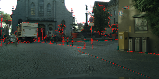
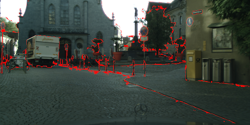
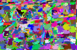
For further analysis, we visualize intermediate clustering results and a predicted mask using HCFormer with Swin-L in Fig. 5. From the visualization of undersegmentation error [51], we find that the model groups pixels well except for the boundaries in intermediate clustering, but it misclassifies clusters for the small objects in this image (e.g., poles and persons in the center). HCFormer cannot extract semantically discriminative features for such small objects, although the obtained features are discriminative in terms of clustering. Thus, to solve errors for the small objects, we may improve the transformer decoder or stack more layers on the backbone for the coarsest scale. We believe that this analysis plays one of the roles in interpretability, and conventional models do not allow for this type of analysis. We present further results and analysis on other datasets in Appendix F.4.
4.3 Ablation Study
To investigate the effect of the hierarchical level and the more effective architecture, we evaluate PQ, FLOPs, and the number of parameters of our model with various hierarchical levels and different numbers of transformer decoder layers. We use the COCO dataset and the ResNet-50 backbone for evaluation. The additional ablation study can be found in Appendix F.3.
| Hierarchical Level | 0 | 1 | 2 | 3 |
|---|---|---|---|---|
| PQ | 41.9 | 45.6 | 46.7 | 47.7 |
| FLOPs | 82G | 83G | 84G | 87G |
| #Params | 37M | 38M | 38M | 38M |
| #Decoder Layers | 1 | 2 | 4 | 8 | 16 |
|---|---|---|---|---|---|
| PQ | 42.0 | 44.8 | 46.7 | 47.7 | 48.0 |
| FLOPs | 85G | 85G | 86G | 87G | 90G |
| #Params | 27M | 29M | 32M | 38M | 51M |
The results are shown in Tabs. 5 and 6. The higher the hierarchical level, the higher the resolution of the predicted masks, increasing PQ and FLOPs. The hierarchical level of 2 would be preferred regarding the balance between accuracy and computational costs in practice, though we adopt the hierarchical level of 3 in Sec. 4.2. In particular, PQ in our model is still comparable to that of MaskFormer [11] even when the hierarchical level is 2.
5 Limitations
HCFormer accomplishes the hierarchical clustering framework by removing the pixel decoder before the segmentation head. However, we do not argue that the pixel decoder is useless, especially in improving segmentation accuracy. Mask2Former uses the multi-scale feature maps obtained from the pixel decoder in the transformer decoder, significantly improving the segmentation accuracy. Also, there are many techniques leveraging the pixel decoder to improve segmentation accuracy [36, 30, 63, 8]. Thus, one of the limitations of HCFormer is that it cannot take advantage of existing techniques using the pixel decoder to improve the segmentation accuracy. This limitation causes the gap between the accuracy of HCFormer and Mask2Former. We will explore alternatives to the modules leveraging the pixel decoder to improve the accuracy in future work.
6 Conclusion
We proposed an attention-based clustering module easily incorporated into existing backbone models, such as ResNet and Swin Transformer. As a result, we accomplished image segmentation via hierarchical clustering in deep neural networks and simplified the segmentation architecture design by removing the pixel decoder before the segmentation head. In experiments, we verified that our method achieves comparable or better accuracy than baseline methods for semantic, instance, and panoptic segmentation. Since our hierarchical clustering allows interpretation, visualization, and evaluation of the intermediate results, we believe that the hierarchical clustering strategy enhances the interpretability of the segmentation models.
References
- [1] Radhakrishna Achanta, Appu Shaji, Kevin Smith, Aurelien Lucchi, Pascal Fua, and Sabine Süsstrunk. SLIC superpixels compared to state-of-the-art superpixel methods. IEEE transactions on pattern analysis and machine intelligence, 34(11):2274–2282, 2012.
- [2] Jimmy Lei Ba, Jamie Ryan Kiros, and Geoffrey E Hinton. Layer normalization. arXiv preprint arXiv:1607.06450, 2016.
- [3] Vijay Badrinarayanan, Alex Kendall, and Roberto Cipolla. Segnet: A deep convolutional encoder-decoder architecture for image segmentation. IEEE transactions on pattern analysis and machine intelligence, 39(12):2481–2495, 2017.
- [4] Irwan Bello. Lambdanetworks: Modeling long-range interactions without attention. arXiv preprint arXiv:2102.08602, 2021.
- [5] Nicolas Carion, Francisco Massa, Gabriel Synnaeve, Nicolas Usunier, Alexander Kirillov, and Sergey Zagoruyko. End-to-end object detection with transformers. In European conference on computer vision, pages 213–229. Springer, 2020.
- [6] Liang-Chieh Chen, George Papandreou, Iasonas Kokkinos, Kevin Murphy, and Alan L Yuille. Deeplab: Semantic image segmentation with deep convolutional nets, atrous convolution, and fully connected crfs. IEEE transactions on pattern analysis and machine intelligence, 40(4):834–848, 2017.
- [7] Liang-Chieh Chen, George Papandreou, Florian Schroff, and Hartwig Adam. Rethinking atrous convolution for semantic image segmentation. arXiv preprint arXiv:1706.05587, 2017.
- [8] Liang-Chieh Chen, Yukun Zhu, George Papandreou, Florian Schroff, and Hartwig Adam. Encoder-decoder with atrous separable convolution for semantic image segmentation. In Proceedings of the European conference on computer vision (ECCV), pages 801–818, 2018.
- [9] Bowen Cheng, Maxwell D Collins, Yukun Zhu, Ting Liu, Thomas S Huang, Hartwig Adam, and Liang-Chieh Chen. Panoptic-deeplab: A simple, strong, and fast baseline for bottom-up panoptic segmentation. In Proceedings of the IEEE/CVF conference on computer vision and pattern recognition, pages 12475–12485, 2020.
- [10] Bowen Cheng, Ishan Misra, Alexander G. Schwing, Alexander Kirillov, and Rohit Girdhar. Masked-attention mask transformer for universal image segmentation. CVPR, 2022.
- [11] Bowen Cheng, Alex Schwing, and Alexander Kirillov. Per-pixel classification is not all you need for semantic segmentation. volume 34, 2021.
- [12] Marius Cordts, Mohamed Omran, Sebastian Ramos, Timo Rehfeld, Markus Enzweiler, Rodrigo Benenson, Uwe Franke, Stefan Roth, and Bernt Schiele. The cityscapes dataset for semantic urban scene understanding. In Proc. of the IEEE Conference on Computer Vision and Pattern Recognition (CVPR), 2016.
- [13] Camille Couprie, Clément Farabet, Laurent Najman, and Yann LeCun. Indoor semantic segmentation using depth information. arXiv preprint arXiv:1301.3572, 2013.
- [14] Jifeng Dai, Kaiming He, and Jian Sun. Convolutional feature masking for joint object and stuff segmentation. In Proceedings of the IEEE conference on computer vision and pattern recognition, pages 3992–4000, 2015.
- [15] Jifeng Dai, Kaiming He, and Jian Sun. Instance-aware semantic segmentation via multi-task network cascades. In Proceedings of the IEEE conference on computer vision and pattern recognition, pages 3150–3158, 2016.
- [16] Bert De Brabandere, Davy Neven, and Luc Van Gool. Semantic instance segmentation with a discriminative loss function. arXiv preprint arXiv:1708.02551, 2017.
- [17] Alexey Dosovitskiy, Lucas Beyer, Alexander Kolesnikov, Dirk Weissenborn, Xiaohua Zhai, Thomas Unterthiner, Mostafa Dehghani, Matthias Minderer, Georg Heigold, Sylvain Gelly, et al. An image is worth 16x16 words: Transformers for image recognition at scale. arXiv preprint arXiv:2010.11929, 2020.
- [18] Clement Farabet, Camille Couprie, Laurent Najman, and Yann LeCun. Learning hierarchical features for scene labeling. IEEE transactions on pattern analysis and machine intelligence, 35(8):1915–1929, 2012.
- [19] Kaiming He, Georgia Gkioxari, Piotr Dollár, and Ross Girshick. Mask R-CNN. In Proceedings of the IEEE international conference on computer vision, pages 2961–2969, 2017.
- [20] Kaiming He, Xiangyu Zhang, Shaoqing Ren, and Jian Sun. Deep residual learning for image recognition. In Proceedings of the IEEE conference on computer vision and pattern recognition, pages 770–778, 2016.
- [21] Shengfeng He, Rynson WH Lau, Wenxi Liu, Zhe Huang, and Qingxiong Yang. Supercnn: A superpixelwise convolutional neural network for salient object detection. International journal of computer vision, 115(3):330–344, 2015.
- [22] Shihua Huang, Zhichao Lu, Ran Cheng, and Cheng He. Fapn: Feature-aligned pyramid network for dense image prediction. In Proceedings of the IEEE/CVF International Conference on Computer Vision, pages 864–873, 2021.
- [23] Varun Jampani, Deqing Sun, Ming-Yu Liu, Ming-Hsuan Yang, and Jan Kautz. Superpixel sampling networks. In Proceedings of the European Conference on Computer Vision (ECCV), pages 352–368, 2018.
- [24] Tommi Kerola, Jie Li, Atsushi Kanehira, Yasunori Kudo, Alexis Vallet, and Adrien Gaidon. Hierarchical lovász embeddings for proposal-free panoptic segmentation. In Proceedings of the IEEE/CVF Conference on Computer Vision and Pattern Recognition, pages 14413–14423, 2021.
- [25] Alexander Kirillov, Ross Girshick, Kaiming He, and Piotr Dollár. Panoptic feature pyramid networks. In Proceedings of the IEEE/CVF Conference on Computer Vision and Pattern Recognition, pages 6399–6408, 2019.
- [26] Alexander Kirillov, Kaiming He, Ross Girshick, Carsten Rother, and Piotr Dollár. Panoptic segmentation. In Proceedings of the IEEE/CVF Conference on Computer Vision and Pattern Recognition, pages 9404–9413, 2019.
- [27] Alexander Kirillov, Evgeny Levinkov, Bjoern Andres, Bogdan Savchynskyy, and Carsten Rother. Instancecut: from edges to instances with multicut. In Proceedings of the IEEE Conference on Computer Vision and Pattern Recognition, pages 5008–5017, 2017.
- [28] Shu Kong and Charless C Fowlkes. Recurrent pixel embedding for instance grouping. In Proceedings of the IEEE Conference on Computer Vision and Pattern Recognition, pages 9018–9028, 2018.
- [29] Hanchao Li, Pengfei Xiong, Jie An, and Lingxue Wang. Pyramid attention network for semantic segmentation. arXiv preprint arXiv:1805.10180, 2018.
- [30] Xiangtai Li, Ansheng You, Zhen Zhu, Houlong Zhao, Maoke Yang, Kuiyuan Yang, Shaohua Tan, and Yunhai Tong. Semantic flow for fast and accurate scene parsing. In European Conference on Computer Vision, pages 775–793. Springer, 2020.
- [31] Yi Li, Haozhi Qi, Jifeng Dai, Xiangyang Ji, and Yichen Wei. Fully convolutional instance-aware semantic segmentation. In Proceedings of the IEEE conference on computer vision and pattern recognition, pages 2359–2367, 2017.
- [32] Yanwei Li, Hengshuang Zhao, Xiaojuan Qi, Liwei Wang, Zeming Li, Jian Sun, and Jiaya Jia. Fully convolutional networks for panoptic segmentation. In Proceedings of the IEEE/CVF Conference on Computer Vision and Pattern Recognition, pages 214–223, 2021.
- [33] Zhiqi Li, Wenhai Wang, Enze Xie, Zhiding Yu, Anima Anandkumar, Jose M Alvarez, Ping Luo, and Tong Lu. Panoptic segformer: Delving deeper into panoptic segmentation with transformers. In Proceedings of the IEEE/CVF Conference on Computer Vision and Pattern Recognition, pages 1280–1289, 2022.
- [34] Xiaodan Liang, Yunchao Wei, Xiaohui Shen, Zequn Jie, Jiashi Feng, Liang Lin, and Shuicheng Yan. Reversible recursive instance-level object segmentation. In Proceedings of the IEEE Conference on Computer Vision and Pattern Recognition, pages 633–641, 2016.
- [35] Huaijia Lin, Xiaojuan Qi, and Jiaya Jia. Agss-vos: Attention guided single-shot video object segmentation. In Proceedings of the IEEE/CVF International Conference on Computer Vision, pages 3949–3957, 2019.
- [36] Tsung-Yi Lin, Piotr Dollár, Ross Girshick, Kaiming He, Bharath Hariharan, and Serge Belongie. Feature pyramid networks for object detection. In Proceedings of the IEEE conference on computer vision and pattern recognition, pages 2117–2125, 2017.
- [37] Tsung-Yi Lin, Michael Maire, Serge Belongie, James Hays, Pietro Perona, Deva Ramanan, Piotr Dollár, and C Lawrence Zitnick. Microsoft coco: Common objects in context. In European conference on computer vision, pages 740–755. Springer, 2014.
- [38] Ze Liu, Yutong Lin, Yue Cao, Han Hu, Yixuan Wei, Zheng Zhang, Stephen Lin, and Baining Guo. Swin transformer: Hierarchical vision transformer using shifted windows. In Proceedings of the IEEE/CVF International Conference on Computer Vision, pages 10012–10022, 2021.
- [39] Jonathan Long, Evan Shelhamer, and Trevor Darrell. Fully convolutional networks for semantic segmentation. In Proceedings of the IEEE conference on computer vision and pattern recognition, pages 3431–3440, 2015.
- [40] Ilya Loshchilov and Frank Hutter. Decoupled weight decay regularization. arXiv preprint arXiv:1711.05101, 2017.
- [41] Wenjie Luo, Yujia Li, Raquel Urtasun, and Richard Zemel. Understanding the effective receptive field in deep convolutional neural networks. Advances in neural information processing systems, 29, 2016.
- [42] Fausto Milletari, Nassir Navab, and Seyed-Ahmad Ahmadi. V-net: Fully convolutional neural networks for volumetric medical image segmentation. In 2016 fourth international conference on 3D vision (3DV), pages 565–571. IEEE, 2016.
- [43] Christoph Molnar. Interpretable machine learning. Lulu. com, 2020.
- [44] Davy Neven, Bert De Brabandere, Marc Proesmans, and Luc Van Gool. Instance segmentation by jointly optimizing spatial embeddings and clustering bandwidth. In Proceedings of the IEEE/CVF Conference on Computer Vision and Pattern Recognition, pages 8837–8845, 2019.
- [45] Adam Paszke, Sam Gross, Francisco Massa, Adam Lerer, James Bradbury, Gregory Chanan, Trevor Killeen, Zeming Lin, Natalia Gimelshein, Luca Antiga, Alban Desmaison, Andreas Kopf, Edward Yang, Zachary DeVito, Martin Raison, Alykhan Tejani, Sasank Chilamkurthy, Benoit Steiner, Lu Fang, Junjie Bai, and Soumith Chintala. Pytorch: An imperative style, high-performance deep learning library. In H. Wallach, H. Larochelle, A. Beygelzimer, F. d'Alché-Buc, E. Fox, and R. Garnett, editors, Advances in Neural Information Processing Systems 32, pages 8024–8035. Curran Associates, Inc., 2019.
- [46] Pedro O Pinheiro, Tsung-Yi Lin, Ronan Collobert, and Piotr Dollár. Learning to refine object segments. In European conference on computer vision, pages 75–91. Springer, 2016.
- [47] Zhen Qin, Weixuan Sun, Hui Deng, Dongxu Li, Yunshen Wei, Baohong Lv, Junjie Yan, Lingpeng Kong, and Yiran Zhong. cosformer: Rethinking softmax in attention. arXiv preprint arXiv:2202.08791, 2022.
- [48] Xiaofeng Ren and Jitendra Malik. Learning a classification model for segmentation. In Computer Vision, IEEE International Conference on, volume 2, pages 10–10. IEEE Computer Society, 2003.
- [49] Olaf Ronneberger, Philipp Fischer, and Thomas Brox. U-net: Convolutional networks for biomedical image segmentation. In International Conference on Medical image computing and computer-assisted intervention, pages 234–241. Springer, 2015.
- [50] Zhuoran Shen, Mingyuan Zhang, Haiyu Zhao, Shuai Yi, and Hongsheng Li. Efficient attention: Attention with linear complexities. In Proceedings of the IEEE/CVF Winter Conference on Applications of Computer Vision, pages 3531–3539, 2021.
- [51] David Stutz, Alexander Hermans, and Bastian Leibe. Superpixels: An evaluation of the state-of-the-art. Computer Vision and Image Understanding, 166:1–27, 2018.
- [52] Teppei Suzuki. Superpixel segmentation via convolutional neural networks with regularized information maximization. In ICASSP 2020-2020 IEEE International Conference on Acoustics, Speech and Signal Processing (ICASSP), pages 2573–2577. IEEE, 2020.
- [53] Teppei Suzuki. Implicit integration of superpixel segmentation into fully convolutional networks. arXiv preprint arXiv:2103.03435, 2021.
- [54] Teppei Suzuki, Shuichi Akizuki, Naoki Kato, and Yoshimitsu Aoki. Superpixel convolution for segmentation. In 2018 25th IEEE International Conference on Image Processing (ICIP), pages 3249–3253. IEEE, 2018.
- [55] Shota Takayama, Teppei Suzuki, Yoshimitsu Aoki, Sho Isobe, and Makoto Masuda. Tracking people in dense crowds using supervoxels. In 2016 12th International Conference on Signal-Image Technology Internet-Based Systems (SITIS), pages 532–537, 2016.
- [56] Jasper RR Uijlings, Koen EA Van De Sande, Theo Gevers, and Arnold WM Smeulders. Selective search for object recognition. International journal of computer vision, 104(2):154–171, 2013.
- [57] Ashish Vaswani, Prajit Ramachandran, Aravind Srinivas, Niki Parmar, Blake Hechtman, and Jonathon Shlens. Scaling local self-attention for parameter efficient visual backbones. In Proceedings of the IEEE/CVF Conference on Computer Vision and Pattern Recognition, pages 12894–12904, 2021.
- [58] Ashish Vaswani, Noam Shazeer, Niki Parmar, Jakob Uszkoreit, Llion Jones, Aidan N Gomez, Łukasz Kaiser, and Illia Polosukhin. Attention is all you need. Advances in neural information processing systems, 30, 2017.
- [59] Huiyu Wang, Yukun Zhu, Hartwig Adam, Alan Yuille, and Liang-Chieh Chen. MaX-DeepLab: End-to-end panoptic segmentation with mask transformers. In Proceedings of the IEEE/CVF Conference on Computer Vision and Pattern Recognition, pages 5463–5474, 2021.
- [60] Wenhai Wang, Enze Xie, Xiang Li, Deng-Ping Fan, Kaitao Song, Ding Liang, Tong Lu, Ping Luo, and Ling Shao. Pyramid vision transformer: A versatile backbone for dense prediction without convolutions. In Proceedings of the IEEE/CVF International Conference on Computer Vision, pages 568–578, 2021.
- [61] Xinlong Wang, Rufeng Zhang, Tao Kong, Lei Li, and Chunhua Shen. Solov2: Dynamic and fast instance segmentation. Advances in Neural information processing systems, 33:17721–17732, 2020.
- [62] Zbigniew Wojna, Vittorio Ferrari, Sergio Guadarrama, Nathan Silberman, Liang-Chieh Chen, Alireza Fathi, and Jasper Uijlings. The devil is in the decoder. In British Machine Vision Conference 2017, BMVC 2017, pages 1–13. BMVA Press, 2017.
- [63] Enze Xie, Wenhai Wang, Zhiding Yu, Anima Anandkumar, Jose M Alvarez, and Ping Luo. Segformer: Simple and efficient design for semantic segmentation with transformers. Advances in Neural Information Processing Systems, 34, 2021.
- [64] Yuwen Xiong, Renjie Liao, Hengshuang Zhao, Rui Hu, Min Bai, Ersin Yumer, and Raquel Urtasun. Upsnet: A unified panoptic segmentation network. In Proceedings of the IEEE/CVF Conference on Computer Vision and Pattern Recognition, pages 8818–8826, 2019.
- [65] Yunyang Xiong, Zhanpeng Zeng, Rudrasis Chakraborty, Mingxing Tan, Glenn Fung, Yin Li, and Vikas Singh. Nyströmformer: A nystöm-based algorithm for approximating self-attention. In Proceedings of the… AAAI Conference on Artificial Intelligence. AAAI Conference on Artificial Intelligence, volume 35, page 14138. NIH Public Access, 2021.
- [66] Jiarui Xu, Shalini De Mello, Sifei Liu, Wonmin Byeon, Thomas Breuel, Jan Kautz, and Xiaolong Wang. Groupvit: Semantic segmentation emerges from text supervision. In Proceedings of the IEEE/CVF Conference on Computer Vision and Pattern Recognition, pages 18134–18144, 2022.
- [67] Fengting Yang, Qian Sun, Hailin Jin, and Zihan Zhou. Superpixel segmentation with fully convolutional networks. In Proceedings of the IEEE/CVF Conference on Computer Vision and Pattern Recognition, pages 13964–13973, 2020.
- [68] Jian Yao, Marko Boben, Sanja Fidler, and Raquel Urtasun. Real-time coarse-to-fine topologically preserving segmentation. In Proceedings of the IEEE conference on computer vision and pattern recognition, pages 2947–2955, 2015.
- [69] Fisher Yu and Vladlen Koltun. Multi-scale context aggregation by dilated convolutions. arXiv preprint arXiv:1511.07122, 2015.
- [70] Qihang Yu, Huiyu Wang, Dahun Kim, Siyuan Qiao, Maxwell Collins, Yukun Zhu, Hartwig Adam, Alan Yuille, and Liang-Chieh Chen. Cmt-deeplab: Clustering mask transformers for panoptic segmentation. In Proceedings of the IEEE/CVF Conference on Computer Vision and Pattern Recognition, pages 2560–2570, 2022.
- [71] Wenwei Zhang, Jiangmiao Pang, Kai Chen, and Chen Change Loy. K-Net: Towards unified image segmentation. Advances in Neural Information Processing Systems, 34, 2021.
- [72] Hengshuang Zhao, Jianping Shi, Xiaojuan Qi, Xiaogang Wang, and Jiaya Jia. Pyramid scene parsing network. In Proceedings of the IEEE conference on computer vision and pattern recognition, pages 2881–2890, 2017.
- [73] Bolei Zhou, Hang Zhao, Xavier Puig, Tete Xiao, Sanja Fidler, Adela Barriuso, and Antonio Torralba. Semantic understanding of scenes through the ade20k dataset. International Journal of Computer Vision, 127(3):302–321, 2019.
- [74] Xizhou Zhu, Han Hu, Stephen Lin, and Jifeng Dai. Deformable convnets v2: More deformable, better results. In Proceedings of the IEEE/CVF Conference on Computer Vision and Pattern Recognition, pages 9308–9316, 2019.
Appendix A Detailed derivation of Eq. (2)
Let be an -dimensional vector fed into the softmax function, which corresponds to a row of in eq. (1), and then -th output of with scale is:
| (6) |
We define and modify eq. (6) as follows:
| (7) |
where . For numerical calculations, when , if , and if . In this case, eq. (6) is equivalent to the following problem:
| (8) |
The solution of this problem is a one-hot vector that holds . By considering eq. (2) for each row, eq. (2) is equivalent to eq. (8). Hence, when , eq. (1) is equivalent to eq. (3).
Appendix B Example PyTorch implementation
We show example PyTorch [45] implementation of the proposed clustering and decoding with the local attention in Listings LABEL:list:clst and LABEL:list:dec. We can easily implement the local attention by using the unfold and einsum functions.
Appendix C Difference between the transformer decoders of HCFormer and Mask2Former
 |
 |
| (a) MaskFormer | (b) Mask2Former |

(c) HCFormer
Mask2Former feeds the Multi-scale feature maps obtained from the pixel decoder into the transformer decoder, unlike MaskFormer and HCFormer. The difference between HCFormer and MaskFormer is only the decoding process, but the difference between HCFormer and Mask2Former is, in addition to the decoding process, the inputs to the transformer decoder. Therefore, in terms of the architecture design, we believe HCFormer is built on MaskFormer rather than Mask2Former.
In our experiments, the accuracy of HCFormer is inferior to that of Mask2Former. However, the PQ of HCFormer is comparable to that of Mask2Former without using multi-scale feature maps in the transformer decoder (i.e., the input to the transformer decoder is the same for both HCFormer and Mask2Former), as shown in Tab. I.
| Mask2Former [10] | HCFormer+ | |
|---|---|---|
| PQ | 50.2 | 50.2 |
| FLOPs | 213G | 96G |
This result indicates HCFormer is not inferior to Mask2Former, and the gap of PQ would be due to the transformer decoder design.
In addition, we report PQ of Mask2Former replacing the well-designed pixel decoder with a simple pixel decoder, FPN [36], in Tab. II.
| Mask2Former [10] | HCFormer+ | |
|---|---|---|
| PQ | 50.7 | 50.2 |
| FLOPs | 226G | 96G |
FPN is one of the most simple pixel decoders used in MaskFormer [11] and K-Net [71]. This replacement reduces the PQ of Mask2Former from 51.9 to 50.7.
As seen in Tabs. I and II, the pixel decoder contributes the improvement of PQ. There are some effective pixel decoder architectures and techniques leveraging the pixel decoder (e.g., the use of multi-scale feature maps as in Mask2Former) to improve the accuracy. Thus, removing the pixel decoder makes the segmentation pipeline simple and interpretable but may lose some means to improve the segmentation accuracy, which is one of the limitations of HCFormer.
Appendix D Detailed experimental setup
We trained models with the Swin-L backbones for the COCO dataset on 4 NVIDIA A100 GPUs and the other models on 2 NVIDIA RTX8000 GPUs. The training protocol follows Mask2Former [10] except for the number of training epochs for HCFormer+. We describe the details as follows.
D.1 Panoptic and instance segmentation on COCO
For HCFormer with the ResNet-50 and Swin-S backbones, we set the number of training epochs and the trainable queries that are fed into the transformer decoder to 50 and 100, respectively. For HCFormer with the Swin-L backbone, these parameters are set to 100 and 200. For HCFormer+, the number of epochs is set to 100 for the ResNet-50 and Swin-S backbones and 200 for the Swin-L backbone, and other parameters are the same as HCFormer. We use an initial learning rate of 0.0001 and a weight decay of 0.05 for all backbones. A learning rate multiplier of 0.1 is applied to the backbone, and we decay the learning rate at 0.9 and 0.95 fractions of the total number of training steps by a factor of 10. We use AdamW optimizer [40] with a batch size of 16. We initialize the scale parameter with 0.1. For data augmentation, we use the same policy as in Mask2Former [10]. For inference, we use the Mask R-CNN inference setting [19], where we resize an image with a shorter side to 800 and a longer side up to 1333.
D.2 Semantic segmentation on AD20K and Cityscapes
We use AdamW [40] and the poly learning rate schedule with an initial learning rate of 0.0001 and a weight decay of 0.05. A learning rate multiplier of 0.1 is applied to the backbones. A batch size is set to 16. We initialize the scale parameter with 0.1. For data augmentation, we use random scale jittering between 0.5 and 2.0, random horizontal flipping, random cropping, and random color jittering. For the ADE20K dataset, if not stated otherwise, we use a crop size of 512512 and train HCFormer for 160k iterations and HCFormer+ for 320k iterations. For the Cityscapes dataset, we use a crop size of 5121024 and train HCFormer for 90k iterations and HCFormer+ for 180k iterations. The number of trainable queries is set to 100 for all models and both datasets.
Appendix E Post-processing for the MaskFormer’s segmentation head and the relation to the clustering
Let be the class probability for masks computed by eq. (4). For a post-processing, we assign a pixel at to one of the predicted probability-assignment pairs via , where denotes the no object class and is the most likely class label, , for each probability-assignment pair . Note that denotes the decoded masks (i.e., ).
The maximization problem in post-processing, , is equivalent to the clustering problem, eq. (2). Specifically, is a similarity between the -th mask query and the pixel at , and the maximization problem selects the most similar mask query. This procedure is the clustering problem for pixels with the mask queries as a prototype. Thus, we can view MaskFormer’s segmentation head as one of the clustering modules.
Appendix F Additional results
F.1 Per-pixel classification with hierarchical clustering
The per-pixel classification head, which is the segmentation head used in many semantic segmentation models, can also be viewed from the clustering perspective. In this head, the weight of the linear classifier with the softmax activation that produces class probability can be viewed as a set of class prototypes. The linear classifier groups pixels based on the class prototypes with the inner product as the similarity. Specifically, let be a weight matrix of the linear classifier, which corresponds to the -class prototypes with -dimensional features, and let be a feature map with pixels. Then, the per-pixel classification models classify pixels as , which is the same formula as the attention in eq. (1) (the norm of can be viewed as the inverse of the scale parameter ). Therefore, we can also view this as the soft clustering problem and naturally incorporate our hierarchical clustering scheme into the per-pixel classification models.
We evaluate our method using the per-pixel classification model. As a baseline, we use FCN-32s [36], FPN [36], PSPNet [72], and Deeplabv3 [7], and we combine the proposed module with FCN-32s, PSPNet, and Deeplabv3. We refer to the combined models as HC-FCN-32s, HC-PSPNet, and HC-Deeplabv3, respectively. We use ResNet-101 [20] as the backbone for all models. Note that PSPNet and Deeplabv3 use dilated convolution [69, 6] in the backbone, and their output stride is 8, meaning that the number of downsampling layers in the backbone is 3. HC-PSPNet and HC-Deeplabv3 use the same backbone architecture as FCN-32s; their output stride is 32. The training protocol follows [72]. We set the crop size for ADE20K to 512512.
| Models | mIoU | Pixel Acc. | msec/image |
|---|---|---|---|
| PSPNet | 42.7 | 80.9 | 48.7 |
| \hdashlineHC-PSPNet | 42.6 | 80.9 | 19.0 |
| Deeplabv3 | 42.7 | 81.0 | 62.5 |
| \hdashlineHC-Deeplabv3 | 42.8 | 81.1 | 22.5 |
| Method | mIoU | Pixel acc. | msec/image |
|---|---|---|---|
| FCN-32s | 71.7 | 94.9 | 71.7 |
| FPN | 75.1 | 95.8 | 82.0 |
| \hdashlineHC-FCN-32s | 76.1 | 96.1 | 87.2 |
| PSPNet | 77.7 | 96.2 | 298.7 |
| \hdashlineHC-PSPNet | 77.6 | 96.2 | 88.1 |
| Deeplabv3 | 78.4 | 96.3 | 380.8 |
| \hdashlineHC-Deeplabv3 | 77.6 | 96.3 | 93.9 |
We show the evaluation results for the validation set in Tab. III. The latency of HC-PSPNet and HC-Deeplabv3 is lower than that of PSPNet and Deeplabv3, and HC-PSPNet shows a comparable result for PSPNet for both datasets. However, mIoU of HC-Deeplabv3 on Cityscapes is lower than that of Deeplabv3. Deeplabv3 uses atrous spatial pyramid pooling (ASPP) that uses several dilated (atrous) convolution layers with different dilation, and the maximum dilation is 24, which corresponds to the convolution with a kernel size of 49. For HC-Deeplabv3, the resolution of the feature map fed into the ASPP layer would be quite low. As a result, HC-Deeplabv3 degrades mIoU from Deeplabv3.
Compared to FCN-32s, HC-FCN-32s significantly improves mIoU because it can preserve detailed information, such as object boundaries, via the clustering module. In addition, HC-FCN-32s shows a superior mIoU than FPN, that is, FCN-32s with the simple pixel decoder, which is also used in MaskFormer [11], while the latency is higher than FPN. This result is consistent with the results of the comparison between HCFormer and MaskFormer.
F.2 Effect of downsampling modules
In the experiments, we use the deformable convolution v2 (DCNv2) [74] as the downsampling for the ResNet backbone. We verify its effect by comparing the ResNet backbone with and without DCNv2. We train models using the same training protocol for both models with and without DCNv2 (Sec. D.1).

We show the evaluation results for COCO [37] in Tab. IV. Note that the hierarchical level is shown in Fig. II. Since the downsampling layer is replaced with DCNv2 only for the layers to which the clustering module is attached, both results for the hierarchical level of 0 are the same. DCNv2 significantly improves PQ, especially for hierarchical levels of 2 and 3. The higher the hierarchical level, the more sampling error is accumulated. Thus, the improvement is larger for the higher level.
|
|
||||||||||||||||||||||||||||||||||||||||
| (a) w/ DCNv2 | (b) w/o DCNv2 |
Note that we do not use DCNv2 as downsampling for the transformer-based backbone (Swin-S and Swin-L), and the accuracy of HCFormer with the transformer-based backbone is higher than that of MaskFormer. Thus, the effectiveness of HCFormer is significant, although its accuracy of HCFormer with the CNN-based backbone is almost the same as that of MaskFormer.
F.3 Additional ablation study
We show the additional ablation study. Basically, we use ResNet-50 as a backbone model, except for the result in Tab. VIII, and the training protocol is the same as described in Sec. D.
We evaluate HCFormer with the transformer decoder used in MaskFormer [11], although the masked transformer decoder [10] was used in the experiments in the main manuscript. As shown in Tab. V, HCFormer with the standard transformer decoder still outperforms MaskFormer even though the DCNv2 is not used. The difference between HCFormer w/o DCNv2 and MaskFormer in Tab. V is the segmentation process: MaskFormer generates segmentation masks directly from the per-pixel features, and HCFormer generates them based on the hierarchical strategy. This indicates that our hierarchical clustering scheme generates more accurate masks than direct inference from the per-pixel features.
| method | PQ | FLOPs |
| MaskFormer [11] | 46.5 | 181G |
| Mask2Former [10] | 47.1 | 213G |
| \hdashlineHCFormer w/o DCNv2 | 46.8 | 97G |
| HCFormer w/ DCNv2 | 47.6 | 97G |
We also show the results of Mask2Former without the masked attention in the transformer decoder. PQ of HCFormer without DCNv2 is slightly worse than that of Mask2Former, but we believe that due to the use of multi-scale feature maps, as described in Sec. C.
| #Queries | 20 | 50 | 100 | 150 | 200 |
|---|---|---|---|---|---|
| COCO (PQ) | 42.2 | 46.3 | 47.7 | 47.9 | 47.9 |
| ADE20K (mIoU) | 44.4 | 45.5 | 45.5 | 44.8 | 44.4 |
| Cityscapes (mIoU) | 75.9 | 75.4 | 76.7 | 76.2 | 76.4 |
| Hierarchical Level | 0 | 1 | 2 | 3 |
|---|---|---|---|---|
| mIoU | 42.2 | 43.4 | 44.0 | 45.5 |
| FLOPs | 28G | 28G | 28G | 29G |
| #Params | 37M | 38M | 38M | 38M |
| Hierarchical Level | 0 | 1 | 2 | 3 |
|---|---|---|---|---|
| PQ | 47.5 | 49.7 | 50.5 | 50.9 |
| FLOPs | 167G | 167G | 168G | 170G |
| #Params | 62M | 62M | 62M | 62M |
| #Decoder Layers | 1 | 2 | 4 | 8 | 16 |
|---|---|---|---|---|---|
| mIoU | 43.2 | 44.4 | 44.5 | 45.5 | 46.1 |
| FLOPs | 28G | 28G | 28G | 29G | 31G |
| #Params | 27M | 29M | 32M | 38M | 51M |
 |
 |
 |
 |
 |
 |
 |
 |
 |
 |
 |
 |
 |
 |
 |
 |
 |
 |
 |
 |
 |
 |
 |
 |
 |
 |
 |
 |
 |
 |
 |
 |
We evaluate HCFormer using a various number of trainable queries (Tab. VI). The segmentation accuracy is saturated at about 100 or 150. For memory efficiency, 50 or 100 queries would be preferred.
We evaluate HCFormer with the various hierarchical levels on the semantic segmentation (ADE20K). We verify the improvement of the accuracy on the semantic segmentation, as shown in Tab. VII. In addition, we evaluate HCFormer with the Swin-S [38] backbone with various numbers of hierarchical levels on COCO [37]. Regardless of the backbone type and dataset, a higher hierarchical level leads to higher accuracy.
We evaluate HCFormer with the ResNet-50 backbone with various numbers of transformer decoder layers on ADE20K. MaskFormer [11] reports reasonable semantic segmentation performance (43.0 mIoU on ADE20K) with only one transformer decoder layer. HCFormer with only one transformer decoder layer also shows reasonable results (43.2 mIoU on ADE20K), as shown in Tab. IX. This result is better than the per-pixel classification baselines with ResNet-101 [20], such as PSPNet [72] and Deeplabv3 [7], as shown in Tab. III. The deeper transformer decoder improves mIoU, and four or eight layers would be sufficient for HCFormer.
F.4 Visualization
We show example results on ADE20K by HCFormer with Swin-L [38] in Fig. III. Basically, the undersegmentation error appears near the boundaries because of ambiguity and downsampling in stem and patch embedding layers of the backbone to which the clustering module is not attached. In the outdoor image (top row), the undersegmentation error appears in the tree region (green region) at the coarser clustering levels, but this would be due to ambiguity in the annotation. In the indoor image (bottom row), the undersegmentation error appears below the cabinet region (pink region) in all the levels because the pixels in the wall and floor regions are grouped. In addition, HCFormer misclassifies the cabinet and the towel as wall and door, respectively. The backbone model would not recognize their semantics, although it was able to discriminate between pixels in the cabinet and pixels in the wall because the undersegmentation error only appears in their boundaries.
We show example results for COCO panoptic segmentation by HCFormer+ with Swin-L [38] in Fig. IV. HCFormer groups pixels in images well, although there are some misclassifications. To solve such a misclassification error, we might need to improve the transformer decoder and/or incorporate stronger backbones.