Harnessing Data for Accelerating Model Predictive Control by Constraint Removal
Abstract
Model predictive control (MPC) solves a receding-horizon optimization problem in real-time, which can be computationally demanding when there are thousands of constraints. To accelerate online computation of MPC, we utilize data to adaptively remove the constraints while maintaining the MPC policy unchanged. Specifically, we design the removal rule based on the Lipschitz continuity of the MPC policy. This removal rule can use the information of historical data according to the Lipschitz constant and the distance between the current state and historical states. In particular, we provide the explicit expression for calculating the Lipschitz constant by the model parameters. Finally, simulations are performed to validate the effectiveness of the proposed method.
I Introduction
Model predictive control (MPC) is a popular optimal control technique and has many successful applications, including autonomous driving [1], industrial process [2], and robotic manipulation [3]. By solving online a receding-horizon optimization problem, the MPC computes the control input in real-time that ensures the satisfaction of system constraints. However, solving an optimization problem per timestep can be computationally demanding even for linear dynamical systems, especially when there are thousands of constraints [4]. Thus, reducing the computation burden has become an important problem for both theoretical and practical researchers.
Manifold approaches to accelerating the online computation include model reduction [5], explicit MPC [6], tailored solvers [7], and constraint removal [8]. Recently, there has been an increasing interest in the constraint removal approach as it can utilize online data to further reduce the computation time [9]. The constraint removal method first pre-determines unnecessary (inactive) constraints of the receding-horizon optimization problem by exploiting local properties of the optimization problem, such as reachable sets [9], region of activity [10], and contraction properties of the cost function [11]. Then, it removes these constraints to reduce the scale of the optimization problem, while maintaining the solution unchanged. Very recently, Nouwens et al. [12] proposes a general system-theoretic principle to design the constraint removal rule using the online closed-loop state-input data, leading to the constraint-adaptive MPC (ca-MPC) framework. While the ca-MPC enables the use of system-theoretic properties (e.g., reachability and optimality), it is conservative as only the data at current time is utilized. In fact, the historical data should also be taken into account in some applications. For example, the racing car routinely runs on the same track, and using data from past iterations may further improve the performance of the constraint-removal method.
In this paper, we propose a new constraint removal method for the ca-MPC of linear systems, which uses the historical state-input data to further accelerate the online computation. Instead of using reachability and optimality of the receding-horizon problem [12], we exploit the Lipschitz continuity of the MPC policy in the state to design the removal rule. However, an explicit Lipschitz constant is challenging to obtain and is absent in the literature. Fortunately, by estimating the KKT solution of the receding-horizon problem, we are able to provide an explicit expression for the Lipschitz constant. In particular, the Lipschitz constant can be computed offline using only the model parameters. By leveraging the Lipschitz continuity, the proposed constraint removal rule can utilize the historical state data that is “close” to the current system state. Finally, simulations are performed to validate the effectiveness of the proposed method.
Our result on the Lipschitz constants of the MPC policy has independent interests of its own. The Lipschitz constant is beneficial in various realization of MPC including robustness against disturbance [13] and neural network-based approximation [14]. However, an explicit Lipschitz constant is challenging to obtain. While recent works estimate the Lipschitz constant via enumerating potential active sets [15] or a mixed-integer linear program [14][16], they are time-consuming and lack an explicit expression. In contrast, we provide the first explicit Lipschitz constant that can be efficiently computed using model parameters.
The rest of this paper is organized as follows. The notation is given in the remainder of this section. Section II introduces the linear MPC and formulates the problem. We provide an explicit expression of the Lipschitz constant and present the ca-MPC scheme in Section III. We illustrate the effectiveness of the proposed scheme with simulation in Section IV and give a conclusion in Section V.
Notation. We denote the set of real number by , the set of -dimensional real-valued vectors by and the set of -dimensional real-valued matrices by . Given a matrix , denotes its transpose, denotes its -th row and so is the vector. is the i-th largest eigenvalue of . Specially, we define as the smallest eigenvalue of . For two vectors , we denote element-wise multiplication by . For any set of indices , denotes the submatrix obtained by selecting the rows indicated in . is denoted as the number of elements in the set . . For two sets , we define .
II Problem formulation and background
In this section, we introduce the linear system to be controlled and the linear MPC setup (see Section II-A). Furthermore, we introduce the constraint-adaptive MPC and formulate our problem in Section II-B.
II-A Linear MPC
We consider a discrete-time linear time-invariant (LTI) system:
| (1) |
where and denote the states and the inputs, respectively, at discrete time . and are known system matrices. The system is subject to polyhedral state and input constraints:
| (2) |
where and origin is in the interior of .
Based on the system dynamic (1) and the constraints (2), an MPC over a finite time horizon of length , given the state at time , can be formulated as
| (3) | ||||
| s.t. | ||||
where
| (4) |
Here, denote the predicted state and the predicted input. is composed of the stage cost and the terminal cost where the weights are symmetric positive definite matrices. The constraint is the terminal constraint.
Let be the solution of (3). Then, the first input is applied to the system:
| (5) |
The optimization (3) can be expressed as a standard multiparameter quadratic programming (mp-QP) form by regarding as the parameter vector:
| (6a) | ||||
| s.t. | (6b) | |||
where is the current state, are parameter matrices which are obtained from . We denote an optimal solution to (6) by . The set of indices of the active constraints responding to is denoted by .
If mp-QP has many constraints in (6b), then it is challenging and time-consuming to solve this optimization problem. One approach to reduce computational burden is to remove some redundant constraints.
II-B Constraint-adaptive MPC
Nouwens et al. [12] proposed a online constraint removal framework for linear system, called constraint-adaptive MPC. Specially, his method introduced the reduced MPC problem which have fewer constraints compared to the original MPC problem. The mp-QP version of the reduced MPC problem is formulated as follows:
| (7a) | ||||
| s.t. | (7b) | |||
where we define the mapping from the state space to the indices set of reduced constraints. denote the optimal solution of (7).
To guarantee that the optimal solution to (7) is the same as that to (6), Nouwens et al. [12] build upon the theorem as follows:
Lemma 1 (Theorem 1, [12]).
In Lemma 1, is regarded as the outer approximation of . This approximation can be obtained by some information about the optimal solution (e.g., reachability and optimality [12]).
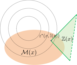
The way to apply the Lemma 1 is to first construct the outer approximation of for all possible choices of . Then, the indices in are selected such that (8b) is satisfied. Finally, constraints in are removed to formulate the reduced mp-QP problem (7). As shown in Fig. 1, is in the half-space formed by and contained by . In this case, the constraints specified by can be removed directly without changing the optimal solution, i.e. . Thus, the design of outer approximation is essential, and a good approximation leads to efficient constraint removal. In this paper, we are interested in the following problem:
Problem 1.
Design an approximation in Lemma 1 and improve the constraints removal.
III Exploiting historical data for ca-MPC
In this section, we use the historical data to design the outer approximation . This is motivated by an observation that the optimal solution for mp-QP is Lipschitz continuous. If the current state is close to the previous state , then the optimal solution of the current state is in a circle centered around that of which radius is . This information can be used to design the outer approximation , then evaluate and remove redundant constraints. Specifically, we provide an explicit form of the Lipschitz constant of linear MPC in Section III-A. Based on this, we design a constraint removal mechanism that utilizes historical data and present our MPC scheme in Section III-B.
III-A The Lipschitz constant of reduced mp-QP
Consider a mp-QP problem with constraints selected by which has no relation with the state x compared to (7):
| (9a) | ||||
| s.t. | (9b) | |||
Here, we denote the optimal solution of (9) by . For each , there exists a [6] such that
| (10) |
The Lipschitz constant depends on . It is hard to compute the Lipschitz constant unless the explicit law is known [15]. In fact, the explicit law is intractable for large-scale system. In our cases, we need to calculate the maximum Lipschitz constant of mp-QP in different , i.e., . As far as we know, no methods can calculate this constant efficiently. To address this problem, we provide an explicit form for with very low computational cost as follows:
Theorem 1.
For any , it holds that
| (11) |
with
| (12) | ||||
Remark 1.
This Lipschitz constant is finite because is positive definite matrix and . Also, this constant can be offline computed from the model parameters.
Theorem 1 provides an efficient computing method for the Lipschitz constant. Its computation includes matrix multiplication and matrix norm. Let us analyze the computation complexity of the matrix norm. Here, we are interested in the mp-QP that exists many constraints, i.e., . For a matrix , its matrix norm . The computation complexity per step of and with power iteration methods are and , respectively. So the computation complexity of is or . The dimensions of three matrix in (12) to compute norm are , and . Although , the computation complexity of matrix norm in (12) is and are not influenced by the number of constraints.
III-B The outer approximation
We now utilize the Theorem 1 to construct the outer approximation . Then, we propose the ca-MPC scheme based on the mapping computed by .
We present the key lemma used in the design of :
Lemma 2.
For any , if , we have
| (14) |
Proof.
Let in Theorem 1:
| (15) |
In Lemma 2, we consider as the current state and as a historical state. Let reduced constraint indices satisfy :
| (18) |
where
| (19) |
Equation (19) indicates that is a sphere set. The term in (19) is the distance between the current state and historical state. This distance is expected to be small so that can be contained in many constraints of . Based on this distance, we can evaluate if the historical state can provide good information for and can help remove some redundant constraints. As a result, the historical data which have the smallest distance is used to design and construct .
To select the removal constraints , we utilize the sphere half-space intersection check to evaluate if the sphere set is entirely constained in the half-space specified by the constraint in . This check leads to our removal rule:
| (20) |
In Algorithm 1, we present the removal process and present our overview of the proposed MPC scheme. Theorem 2 shows that our removal rule (20) maintains the trajectory unchanged.
Theorem 2.
Proof.
We prove this Theorem by induction.
For each , it follows from line 7 that
| (24) |
We know that the distance between and plane is . It follow from (22)(23)(24) that does not intersect with the plane . Also we know . Then . As a result, it holds that
| (25) |
According to Lemma 1, combining (22), (25) with (21) yields
which can complete the proof by induction.
∎
Theorem 2 indicates that our algorithm exploits the historical data to accelerate the optimization without changing the state trajectory. Compared to solving the optimization problem (6) with a large number of constraints, the computation in line 6 of Algorithm 1 is low unless the historical data is very large. Even though this computation is limited by the number of historical data, some techiques can be used to overcome this problem. For example, the redundant data can removed when distance between two historical data is small.
IV Simulations
In this section, we apply the proposed method to the double integrator system. The simulations are conducted in MATLAB.
Consider the double integrator system:
where the input is constrained by . The state constraints are
which are linearly approximated by two quadratic constraints (27). and are the boundary points of
| (27a) | |||
| (27b) | |||
respectively, and
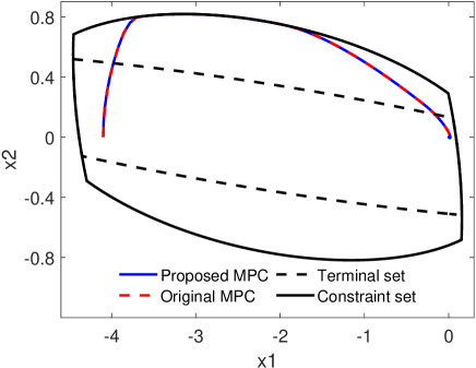
Similarly, the terminal constraint is constructed by piecewise linear approximation of two quadratic constraints (27a) and with . The state constraints and terminal constraint are shown in Fig. 2.
The MPC cost function is defined as (4) where
The prediction horizon is and the total number of constraints is . The Lipschitz constant is calculated by (13) where
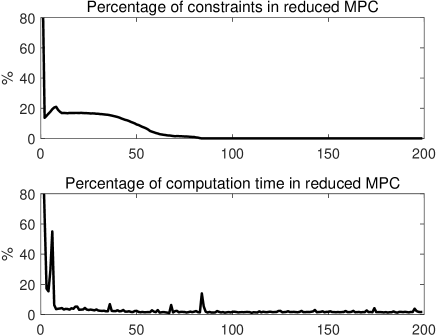
The system is initialized at and expected to converge to the origin under the control policy. The data set is initialized with one data . The resulting state trajectories are shown in Fig. 2. The closed-loop trajectories under the original MPC and the proposed ca-MPC steer towards the origin without violating the constraints. Moreover, our proposed ca-MPC produces the same trajectories as that of the original MPC. The comparation of the constraints number and computation time between two schemes are shown in Fig. 3. After 10 steps, the proposed scheme decreases more than 80% constraints, then the proposed scheme removes almost all of constraints after 80 steps. In addition, our ca-MPC scheme is 10-100 times faster to compute compared to the original MPC scheme.
V Conclusions
In this paper, we presented the constraint-adaptive MPC scheme which can exploit the historical data to remove constraints. A crucial aspect of our method is to analyze the Lipschitz continuity and design the outer approximation. In particular, we provided an explicit form of the Lipschitz constant which can be calculated offline and efficiently. Then, we proved that the closed-loop behavior remains unchanged compared to the original MPC policy. Simulations validated that our scheme can significantly reduce the number of constraints and improve the computational speed.
Appendix A Proof of Theorem 1
The KKT conditions related to the mp-QP (9) are
| (28a) | |||
| (28b) | |||
| (28c) | |||
| (28d) | |||
Solving (28a) for z yields
| (29) |
Let superscript denotes the variable corresponding to active constraints . Without loss of generality, we assume that the rows of are linearly independent [6]. For active constraints, . Combining it with (29):
| (30) |
where correspond to the set of active constraints, and is invertible because the rows of are linearly independent. Substituting (30) into (29):
Define
We obtain
| (31) |
In fact, are the submatrices composed by the rows in respectively. We can represent these matrix with such that
Here, the matrix is non-square matrix that has at most one entry of 1 in each row and each column with all other entries 0. Substituting this into the second term of (31) yields
| (32) | ||||
The last inequation is built with the submultiplicative property of the spectral norm. It follows that
| (33) | ||||
where the second and third equation are satisfied because is positive definite matrix.
is positive definite matrix and can be written as (i.e. Cholesky decomposition) where has full rank. Let The matrices and have the same non-zero eigenvalues and the number of non-zero eigenvalues is :
| (34) |
According to the Corollary in [17, Corollary 4.3.15.], if two matrices are Hermitian, then . As a result,
where can be any element in . The rank of is less than . So its -th largest eigenvalue is zero. Moreover, . We have
| (35) |
References
- [1] G. Cesari, G. Schildbach, A. Carvalho, and F. Borrelli, “Scenario model predictive control for lane change assistance and autonomous driving on highways,” IEEE Intelligent transportation systems magazine, vol. 9, no. 3, pp. 23–35, 2017.
- [2] S. J. Qin and T. A. Badgwell, “A survey of industrial model predictive control technology,” Control engineering practice, vol. 11, no. 7, pp. 733–764, 2003.
- [3] C. M. Best, M. T. Gillespie, P. Hyatt, L. Rupert, V. Sherrod, and M. D. Killpack, “A new soft robot control method: Using model predictive control for a pneumatically actuated humanoid,” IEEE Robotics & Automation Magazine, vol. 23, no. 3, pp. 75–84, 2016.
- [4] J. G. Van Antwerp and R. D. Braatz, “Model predictive control of large scale processes,” Journal of Process Control, vol. 10, no. 1, pp. 1–8, 2000.
- [5] S. Hovland, K. Willcox, and J. T. Gravdahl, “Mpc for large-scale systems via model reduction and multiparametric quadratic programming,” in Proceedings of the 45th IEEE Conference on Decision and Control. IEEE, 2006, pp. 3418–3423.
- [6] A. Bemporad, M. Morari, V. Dua, and E. N. Pistikopoulos, “The explicit linear quadratic regulator for constrained systems,” Automatica, vol. 38, no. 1, pp. 3–20, 2002.
- [7] J. L. Jerez, E. C. Kerrigan, and G. A. Constantinides, “A condensed and sparse qp formulation for predictive control,” in 2011 50th IEEE Conference on Decision and Control and European Control Conference. IEEE, 2011, pp. 5217–5222.
- [8] A. J. Ardakani and F. Bouffard, “Acceleration of umbrella constraint discovery in generation scheduling problems,” IEEE Transactions on Power Systems, vol. 30, no. 4, pp. 2100–2109, 2014.
- [9] S. Nouwens, B. de Jager, M. M. Paulides, and W. M. H. Heemels, “Constraint removal for mpc with performance preservation and a hyperthermia cancer treatment case study,” in 2021 60th IEEE Conference on Decision and Control (CDC). IEEE, 2021, pp. 4103–4108.
- [10] M. Jost and M. Mönnigmann, “Accelerating model predictive control by online constraint removal,” in 52nd IEEE Conference on Decision and Control. IEEE, 2013, pp. 5764–5769.
- [11] M. Jost, G. Pannocchia, and M. Mönnigmann, “Online constraint removal: Accelerating mpc with a lyapunov function,” Automatica, vol. 57, pp. 164–169, 2015.
- [12] S. A. N. Nouwens, M. M. Paulides, and M. Heemels, “Constraint-adaptive mpc for linear systems: A system-theoretic framework for speeding up mpc through online constraint removal,” Automatica, vol. 157, p. 111243, 2023.
- [13] P. O. Scokaert, J. B. Rawlings, and E. S. Meadows, “Discrete-time stability with perturbations: Application to model predictive control,” Automatica, vol. 33, no. 3, pp. 463–470, 1997.
- [14] F. Fabiani and P. J. Goulart, “Reliably-stabilizing piecewise-affine neural network controllers,” IEEE Transactions on Automatic Control, vol. 68, no. 9, pp. 5201–5215, 2023.
- [15] M. S. Darup, M. Jost, G. Pannocchia, and M. Mönnigmann, “On the maximal controller gain in linear mpc,” IFAC-PapersOnLine, vol. 50, no. 1, pp. 9218–9223, 2017.
- [16] D. Teichrib and M. S. Darup, “Efficient computation of lipschitz constants for mpc with symmetries,” in 2023 62nd IEEE Conference on Decision and Control (CDC). IEEE, 2023, pp. 6685–6691.
- [17] R. A. Horn and C. R. Johnson, Matrix analysis. Cambridge university press, 2012.