Halo concentration strengthens dark matter constraints in galaxy-galaxy strong lensing analyses
Abstract
A defining prediction of the cold dark matter (CDM) cosmological model is the existence of a very large population of low-mass haloes. This population is absent in models in which the dark matter particle is warm (WDM). These alternatives can, in principle, be distinguished observationally because halos along the line-of-sight can perturb galaxy-galaxy strong gravitational lenses. Furthermore, the WDM particle mass could be deduced because the cut-off in their halo mass function depends on the mass of the particle. We systematically explore the detectability of low-mass haloes in WDM models by simulating and fitting mock lensed images. Contrary to previous studies, we find that halos are harder to detect when they are either behind or in front of the lens. Furthermore, we find that the perturbing effect of haloes increases with their concentration: detectable haloes are systematically high-concentration haloes, and accounting for the scatter in the mass-concentration relation boosts the expected number of detections by as much as an order of magnitude. Haloes have lower concentration for lower particle masses and this further suppresses the number of detectable haloes beyond the reduction arising from the lower halo abundances alone. Taking these effects into account can make lensing constraints on the value of the mass function cut-off at least an order of magnitude more stringent than previously appreciated.
keywords:
dark matter — gravitational lensing: strong1 Introduction
The nature and identity of dark matter (DM) remain fundamental open questions in contemporary astrophysics; enormous effort is currently being directed at finding the answer. Numerical simulations of the cosmological process of structure formation (e.g. Davis et al., 1985; Springel et al., 2005; Frenk & White, 2012) have shown that a model based on the assumption that the DM consists of cold dark matter (CDM) particles can very successfully reproduce a number of large-scale astrophysical measurements (e.g. Planck Collaboration et al., 2020; Wang et al., 2016; Alam et al., 2017). Several plausible DM candidates behave like CDM on large scales, but luckily, their different physical properties can make them distinguishable on subgalactic scales. The defining property of standard CDM is the nearly scale-invariant primordial power-spectrum of density fluctuations, which results in an equally distinctive halo mass function, characterized by a large population of haloes down to masses comparable to the Earth’s mass (Jenkins et al., 2001; Diemand et al., 2008; Angulo et al., 2012; Green, Hofmann, & Schwarz, 2005; Wang et al., 2020). Most alternative DM models predict a suppression of the primordial power spectrum on small scales and an associated truncation of the halo mass function at a mass, . For example, in the popular warm dark matter (WDM) model, free-streaming arising from the thermal velocities of the particles at early times is the cause of the suppression which occurs at a mass scale that is roughly inversely proportional to the WDM particle mass (e.g. Avila-Reese et al., 2003; Schneider et al., 2012; Lovell et al., 2012; Bose et al., 2016).
Current constraints on the warm DM model stem primarily from a combination of the abundance of satellite galaxies in the Milky Way (Kennedy et al., 2014; Lovell et al., 2012, 2016; Newton et al., 2020) and the properties of the Lyman- forest inferred from high-redshift QSO spectra (Viel et al., 2013; Baur et al., 2016; Iršič et al., 2017). A joint analysis of these, together with constraints from gravitational lensing (see below), place at M⊙ for a thermal WDM relic. These bounds, however, are subject to possible systematics such as uncertainties in the galaxy formation physics in the case of satellites (Newton et al., 2020) and assumptions on the thermal history of the intergalactic medium at high-redshift in the case of the Lyman- forest (e.g. Garzilli, Boyarsky, & Ruchayskiy, 2017; Garzilli et al., 2019). Constraints from independent probes, such as we discuss here, are therefore a priority.
Strong gravitational lensing has emerged as an independent way to quantify the abundance of low-mass DM haloes and thus constrain the WDM particle mass. This technique uses galaxy-galaxy strong gravitational lenses (e.g., Bolton, 2005; Shu et al., 2016) to detect low-mass haloes through the perturbations they cause to the lens image (see also the alternative approach based on flux ratio anomalies of lensed quasars, e.g., Xu et al., 2015; Gilman et al., 2018, 2019, 2020; Harvey et al., 2020). These perturbations make it possible to detect both satellite haloes in the main lens (subhaloes) and low-mass ‘central’ haloes along the line-of-sight (LOS) (Li et al., 2017; Despali et al., 2018), even if they contain negligible baryonic mass. In fact, in the mass range of interest, M⊙, haloes are too small to have made a galaxy and so are completely dark (Benitez-Llambay & Frenk, 2020). This is a great advantage as the abundance and structure of isolated DM haloes is unaffected by complications associated with baryonic processes and is very robustly determined by cosmological simulations. Distortions of strong lenses are therefore an especially clean way to probe the DM particle mass.
A small number of detections have already been claimed, albeit for subhaloes more massive than those that can test WDM models (Vegetti et al., 2010, 2012; Hezaveh et al., 2016). The most challenging aspect of lensing lies in using these detections – and non-detections as well – to extract quantitative inferences about the DM model (e.g. Vegetti et al., 2014, 2018; Ritondale et al., 2019). To do so, it is necessary to formulate robust predictions. For example, how many detections are to be expected in a given lensing system assuming CDM, or as a function of the WDM particle mass?
Quantifying the number of detectable haloes, , in a specific lens means identifying which DM haloes, out of the cosmological population of haloes, can cause ‘observable’ perturbations to that system. More specifically, for a warm DM particle with cutoff mass, ,
| (1) |
where is the cosmological number density of DM haloes111Here we focus on LOS haloes. The same formalism applies to subhaloes in the main lens, albeit with a different density, . at sky-projected location, , redshift, , and with properties, (such as mass, concentration, etc.), while is the probability of actually detecting such haloes were they to be truly present in the observed system, given the properties of the lens itself, , and those of the data – for instance, the noise properties, . In other words, were a halo to be truly present:
-
•
if its perturbations are too small to be observable, implying that a perturbing halo mass component would not be required in the modelling to describe the data;
-
•
if its perturbations make a model including a perturbing mass component statistically preferable to one that does not.
The increase in Bayesian evidence between the two models (or the increase in log-likelihood) is often used as a deciding metric, and most studies (e.g. Vegetti et al., 2014, 2018) have indeed reduced to a binary classification: were the halo to be truly present, , if including a perturbing mass component causes the Bayesian evidence or log-likelihood to increase beyond some given threshold. This is usually referred to as the sensitivity function and, simply put, it identifies the region of parameter space (comprising both physical cosmological volume and halo properties) which can be actually probed by lensing. In contrast to the cosmological number density of DM haloes, , the sensitivity function itself does not directly depend on the DM model222Although it does depend on the density profile of the perturbing haloes, which, in turn, may itself depend on the DM model., but it does shape expectations for the number of detectable haloes, – as well as expectations for any other observable obtained through structure lensing studies.
While advanced tools to model optical strong lensing data have been developed (e.g. Vegetti & Koopmans, 2009; Nightingale et al., 2021), it remains computationally expensive to calculate the sensitivity function and formulate these predictions. Systematic exploration is required to establish the range of properties that make a perturber detectable. A minimum list of the independent variables include the halo mass and halo concentration, the projected location of the halo with respect to the lensing system, and its redshift. In addition, the sensitivity function is unique to each individual lensing system because degeneracies in the lensing effects are such that different lensing configurations can ‘reabsorb’ the perturbations of identical DM haloes with different efficiencies. In practice, mapping the entire parameter space for each lens is often computationally prohibitive, and a number of simplifying assumptions have been used to obtain estimates of the integral in equation (1). Here, we explore the effect of these simplifications. Among the independent variables mentioned above, halo concentration and halo redshift are the most important.
For instance, Minor et al. (2021) has recently shown that the halo concentration must be included as a free parameter when modelling a perturber: if the concentration is fixed, the inferred perturber’s mass may be biased by a factor of up to 6. They also show that higher halo concentrations make perturbers more easily detectable, as the lensing effect of any mass distribution is driven by its surface density. However, the intrinsic scatter in the concentration of DM haloes (e.g. Neto et al., 2007; Ludlow et al., 2016; Wang et al., 2020) has so far been ignored in sensitivity mapping studies; instead, the mass-concentration relation has been collapsed onto the concentration axis entirely, forcing all haloes onto the mean value for their mass. Additionally, the dependence of the mean mass-concentration relation on the DM model itself has also been neglected (e.g. Vegetti et al., 2018; Ritondale et al., 2019). This latter assumption leaves cosmological halo abundances as the single measure to differentiate between WDM models of different particle mass, despite the fact that warmer DM models produce haloes that are increasingly less dense than their equal-mass CDM counterparts (e.g. Lovell et al., 2012; Bose et al., 2016).
As regards the perturber’s redshift, this axis has often been collapsed by adopting a one-to-one scaling relation that recasts a halo’s redshift in terms of its effective mass (Li et al., 2017; Despali et al., 2018). This is obtained by requiring that the lensing convergence – i.e. the strength of the lensing effect – should remain nearly constant. This is not equivalent to performing a full non-linear search, as done on real data, and therefore does not fully take into account the modelling degeneracies that can occur in the real case. Lastly, we also briefly reflect on the influence of noise properties and the role of a specific noise realization.
To explore the parameter space of a sensitivity function fully, we use mock data and models that are somewhat simpler than those employed in state-of-the-art lens modelling studies (e.g. Vegetti & Koopmans, 2009; Nightingale et al., 2019; Powell et al., 2021). Specifically, we use models featuring parametric sources rather than non-parametric pixelized sources (e.g. Warren & Dye, 2003; Dye & Warren, 2005; Birrer, Amara, & Refregier, 2016; Nightingale & Dye, 2015). This allows us to develop and apply a fitting procedure based on a gradient descent algorithm, which is efficient enough to enable the exploration of all of the independent dimensions of the parameter space relevant to this problem. This work compares how previous assumptions regarding the sensitivity function affect the power of strong lensing to discriminate between different DM models, which we assume is not strongly dependent on the specific approach to source modelling.
In this work, we concentrate on LOS isolated perturbers, which we model as pure NFW profiles (Navarro, Frenk, & White, 1997). Satellite subhaloes have different density profiles and their number density in the main lens is affected by a variety of physical processes. He et al. (in preparation) use the high-resolution cosmological hydrodynamical simulations of Richings et al. (2021) to facilitate a comparison between the lensing perturbations caused by satellite and LOS halos, thereby allowing an estimate of their relative importance. In their study, they also employ different sets of lens configurations, modelling and fitting techniques. While they do not focus on the effect of halo concentration, their independent analysis finds quantitatively similar results on the redshift dependence of a perturber’s detectability, which further reinforces the need to move away from the approximations used so far.
We stress that the present work is not intended as a substitute for analyses aimed at quantifying the sensitivity function of actual sets of observed lenses – which should be tailored to the lens configurations featured in the real data and should be performed using the same modelling techniques as applied to the real data.
This paper is organised as follows. Section 2 provides a quick overview of the standard procedure used to estimate the sensitivity function; Section 3 describes our modelling framework and fitting procedures; Section 4 describes our results, focusing on the dependence of halo detectability on redshift and concentration; Section 5 uses our sensitivity maps to estimate the number of expected detections for different warm DM models; and Section 6 examines the consequences of our results for future substructure lensing studies.
2 Sensitivity Mapping Overview
In the interest of clarity, we start by outlining the procedure usually adopted to measure the sensitivity function. Let us assume, for example, that we wish to predict the number of detectable haloes (equation 1) for a specific strong lens. One would start by modelling the lens image in order to infer: (i) a mass model for the lens galaxy; (ii) a light model for the source galaxy. Then,
-
1)
using these and the noise properties of the data themselves, one simulates a strong lens image which includes a perturbing DM halo with a set of properties (such as mass and concentration), located at projected location, and redshift, ;
-
2)
one fits these mock data in two full but distinct non-linear searches, the first with a model that includes a perturbing halo mass component, the second without.
-
3)
one compares the two model fits, by means of the Bayesian evidence or the maximum log-likelihood. If a model including a halo mass component provides a significantly better fit, the original data are sensitive to a halo with those specific properties, thereby mapping the probability of detection, .
This procedure is repeated multiple times so as to sample the entire parameter space of perturbers’ locations and properties.
We dwelve more deeply into the different steps of this procedure in the next section. In particular, we shall demonstrate that, in practice, we do not need to perform one of the fits at all.
3 Modelling framework
We assume we have optical (mock) data, d, for a lensing system characterized by the presence of some perturbing LOS halo with properties, , and we wish to assess its detectability333For compactness of notation, we include the perturber’s sky coordinates, , and redshift, , in the halo properties, .. We do so by quantifying the log-likelihood444By ‘log-likelihood’ we mean the natural logarithm of the likelihood. All other instances of ‘log’ in this work represent the base 10 logarithm. difference
| (2) |
where:
-
•
is the log-likelihood value corresponding to the best-fitting model that does not include a perturbing halo mass component. This model is optimized over the parameters of the so called macromodel alone, , which include the parameters describing the source, , and those describing the lens, as well as any external shear, ;
-
•
is the log-likelihood value corresponding to the best-fitting model that does include a perturbing halo mass component, which is optimized over both macromodel and halo parameters, with best-fitting values, and respectively.
We take the detection probability, , in equation (1) to be a function of the log-likelihood gain, :
| (3) |
that is, perturbing haloes that result in higher values of the log-likelihood gain, , are more easily detectable; for the moment we defer fixing the functional link between detection probability and log-likelihood increase.
All likelihood values are obtained by comparing the pixelised flux values, , with the model flux distributions, . We ignore the effect of noise covariance (due to effects like PSF convolution) so that we simply have
| (4) |
where represents the noise map associated with the data and we can neglect the normalization term in because we are only interested in log-likelihood differences. We assume that the data only include flux from the source, i.e. that both sky background and lens fluxes have been subtracted before performing the fits.
A number of authors (e.g. Vegetti et al., 2018; Ritondale et al., 2019) have argued for adopting the gain in Bayesian evidence, rather than in the log-likelihood, as a basis for quantifying halo detectability. We recall that the evidence is defined as the integral of the posterior over the entire parameter space. We agree that the gain in log evidence is a more sound statistical metric for model comparison. However, calculating the evidence is orders of magnitude more computationally expensive than identifying the best-fitting model, as it requires sampling the likelihood surface over the entire parameter space in order to integrate it. This has become one of the main reasons behind the need for making simplifications when calculating the sensitivity function.
It is important to stress that, as long as the same criterion is consistently employed to both (i) detect perturbers on real data and (ii) measure the sensitivity function and make predictions for the expected number of detections, an evidence based strategy and a likelihood based one are both perfectly acceptable and will both yield correct results for the DM particle mass. It is indeed possible that an evidence-based criterion may help to weed out false detections better in studies of real data. On the other hand, this is not strictly necessary if the models used in sensitivity mapping share the same complexity of the real data, and therefore also share any spurious detections. In fact, a computationally more efficient criterion may facilitate a robust characterization of the properties and frequency of false positives, and therefore help to take them into account when making predictions. For the present purposes, a likelihood-based criterion is beneficial in that it allows us to explore the entire parameter space systematically. Furthermore, for data of sufficiently high quality, the gain in evidence and in log-likelihood become equivalent (as embodied by the BIC, see e.g. Hastie, Tibshirani, & Friedman, 2008; Konishi & Kitagawa, 2007), and numerical experiments seem to indicate that the quality of Hubble Space Telescope (HST) data is, in fact, high enough for the two approaches to often provide very similar results (He et al. in preparation).
3.1 Model families and mock data
Our lensing systems feature:
-
•
a power-law mass profile to represent the main lens (Tessore et al., 2016), characterized by the following free parameters: , the centre of the mass distribution; , the Einstein radius; , the slope of the mass profile; , the two independent components of the profile’s ellipticity; , the two independent components of the external shear.
-
•
a parametric source with a Sersic profile: projected centre, ; effective radius, ; ellipticity, ; Sersic index, ; and total flux, .
These two components define our macromodel: is therefore a 15-dimensional vector.
The perturbing haloes are modelled with spherically symmetric Navarro-Frenk-White mass profiles (Navarro, Frenk, & White, 1997), introducing the following additional 5 parameters: projected centre, ; redshift, ; mass, ; and concentration . Throughout the paper we take halo masses, , to be the virial mass, , i.e. the mass contained within a sphere of density 200 times the critical density. We use the open source software PyAutoLens555PyAutoLens is open-source and available from https://github.com/Jammy2211/PyAutoLens (Nightingale & Dye, 2015; Nightingale, Dye, & Massey, 2018; Nightingale et al., 2021) to generate all of our mock data and for all our lensing modelling.

Within this framework, we choose two different lensing configurations for our exploration. Both have their source at and lens at , but one is in a quad-configuration while the other features two asymmetric arcs. Values for the ground truth macromodel parameters, , are recorded in Table 1; Fig. 1 illustrates their geometry, displaying the corresponding model fluxes, . The exact values are of no importance here: we simply choose sets of parameters that are qualitatively in line with what is found in lensing studies of real systems, and we use a pair of different configurations to ensure that the trends we identify are not a peculiarity of the specific system we happen to adopt. Throughout this work, we use pixel size and point-spread function (PSF) width typical for HST data, fixing both quantities at .
3.2 Signal-to-noise and noise realization
The sensitivity function of a lens scales with the quality of the available data, quantified here by the noise map, , and the associated maximum value of the signal-to-noise, . Notice, however, that while the noise map itself is known, the actual noise realization of the observed data is not. We are therefore interested in assessing how different noise realizations affect the value of the log-likelihood change.
Let us assume that the data are characterized by a noise realization, , so that , where denotes an average over noise realizations. In the case of mock data, is the input model flux corresponding to the ground truth model parameters, which we indicate with : . The log-likelihood gain is as in equation (2), with terms in the same order:
| (5) |
where we have implicitly assumed a sum over image pixels. The fluxes, , and , correspond to the model that best fit the noise-corrupted data, , with and without an extra halo. It is convenient to consider instead the model fluxes that provide the best fit to the noise-free data, , which we refer to as and . These models do not achieve the maximum log-likelihood values we require in equation (5). For example, for the model including a halo mass component,
| (6) |
where the difference, , is a function of the noise realization and has a positive value. Similarly,
| (7) |
Furthermore, in order to highlight the dependence on the noise realization, , we can recast the model fluxes, and , in terms of their associated residuals, , and , which gives:
| (8) |
and
| (9) |
Equation (5) is therefore the difference between the right-hand sides of the two equations above. We are interested in the mean and the standard deviation of this difference across noise realizations.
Let us first consider the two shifts, , and . These are nonzero, but they are not the leading terms of equation (5) that we seek. We can show this by estimating their average magnitude across varying noise realizations. This can be calculated analytically under the assumption that the likelihood surface is Gaussian. If so, we can see that
| (10) |
which is valid for both and , and in which is the number of independent parameters in the likelihood. In our case, the model which includes a halo mass component features 5 additional free parameters, so that
| (11) |
This is considerably smaller than the log-likelihood differences we are after and we therefore ignore these terms from now on.
By expanding the chi-square terms in Eqns. (8) and (9), we finally obtain the leading terms we are interested in:
| (12) |
Here, the first term quantifies the inability of a model that does not include a perturbing halo mass component to describe the perturbed data. This is what sensitivity mapping is after, and is independent of the noise realization. The second term introduces scatter in the measurement of the log-likelihood gain as a consequence of varying noise realizations, . The case we are interested in is the one in which a model featuring a halo mass component provides a satisfactory fit to the data, . This is also the case of mock data in which the model used to generate data is the same used to fit it: . In this case,
| (13) |
where we have used for compactness. By definition, the noise realization, , is a random variable with zero mean; furthermore, by construction, the residuals, , are not correlated with . As a result, the second term in equation (13) averages to zero:
| (14) |
We can estimate the magnitude of the scatter introduced by the same term by taking the ratio, , to be a set of independent normal random variables with unit variance, which results in a standard deviation of
| (15) |
We test this scaling in Appendix B, where Fig. 14 shows experiments that highlight the scaling of equation (15).
In conclusion, from equation (14) we deduce that the mean log-likelihood increase scales with the square of the maximum signal-to-noise ratio, , and we note that the Bayesian evidence will also feature in the same scaling. From eqns. (12) and (13) we see that, in real data, a scatter of the order of should be expected. In fact, the same scatter should be expected when mapping the sensitivity function using mock data that include a random noise realization. This implies that multiple noise realizations should be used and results averaged. However, the analysis above also shows that this can be avoided by using noise-free mock data (i.e. ), while at the same time using the appropriate noise map, , featuring the same maximum signal-to-noise as in the real data. This is the strategy we adopt in this work.
3.3 Fitting procedure
Having chosen our macromodels, , we can introduce intervening LOS haloes with input parameters, , and simulate the resulting model fluxes, . As outlined in Section 2, each determination of the likelihood gain, , requires two non-linear searches. However, in our case, =0, so that we have, , or equivalently, , by construction, and therefore,
| (16) |
Thus, for each set of halo parameters, , we only require one non-linear search in order to determine the best fitting parameters, , of the model that does not include a halo mass component. This is also the fit with fewer free parameters – and therefore both the fastest to run, and the least likely to get stuck in local minima during a likelihood optimization.


3.3.1 Gradient descent approach
We perform these optimizations using an iterative gradient descent algorithm. In essence, at each step, , provisional estimates of the best-fitting parameters, , and corresponding model fluxes, , are used to calculate the increments, , which provide the best linear improvement of the model fluxes themselves. That is, the increment, , minimizes the log-likelihood,
| (17) |
where is the gradient of the model fluxes calculated at . This minimization is easily solved by the corresponding least square problem. The parameters at the subsequent step are therefore, , where is the so called learning rate. Iterations are stopped when the corresponding likelihood value converges. In order to avoid convergence at possible local maxima, we repeat the procedure over a set of different initialization parameters, close to the input parameters, . In practice, we find this to be rarely necessary, possibly because for most perturbing haloes the best-fitting parameters, , are sufficiently close to the input values themselves, and the log-likelihood surface is smooth in our noise-free setting.
Despite allowing for this redundancy, we find gradient descent to be efficient and inexpensive for models featuring parametric sources. This is because the (noise-free) gradient maps, , are well behaved and easily estimated. In contrast, this is not so when non-parametric pixelized sources are used. We have tried using gradient descent to optimize the parameters of the lens while, at each iterative step, a linear source inversion (e.g. Warren & Dye, 2003; Dye & Warren, 2005) determines the source model. However, we find this approach to be unsuitable, despite the fact that in this case, gradient descent is used on a significantly smaller parameter space (featuring 8 dimensions instead of 15). Due to the nature of the semi-linear source inversion, the residuals, , contain little information on the mass model itself, unless unrealistically high regularization values (e.g. Suyu et al., 2006) are used.
4 Mapping the sensitivity function
For each of the two macromodels we investigate, we map the log-likelihood gain, , over the space of halo parameters, , using a rectangular grid as follows.
-
•
The halo mass is varied between , at intervals of 0.5 dex;
-
•
Halo redshift is varied between , at intervals of .
-
•
Halo concentrations deviate from the mass-concentration relation between and , in intervals of . Here is the lognormal scatter of the mass concentration relation, which we take to be independent of halo mass and redshift, and fix at dex (Wang et al., 2020). For this exploration, we assume that means the mass-concentration relation, , of CDM haloes, as measured by Ludlow et al. (2016).
-
•
Projected locations, , are mapped over 50 intervals in both coordinates. We scale the total extent of our maps with redshift so as to achieve better spatial resolution in the plane when .
Figs 2 and 3 illustrate some of our maps as sky-projections of the log-likelihood increase, , for our ‘arcs’ and ‘quad’ configurations respectively. The first figure shows results for a perturbing halo of mass, M⊙, the second for M⊙. Columns correspond to different values of the perturber redshift, . Rows are for different halo concentrations.

4.1 Dependence on redshift
A common assumption in sensitivity mapping is that the perturber’s redshift can be recast in terms of its effective mass. Li et al. (2017) noticed that the mass and redshift of a perturber are highly degenerate, and used this to introduce the idea of rescaling a perturber’s mass as a function of redshift. Despali et al. (2018) investigated this equivalence further and provided a universal scaling between redshift and effective mass, which is obtained by requiring that the map of deflection angles be minimally changed. In practice, at any fixed projected location, the perturbing characteristics of a halo of mass, , at a redshift, , have been equated to those of a halo located at the redshift of the lens and having an ‘effective’ mass of . The mass shift, , is clearly zero at , and is found to be monotonically increasing with redshift, so that detecting a halo of fixed mass becomes more challenging with increasing redshift, and is easiest for close-by perturbers.
Figs 2 and 3 show that our calculations do not support this working hypothesis in previous work. When fitting image fluxes (rather than deflection angles), we find that haloes are harder to detect when they are behind or in front of the main lens. The details depend on the precise lensing configuration, mass and concentration of the perturbing halo, as well as on the precise projected location. However, a decrease in when the halo redshift deviates from the lens redshift is a universal qualitative feature in our maps displayed by both our adopted lensing configurations and across halo masses. This means that the effect of foreground haloes of fixed mass is more easily ‘reabsorbed’ by suitable macromodels when these perturbers are at low redshifts. In other words, degeneracies in the lens modelling make the detection of perturbers of the same mass increasingly more difficult with decreasing redshift.
Fig. 4 summarizes the redshift dependence of the log-likelihood increase, showing the ratio between the log-likelihood increase for a perturber at some redshift, , divided by that at the redshift of the lens, . This ratio is then averaged over the perturbers’ projected locations, . The top row refers to our ‘quad’ configuration, the bottom one to our ‘arcs’. The right column is for a perturber of mass, M⊙, the left column to one of mass, M⊙. Profiles of different colours refer to different values of the perturbers’ concentrations. As described, for most haloes, the log-likelihood increase decreases for redshifts that are both higher and lower than the lens’ redshift, . The size of this decrease depends systematically and monotonically on halo concentration, with the less-concentrated haloes displaying sharper falloffs.
Depending on the lensing configuration, for haloes on the mass-concentration relation, decreases by a factor between 1.15 to 1.6 between and , and then drops more sharply towards lower redshift. For the highest halo concentrations, we see, instead, a mild apparent increase in detectability at low redshift. However, analysis of the top rows of Figs. 2 and 3 shows that this increase is due to the fact that Fig. 4 displays averages over projected locations. At the highest concentrations, the projected area in which perturbers result in ‘intermediate’ log-likelihood values, (corresponding to orange hues in Figs. 2 and 3) increases at the lowest redshifts. In the same regions, log-likelihood values are lower at , which drives the mild increase apparent in the average quantities shown in Fig. 4. On the other hand, even at the highest concentrations, it remains true that the peak values of the log-likelihood gain, , decrease with decreasing redshift. In any case, this mild increase is limited to extremely concentrated haloes, and, therefore, is not a representative behaviour.
The qualitative contradiction between the predictions using deflection angle maps and our results implies that previous estimates of the number of detectable haloes obtained using the relation between mass and redshift proposed in Despali et al. (2018) are likely to overestimate the number of low redshift haloes. We will return to this point in Section 5.2.

4.2 Dependence on concentration
Most previous studies have fixed the halo concentration to the mean for their mass for the adopted mass-concentration relation. However, Figs. 2 and 3 clearly show that concentration makes a significant difference to halo detectability. From top to bottom, the values of the log-likelihood gain decrease monotonically: the perturbations of less concentrated haloes are more easily reabsorbed by changes of the macromodel parameters. In turn, at fixed mass, more concentrated haloes are more easily detected.
Fig. 5 provides a summary of the dependence of the log-likelihood increase, , on halo concentration. This shows the ratio between the log-likelihood increase, , for a perturber of any concentration, , divided by that for one on the mass-concentration relation, . We reiterate that in our mapping of the sensitivity function corresponds to the mass-concentration relation measured by Ludlow et al. (2016). Similarly to Fig. 4, these ratios are then averaged over projected locations, . The top row refers to our ‘quad’ configuration, the bottom to one to our ‘arcs’. The right column is for a perturber of mass, M⊙, the left column for one of mass, M⊙. Profiles of different colours refer to different values of the perturbers’ redshift. It is clear that increases monotonically with concentration in all cases. The scalings appear qualitatively similar in all four panels, although, as for the dependence on redshift, quantitative details are still dependent on the lensing configuration and other halo parameters. In particular, we record a significant secondary dependence on redshift: the detectability of haloes at the lowest redshifts is most strongly boosted by concentration. The magnitude of this boost then decreases for redshifts approaching the redshift of the lens, where it has a minimum, to then increase again towards higher redshifts.
Notably, we find the dependence on concentration to be essentially exponential, al least when averaged over projected locations:
| (18) |
The top-right panel of Fig. 5 displays guiding lines for the exponent . The log-likelihood increase grows roughly by a factor between 1.5 to 2.5 for each additional deviation from the mass-concentration relation. We will analyse the consequences of this on the expected number of haloes in Section 5.3.

5 The population of detectable haloes
Using our maps of the log-likelihood increase, , we are ready to perform the integral in eqn. (1). As done in previous work, we use a sharp threshold, , in the log-likelihood increase to separate detectable haloes from non-detectable haloes:
| (19) |
although we notice that the scatter characterized in equation (15) would provide a natural scaling for a smooth transition in the detection probability. This will be useful when preparing detailed predictions for real data, but would not affect our conclusions here, so in this study we retain a sharp transition for simplicity.
We parametrize the cosmological number density of DM haloes as suggested by Lovell et al. (2014):
| (20) |
where is the CDM halo number density, for which we adopt the form derived by Sheth, Mo, & Tormen (2001). We take this distribution to be uniform over projected sky coordinates, and assume that the distribution in concentration is lognormal, with a spread of dex (independent of mass, redshift and DM model). We take the median concentration to be dependent on the DM model, and adopt the parametrization proposed by Bose et al. (2016):
| (21) |
in which the median concentration of CDM haloes is as recorded by Ludlow et al. (2016).
These prescriptions allow us to calculate the integral of equation 1 using a Monte Carlo strategy. We randomly sample the candidate haloes’ according to their cosmological number density, and then check whether they would be detectable using our maps of log-likelihood increase, which we linearly interpolate between our rectangular grid points.
5.1 The effect of data quality
Although our objective is not to provide absolute figures for the number of detectable haloes, Fig. 6 shows the cumulative distributions of detectable LOS haloes, , we obtain for our two lens configurations. Both panels are for a CDM universe and are calculated from our full maps of the log-likelihood increase, that is including both the full redshift dependence and the scatter in the mass concentration relation. We have used . We stress that these figures cannot be directly applied to real data analysed with different techniques and featuring different lensing configurations. For definitiveness, we include all haloes with projected coordinates in a area at , decreasing to at , as displayed in Figs. 2 and 3.
Our two lensing configurations provide substantially different numbers of detectable haloes: a quad configuration appears less prone to modelling degeneracies and therefore more promising for the detection of perturbers. The number of expected detections is also a strong function of the imposed detection threshold. In our quad lens configuration, thresholds of 10, 20, 35, 50 yield 0.2, 0.07, 0.02, 0.01 detections with M⊙ per lens, respectively.
The analysis of Section 3.2 also allows us to address systematically the dependence of the total number of detected haloes with the quality of the data, which in this work we have characterized by the value of . Equation 14 allows us to equate changes in the value of with changes in the value of the log-likelihood threshold required for detection, :
| (22) |
for any factor . We use this equivalence to focus on how the number of expected detections for a CDM universe would change for higher or lower values of the signal-to-noise, i.e. for longer or shorter exposure times.
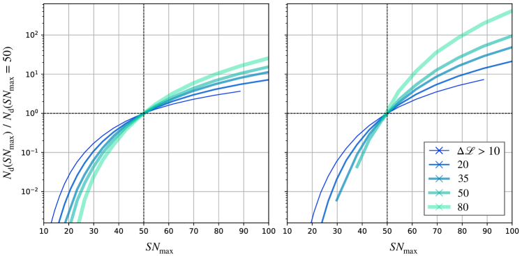
Fig. 7 shows the number of expected detections of haloes of mass, M⊙ (left panel) and M⊙ (right panel) for varying values of , normalized by the number of detections predicted for . The figure displays the case of our ‘quad’ configuration; results for our ‘arcs’ configuration are similar, albeit with a more marked dependence on the itself. Lines of different colour refer to different values of the log-likelihood threshold required for detectability. As expected, the number of detectable haloes is a rapidly increasing function of the signal-to-noise ratio. We find that, for a likelihood threshold of , an increase in signal-to-noise ratio from 50 to 60 corresponds to a doubling in the number of expected detections M. The same increase in data quality makes the expected detections M grow by a factor of three. As shown in the same figure, these factors are even larger if higher values of the log-likelihood ratio are required for detectability. For a value of , analogous to what has been used in most previous studies, we find the corresponding figures to be 2.5 and 5 for haloes of M⊙ and M⊙ respectively. It should be noted that an increase in the maximum ratio from 50 to 60 corresponds to an increase in the exposure time of a factor of , which is therefore smaller than the corresponding gain in the number of detectable haloes.

5.2 The effect of redshift dependence
We now examine the consequences of dropping the simplifying assumption of a tight relationship between halo mass and redshift. We isolate this effect by considering a population of CDM haloes assumed to lie on the Ludlow et al. (2016) mass-concentration relation, i.e. with reference to the previous Section, here we ignore the scatter in halo concentration. (We will consider this shortly.) Fig. 8 shows the redshift distribution of the population of detected haloes of mass, M⊙, we obtain when: for our two lensing configurations
- •
-
•
using the full redshift dependence of our log-likelihood maps, shown by a solid line.
As expected, the two curves match at , but we predict significantly fewer detections for foreground haloes, a reflection of the dependence on redshift of the log-likelihood increase described in Sect. 4.1. We also find that collapsing the redshift axis leads to an overestimate of detectable haloes also at , though by a smaller factor.
The magnitude of the global overestimate varies with the lensing configuration. For definitiveness, we use a threshold of in Fig. 8. For the arcs configuration, the overestimate is a factor 1.95; for the quad configuration it is a factor of 1.63. We stress that these figures should not be used to ‘correct’ previous measurements of the number of detectable haloes and are meant only as an estimate of the magnitude of the effect.


5.3 The effect of the scatter in concentration
We now consider the effect of accounting for scatter in the mass-concentration relation. We again focus on a population of CDM haloes, and compare the case in which all haloes are assumed to lie exactly on the median mass-concentration relation, to the case in which a lognormal scatter is included. For definitiveness, in both cases we use the full redshift dependence of the log-likelihood increase, , and, for simplicity, we restrict attention to our quad configuration. Results are analogous for our ‘arcs’ lensing morphology.
Fig. 9 shows the distribution of detectable haloes in the space of halo mass and shift relative to the median halo concentration, for the case in which the scatter in concentration is accounted for. The 2 dimensional histogram in the top panel is for an assumed threshold, . The vertical dashed line shows the median mass-concentration relation, . It is clear that, thanks to the dependence on concentration of the log-likelihood increase described in Section 4.2, most detectable haloes are high-concentration haloes. This is quantified in the bottom panel of the figure, which collapses the mass axis to show the distribution of detected haloes over concentration shifts. For reference, the dashed line shows the Gaussian distribution of all cosmological haloes. Coloured lines show the distribution of the population of detectable haloes for different values of the log-likelihood threshold, .
Haloes with high concentration achieve more easily, so that higher thresholds for detectability correspond to increasingly concentrated populations of detectable haloes. For and our quad configuration, we find when including all haloes of M⊙. The average concentration shift increases further for decreasing perturber masses, as shown by the coloured lines in the top panel. These represent the ‘mass-concentration relation of detectable haloes’. Lower mass haloes require stronger concentration boosts to achieve detectability, so that for , for haloes of M⊙.

The result is that the scatter in the mass-concentration relation boosts the number of expected detections. At low halo masses, for any fixed halo mass, there is a fraction of haloes with high enough concentration that become detectable if the scatter in the mass-concentration relation is accounted for, and which is lost when . This is quantified in Fig. 10, which shows the ratio between the cumulative number of detectable haloes, , predicted when accounting for the scatter in the mass-concentration relation, to the corresponding number obtained when for all haloes. Lines of different colours refer to different values of the detection threshold, . For all thresholds, the ratios are a strong function of halo mass. The onset of the sharp rise identifies the halo mass that is not detectable at that threshold if , but for which detections are possible because of concentration effects. For , even including all haloes with M⊙, concentration effects boost the number of detectable haloes by a factor of 2.75 for our ‘quad’ configuration. Since our ‘arcs’ configuration leads to lower values of the log-likelihood increase and fewer detections, the corresponding boost is a factor , exemplifying, on the one hand, the importance of concentration effects, and, on the other, the need for estimates tailored to the specific lensing configuration.
Fig. 11 displays the same boost factor as a function of the number of expected detections, (which include the effect of concentration). Different values of the expected number of detections correspond to different values of the data (or equivalently, different values of the log-likelihood threshold for detection). Once again we see that the exact figures depend on the lens configuration; for example, here the arcs configuration appears more sensitive to concentration effects than the quad.
5.4 The effect of concentration on distinguishing DM models
In most previous estimates of the dependence of the number of detectable haloes on the properties of the DM model, particularly the mass of a WDM particle (or, equivalently, the cutoff mass in the mass function) it was assumed that all haloes lie exactly on the median mass-concentration relation of CDM haloes. Not only is this a poor approximation but it left the differences in the halo abundances alone as the statistic to differentiate amongst different models. Our results show that concentration is a crucial ingredient for halo detectability. Warmer WDM models make low-mass haloes that are progressively less concentrated, as quantified by equation 21. This makes the concentration parameter potentially helpful in boosting the spread among the expected numbers of detections in different DM models.
We test this in Fig. 12, in which we show, side by side, the cumulative number of expected detections, , for a range of WDM models, parameterized by their cutoff mass, . The panel on the right displays results for the case in which concentration effects are neglected whereas the panel on the left includes both: (i) the scatter in the mass-concentration relation and (ii) the dependence of the median concentration on the DM model. For definitiveness, we show results pertaining to our ‘quad’ configuration, using a threshold for detection of .
It is clear that concentration effects significantly enhance the dependence of the expected number of detections on the DM model. Reduced concentration values act together with reduced cosmological abundances to determine the expected number of detections. Once again, while the qualitative trend is clear and the magnitude of the effect significant, precise values are dependent on the lensing configuration and on the value of the threshold chosen for detection. We attempt to quantify how much concentration effects can actually sharpen substructure lensing constraints in Section 6.1.
6 Discussion and Conclusions
We have quantified the ability of low-mass DM haloes along the line-of-sight to perturb strong gravitational lenses, and explored how this depends on halo properties. This is a fundamental ingredient of sensitivity mapping, that is the process of assessing which perturbers, out of the cosmological population of haloes, would actually be detectable when modelling strong lensing data. It is impossible to quantify the number of expected detections in different DM models in a given observational dataset without building the sensitivity function. Therefore, sensitivity mapping is a key aspect of placing constraints on the identity and properties of DM from the number of perturbing haloes detected in strong lensing studies.
We have adopted a likelihood-based approach, i.e. we differentiate between detectable and non-detectable haloes according to the likelihood gain, , associated with including a halo mass component in the lens modelling. Some previous studies have proposed using instead the Bayesian evidence for this comparison. It should be stressed that both approaches are equally valid. As long as the same criterion is consistently applied to both measure the sensitivity function — and therefore make predictions for the different DM models — and detect perturbers in the data, both approaches will return the correct inference on the DM properties if the models used in sensitivity mapping share the same complexities of the real data.
At this stage, it cannot be excluded that the sensitivity functions derived using likelihood or Bayesian evidence may exhibit some differences when compared side by side, possibly reflecting that the two criteria may lead to different sensitivity to perturbers in different regions of the parameter space. However, it seems quite unlikely that this would happen systematically at the high levels of significance that we are considering here and that have become the norm in structure lensing. At present, an evidence-based sensitivity function has not been derived as a function of either redshift or halo concentration, where our major findings are. Therefore, we are unable to make a direct comparison and have limited our analysis to the differences with the approximate strategies that have been adopted so far.
Rather than attempting to quantify the number of expected detections for specific observed strong lenses, we have focused on building an understanding of the sensitivity function itself, and how this scales with some of the crucial parameters at play. We have concentrated on the importance of image depth, and shown that, as the log-likelihood difference scales with , high signal-to-noise data are extremely beneficial in that they allow the detection of a larger number of perturbers, particularly of low-mass haloes (see Fig. 7). We have also shown that the specific noise realization introduces scatter in the log-likelihood difference, of magnitude (see Sect. 3.2), which suggests that a smooth link between the probability of detection, , and the log-likelihood gain, rather than a sharp threshold, may be a better choice when comparing with real data.
We find that our two different lens configurations yield significantly different numbers of expected halo detections, which indicates that some lensing morphologies (a quad configuration in our case) are more valuable for strong lensing analyses (see Fig. 6). This will be useful in selecting lenses to target with deeper observations. We also note that our estimates for the total number of detectable haloes are somewhat lower than what has been suggested by similar studies for the same values of lens and source redshifts, and for similar data quality. This may be due to the increased flexibility of our lens modelling, including the possibility of shifts in the lens centre (see Vegetti et al., 2014), as well as the assumed power-law profile slope (see Li et al., 2017; Despali et al., 2018). With particular reference to Li et al. (2017) and Despali et al. (2018), the fact that we perform fully non-linear searches when optimising our macromodels certainly enables them to reproduce better the perturbed data without the need of including a halo mass component, hence lowering the log-likelihood gain. If anything, this highlights the importance of using exactly the same techniques to both i) model real data and make perturber detections and ii) produce estimates of the expected detections, as any mismatch would inevitably introduce systematic biases.
We then concentrated on the role of halo redshift and halo concentration. In previous work, simplifications had been made to collapse these axes, in order to make the calculation of the sensitivity function computationally feasible.
Concerning the redshift of the perturber, we have shown that, contrary to previous understanding, it becomes increasingly challenging to detect perturbing haloes in front of the main lens when they get closer to the observer (see Figs. 2, 3 and 4). This implies that previous studies of the number of detectable haloes have likely overestimated the number of foreground detections, at redshifts . The exact magnitude of this overestimation appears to depend on the specific lensing configuration. As a reference, our experiments show this factor to be between 1.5 and 2 (see Fig. 8). These previous estimates are not based on a calculation of the Bayesian evidence at . Therefore, it is not currently known whether an evidence-based criterion for detection would indeed yield a dependence of the perturbers’ detectability on redshift that is analogous to the one we measure. Certainly, we find that the strategy adopted so far (of using deflection angles as proxies) underestimates the degree of degeneracy in the lens modelling and therefore artificially makes the detection of foreground perturbers easier than in actually is in reality.
Concerning concentration, we find that detectability is a strong function of halo concentration, such that the population of detectable haloes is, in fact, a population of systematically high-concentration haloes (see Fig. 9). The shift in the average concentration relative to the mass-concentration relation becomes increasingly large for haloes of lower masses, and increases when a higher threshold for detectability is adopted. For a threshold of , the average shift in the concentration of haloes with masses below M⊙ is about , where is the lognormal scatter in the mass-concentration relation.
Crucially, accounting for the scatter in the mass-concentration relation results in a boost to the number of detectable haloes. This boost is a strong function of the lensing configuration and of the threshold for detectability (or, equivalently, of the data quality as quantified by the maximum signal-to-noise; see Figs. 10 and 11). As reference, for a combination of a lens configuration and detection threshold that results in a total of 0.03 detections with M⊙ per lens in a CDM universe – which is roughly comparable to what was previously predicted for lenses with HST data – this boost amounts to a factor of , and quickly grows to for the detections expected at M⊙.
Unfortunately, without a tailored study, it is impossible to provide a precise quantification of how the two effects above would combine to affect previous estimates of the expected number of detections in real observed strong lenses, especially since the two effects have opposite signs. The overestimate related to the redshift dependence is sensitive to the lensing configuration and, certainly to the redshifts of both lens and source, which here we have kept fixed. The underestimate due to the concentration dependence is a strong function of lensing configuration and data quality. It would appear that the correction due to concentration is larger than that due to the redshift dependence, but further study is required to ascertain in which regime that is the case, and by how much.
What we can already establish in the present study is how concentration effects can facilitate differentiating WDM models with different cutoff halo masses. We have shown that taking into account the dependence of the median halo concentration on the DM model increases the spread among the number of expected detections (see Fig. 12). For warmer models, lower halo concentrations conspire with lower cosmological halo abundances increasingly to suppress the number of detectable haloes. The effect of halo concentration had not been included in previous studies, leaving only halo abundances to differentiate among DM models, therefore making it harder to distinguish them in strong lensing studies.

6.1 Sharper DM constraints from substructure lensing
In order to quantify the extent to which concentration effects can sharpen future substructure lensing constraints, we assume we have a set of strong lenses such that the total expected number of detections in CDM is
| (23) |
We ignore the contribution of satellite haloes, and assume that the figure above only includes haloes along the LOS, on which we have focussed in this work. While we are not able to tailor our analysis quantitatively to any specific set of observed strong lenses, this figure is representative of what is achievable with current HST data (Vegetti et al., 2018; Ritondale et al., 2019), and therefore provides a useful reference point. We use our maps of log-likelihood increase, , to calculate the number of expected detections in the same set of lenses for WDM models with different cutoff masses, . We do so separately for our ‘quad’ and ‘arcs’ lensing configurations, requiring that the number of lenses in the two separate sets be such as to satisfy Equation 23 separately777 We require a detection threshold, , for our quad configuration and for our arcs configuration, which, as we have shown, leads to systematically fewer detections per lens.. Furthermore, we set up predictions for both, the case in which concentration effects are accounted for and the case in which they are ignored. Then, we compare the inferences on the DM model that would result from actually detecting individual haloes, in the two different configurations. These are displayed in Fig. 13, which shows the likelihood ratio,
| (24) |
where is the Poisson probability distribution with mean, , and is the number of actual detections. Inference resulting from predictions that ignore concentration effects are shown with dashed lines, while the likelihood ratio obtained when accounting for concentration effects is shown with solid lines. The vertical lines indicate the limits on the WDM cutoff mass corresponding to a likelihood ratio of . The right and left columns correspond, respectively, to the two lensing configurations. Details are only marginally different and the magnitude of the effect is very similar in the two cases: at fixed number of expected haloes in a CDM universe, concentration effects make constraints on the WDM cutoff mass significantly more stringent. The suppression in the concentration of WDM haloes enhances the effect of lower cosmological halo abundances, allowing constraints that are about one order of magnitude more stringent in .
6.2 Outlook
Our results bring renewed confidence to the field of halo detection with strong lensing data, and boost confidence that meaningful constraints can be obtained from analysis of current optical data. A number of previous works have contributed to the realization that it is extremely challenging to use current optical HST data to obtain constraints on the cutoff of the DM halo mass function that are competitive with those obtained from the satellites of the Milky Way or measurements of the Lyman- forest (see Enzi et al., 2021, and references therein). This is because, if halo abundances alone are used to differentiate between CDM and WDM, in order to be able to probe a WDM model with a cutoff mass, (the mass below which the abundance of haloes declines sharply), it is necessary to be sensitive to perturbers of that halo mass and below. However, evidence is mounting that detecting haloes of mass M⊙ is extremely challenging with current lensing data, and therefore that it would be very difficult to place competitive constraints.
Concentration effects change this picture completely. For example, the limits displayed in Fig. 13 stem from detections of haloes of mass M⊙ – which is realistic with current HST data – but they can rule out values of the cutoff mass scale, M⊙. This is a direct reflection of the effects of halo concentration, which, in contrast to halo abundances, first affects haloes of masses significantly above the cutoff mass itself. For this reason, concentration effects allow substructure lensing studies to probe WDM models with cutoff masses at least one order of magnitude below the lowest sensitivity mass scale. This implies that substructure lensing is, in fact, a much more sensitive probe of the identity of the DM than had been previously recognized.
Software Citations
This work used the following software packages:
- •
- •
-
•
matplotlib (Hunter et al., 2007)
- •
-
•
PyAutoLens (Nightingale & Dye, 2015; Nightingale, Dye, & Massey, 2018; Nightingale et al., 2021)
- •
- •
Acknowledgements
NCA is supported by an STFC/UKRI Ernest Rutherford Fellowship, Project Reference: ST/S004998/1. JWN and RJM acknowledge funding from the UKSA through awards ST/V001582/1 and ST/T002565/1; RJM is also supported by the Royal Society. ARR is supported by the European Research Council Horizon2020 grant ‘EWC’ (award AMD-776247-6). CSF acknowledges support by the European Research Council (ERC) through Advanced Investigator grant to CSF, DMIDAS (GA 786910). RL acknowledge the support of National Nature Science Foundation of China (Nos 11773032,12022306). This work used the DiRAC Data Centric system at Durham University, operated by the Institute for Computational Cosmology on behalf of the STFC DiRAC HPC Facility (www.dirac.ac.uk). This equipment was funded by BIS National E-infrastructure capital grant ST/K00042X/1, STFC capital grants ST/H008519/1 and ST/K00087X/1, STFC DiRAC Operations grant ST/K003267/1 and Durham University. DiRAC is part of the National E-Infrastructure.
Appendix A Input macromodels
Table 1 contains values of the adopted model parameters for the two different lensing configurations used in this study.
| Model parameter | quad | arcs |
|---|---|---|
| (0.0051”, 0.0765”) | (0.0396”, 0.08”) | |
| 1.165” | 1.095” | |
| 1.93 | 1.99 | |
| (0.022, 0.011) | (-0.013, 0.007) | |
| (-0.037, -0.099) | (-0.008, 0.001) | |
| 0.5 | 0.5 | |
| (0.024”, 0.032”) | (-0.024, 0.036) | |
| 0.15” | 0.12” | |
| (0.147, -0.135) | (0.05, -0.25) | |
| 1.1 | 1.2 | |
| 1 | 1 | |
| 1.0 | 1.0 |
Appendix B Dependence on the noise realization
Fig. 14 shows the link between the mean and the scatter (standard deviation) of the log-likelihood gain . Each point corresponds to a different set of halo properties . For each, 10 different random noise realizations have been considered and modelled. The corresponding set of values for the log-likelihood increase has been used to estimate both mean value and standard deviation. The red dashed line illustrates the prediction of equation (15).

References
- Alam et al. (2017) Alam S., Ata M., Bailey S., Beutler F., Bizyaev D., Blazek J. A., Bolton A. S., et al., 2017, MNRAS, 470, 2617. doi:10.1093/mnras/stx721
- Angulo et al. (2012) Angulo R. E., Springel V., White S. D. M., Jenkins A., Baugh C. M., Frenk C. S., 2012, MNRAS, 426, 2046. doi:10.1111/j.1365-2966.2012.21830.x
- Astropy Collaboration (2013) Astropy Collaboration, 2013, aap, 558, A33. doi:10.1051/0004-6361/201322068
- Avila-Reese et al. (2003) Avila-Reese V., Colín P., Piccinelli G., Firmani C., 2003, ApJ, 598, 36. doi:10.1086/378773
- Baur et al. (2016) Baur J., Palanque-Delabrouille N., Yèche C., Magneville C., Viel M., 2016, JCAP, 2016, 012. doi:10.1088/1475-7516/2016/08/012
- Benedikt et al. (2018) Benedikt D., 2018, Astrophys. J., Suppl. Ser., 2, 35. doi:10.3847/1538-4365/aaee8c
- Benitez-Llambay & Frenk (2020) Benitez-Llambay, A. & Frenk, C. 2020, MNRAS, 498, 4887. doi:10.1093/mnras/staa2698
- Birrer, Amara, & Refregier (2016) Birrer S., Amara A., Refregier A., 2016, JCAP, 2016, 020. doi:10.1088/1475-7516/2016/08/020
- Bolton (2005) Bolton A. S., 2005, PhDT
- Bose et al. (2016) Bose S., Hellwing W. A., Frenk C. S., Jenkins A., Lovell M. R., Helly J. C., Li B., 2016, MNRAS, 455, 318. doi:10.1093/mnras/stv2294
- Boyarsky et al. (2019) Boyarsky A., Drewes M., Lasserre T., Mertens S., Ruchayskiy O., 2019, PrPNP, 104, 1. doi:10.1016/j.ppnp.2018.07.004
- Davis et al. (1985) Davis M., Efstathiou G., Frenk C. S., White S. D. M., 1985, ApJ, 292, 371. doi:10.1086/163168
- Despali et al. (2018) Despali G., Vegetti S., White S. D. M., Giocoli C., van den Bosch F. C., 2018, MNRAS, 475, 5424. doi:10.1093/mnras/sty159
- Despali et al. (2020) Despali G., Lovell M., Vegetti S., Crain R. A., Oppenheimer B. D., 2020, MNRAS, 491, 1295. doi:10.1093/mnras/stz3068
- Diemand et al. (2008) Diemand J., Kuhlen M., Madau P., Zemp M., Moore B., Potter D., Stadel J., 2008, Natur, 454, 735. doi:10.1038/nature07153
- Dye & Warren (2005) Dye S., Warren S. J., 2005, ApJ, 623, 31. doi:10.1086/428340
- Enzi et al. (2021) Enzi, W., Murgia, R., Newton, O., et al. 2021, MNRAS, 506, 5848. doi:10.1093/mnras/stab1960
- Frenk & White (2012) Frenk C. S., White S. D. M., 2012, AnP, 524, 507. doi:10.1002/andp.201200212
- Garzilli, Boyarsky, & Ruchayskiy (2017) Garzilli A., Boyarsky A., Ruchayskiy O., 2017, PhLB, 773, 258. doi:10.1016/j.physletb.2017.08.022
- Garzilli et al. (2019) Garzilli A., Ruchayskiy O., Magalich A., Boyarsky A., 2019, arXiv, arXiv:1912.09397
- Gilman et al. (2020) Gilman D., Du X., Benson A., Birrer S., Nierenberg A., Treu T., 2020, MNRAS, 492, L12. doi:10.1093/mnrasl/slz173
- Gilman et al. (2019) Gilman D., Birrer S., Treu T., Nierenberg A., Benson A., 2019, MNRAS, 487, 5721. doi:10.1093/mnras/stz1593
- Gilman et al. (2018) Gilman D., Birrer S., Treu T., Keeton C. R., Nierenberg A., 2018, MNRAS, 481, 819. doi:10.1093/mnras/sty2261
- Green, Hofmann, & Schwarz (2005) Green A. M., Hofmann S., Schwarz D. J., 2005, JCAP, 2005, 003. doi:10.1088/1475-7516/2005/08/003
- Harvey et al. (2020) Harvey D., Valkenburg W., Tamone A., Boyarsky A., Courbin F., Lovell M., 2020, MNRAS, 491, 4247. doi:10.1093/mnras/stz3305
- Hastie, Tibshirani, & Friedman (2008) Hastie T., Tibshirani R., Friedman J., 2008, The Elements of Statistical Learning, Springer New York Inc.
- Hezaveh et al. (2016) Hezaveh Y. D., Dalal N., Marrone D. P., Mao Y.-Y., Morningstar W., Wen D., Blandford R. D., et al., 2016, ApJ, 823, 37. doi:10.3847/0004-637X/823/1/37
- Hunter et al. (2007) Hunter, J. D., 2007, aj, 9, 3. doi:10.1109/MCSE.2007.55
- Iršič et al. (2017) Iršič V., Viel M., Haehnelt M. G., Bolton J. S., Cristiani S., Becker G. D., D’Odorico V., et al., 2017, PhRvD, 96, 023522. doi:10.1103/PhysRevD.96.023522
- Jenkins et al. (2001) Jenkins A., Frenk C. S., White S. D. M., Colberg J. M., Cole S., Evrard A. E., Couchman H. M. P., et al., 2001, MNRAS, 321, 372. doi:10.1046/j.1365-8711.2001.04029.x
- Kennedy et al. (2014) Kennedy, R., Frenk, C., Cole, S., et al. 2014, MNRAS, 442, 2487. doi:10.1093/mnras/stu719
- Konishi & Kitagawa (2007) Konishi S., Kitagawa G., 2007, Information Criteria and Statistical Modeling, Springer New York Inc.
- Li et al. (2017) Li R., Frenk C. S., Cole S., Wang Q., Gao L., 2017, MNRAS, 468, 1426. doi:10.1093/mnras/stx554
- Lovell et al. (2012) Lovell M. R., Eke V., Frenk C. S., Gao L., Jenkins A., Theuns T., Wang J., et al., 2012, MNRAS, 420, 2318. doi:10.1111/j.1365-2966.2011.20200.x
- Lovell et al. (2014) Lovell M. R., Frenk C. S., Eke V. R., Jenkins A., Gao L., Theuns T., 2014, MNRAS, 439, 300. doi:10.1093/mnras/stt2431
- Lovell et al. (2016) Lovell, M. R., Bose, S., Boyarsky, A., et al. 2016, MNRAS, 461, 60. doi:10.1093/mnras/stw1317
- Ludlow et al. (2016) Ludlow A. D., Bose S., Angulo R. E., Wang L., Hellwing W. A., Navarro J. F., Cole S., et al., 2016, MNRAS, 460, 1214. doi:10.1093/mnras/stw1046
- Minor et al. (2021) Minor Q., Kaplinghat M., Chan T. H., Simon E., 2021, MNRAS.tmp. doi:10.1093/mnras/stab2209
- Navarro, Frenk, & White (1997) Navarro J. F., Frenk C. S., White S. D. M., 1997, ApJ, 490, 493. doi:10.1086/304888
- Neto et al. (2007) Neto, A. F., Gao, L., Bett, P., et al. 2007, MNRAS, 381, 1450. doi:10.1111/j.1365-2966.2007.12381.x
- Newton et al. (2020) Newton, O., Leo, M., Cautun, M., et al. 2020, arXiv:2011.08865
- Nightingale & Dye (2015) Nightingale J. W., Dye S., 2015, MNRAS, 452, 2940. doi:10.1093/mnras/stv1455
- Nightingale, Dye, & Massey (2018) Nightingale J. W., Dye S., Massey R. J., 2018, MNRAS, 478, 4738. doi:10.1093/mnras/sty1264
- Nightingale et al. (2019) Nightingale J. W., Massey R. J., Harvey D. R., Cooper A. P., Etherington A., Tam S.-I., Hayes R. G., 2019, MNRAS, 489, 2049. doi:10.1093/mnras/stz2220
- Nightingale et al. (2021) Nightingale J. W., Hayes R. G., Kelly A., Amvrosiadis A., Etherington A., He Q., Li N., et al., 2021, JOSS, 6, 58, doi:10.21105/joss.02825
- Planck Collaboration et al. (2020) Planck Collaboration, Aghanim N., Akrami Y., Ashdown M., Aumont J., Baccigalupi C., Ballardini M., et al., 2020, A&A, 641, A6. doi:10.1051/0004-6361/201833910
- Powell et al. (2021) Powell D., Vegetti S., McKean J. P., Spingola C., Rizzo F., Stacey H. R., 2021, MNRAS, 501, 515. doi:10.1093/mnras/staa2740
- Price-Whelan et al. (2018) Price-Whelan A.M., Sipocz B.M., Gunther H.M., Lim P.L., Crawford S.M., et al., 2018, aj, 156, 123. doi:10.3847/1538-3881/aabc4f
- Richings et al. (2021) Richings J., Frenk C., Jenkins A., Robertson A., Schaller M., 2021, MNRAS, 501, 4657. doi:10.1093/mnras/staa4013
- Ritondale et al. (2019) Ritondale E., Vegetti S., Despali G., Auger M. W., Koopmans L. V. E., McKean J. P., 2019, MNRAS, 485, 2179. doi:10.1093/mnras/stz464
- Schneider et al. (2012) Schneider A., Smith R. E., Macciò A. V., Moore B., 2012, MNRAS, 424, 684. doi:10.1111/j.1365-2966.2012.21252.x
- Sheth, Mo, & Tormen (2001) Sheth R. K., Mo H. J., Tormen G., 2001, MNRAS, 323, 1. doi:10.1046/j.1365-8711.2001.04006.x
- Shu et al. (2016) Shu Y., Bolton A. S., Kochanek C. S., Oguri M., Pérez-Fournon I., Zheng Z., Mao S., et al., 2016, ApJ, 824, 86. doi:10.3847/0004-637X/824/2/86
- Springel et al. (2005) Springel V., White S. D. M., Jenkins A., Frenk C. S., Yoshida N., Gao L., Navarro J., et al., 2005, Natur, 435, 629. doi:10.1038/nature03597
- Suyu et al. (2006) Suyu S. H., Marshall P. J., Hobson M. P., Blandford R. D., 2006, MNRAS, 371, 983. doi:10.1111/j.1365-2966.2006.10733.x
- Tessore et al. (2016) Tessore N., Bellagamba F., Metcalf B., 2016, MNRAS, 463, 3115. doi:10.1093/mnras/stw2212
- van der Walt et al. (2011) van der Walt S., Colbert S. C., Varoquaux G., 2011, Computing in Science Engineering, 13, 2. doi:10.1109/MCSE.2011.37
- Van Rossum et al. (2009) Van Rossum G., Drake F. L., 2009, Python 3 Reference Manual, isbn:1441412697
- Vegetti & Koopmans (2009) Vegetti S., Koopmans L. V. E., 2009, MNRAS, 392, 945. doi:10.1111/j.1365-2966.2008.14005.x
- Vegetti et al. (2010) Vegetti S., Koopmans L. V. E., Bolton A., Treu T., Gavazzi R., 2010, MNRAS, 408, 1969. doi:10.1111/j.1365-2966.2010.16865.x
- Vegetti et al. (2012) Vegetti S., Lagattuta D. J., McKean J. P., Auger M. W., Fassnacht C. D., Koopmans L. V. E., 2012, Natur, 481, 341. doi:10.1038/nature10669
- Vegetti et al. (2014) Vegetti S., Koopmans L. V. E., Auger M. W., Treu T., Bolton A. S., 2014, MNRAS, 442, 2017. doi:10.1093/mnras/stu943
- Vegetti et al. (2018) Vegetti S., Despali G., Lovell M. R., Enzi W., 2018, MNRAS, 481, 3661. doi:10.1093/mnras/sty2393
- Viel et al. (2013) Viel M., Becker G. D., Bolton J. S., Haehnelt M. G., 2013, PhRvD, 88, 043502. doi:10.1103/PhysRevD.88.043502
- Virtanen et al. (2020) Virtanen P., Gommers R., Oliphant Travis E., Haberland M., Reddy M., et al., 2011, Nature Methods, 17, 261-272 doi:10.1038/s41592-019-0686-2
- Wang et al. (2016) Wang W., White S. D. M., Mandelbaum R., Henriques B., Anderson M. E., Han J., 2016, MNRAS, 456, 2301. doi:10.1093/mnras/stv2809
- Wang et al. (2020) Wang J., Bose S., Frenk C. S., Gao L., Jenkins A., Springel V., White S. D. M., 2020, Natur, 585, 39. doi:10.1038/s41586-020-2642-9
- Warren & Dye (2003) Warren S. J., Dye S., 2003, ApJ, 590, 673. doi:10.1086/375132
- Xu et al. (2015) Xu D., Sluse D., Gao L., Wang J., Frenk C., Mao S., Schneider P., et al., 2015, MNRAS, 447, 3189. doi:10.1093/mnras/stu2673