Gyrokinetic simulations in stellarators using different computational domains
Abstract
In this work, we compare gyrokinetic simulations in stellarators using different computational domains, namely, flux tube, full-flux-surface, and radially global domains. Two problems are studied: the linear relaxation of zonal flows and the linear stability of ion temperature gradient (ITG) modes. Simulations are carried out with the codes EUTERPE, GENE, GENE-3D, and stella in magnetic configurations of LHD and W7-X using adiabatic electrons. The zonal flow relaxation properties obtained in different flux tubes are found to differ with each other and with the radially global result, except for sufficiently long flux tubes, in general. The flux tube length required for convergence is configuration-dependent. Similarly, for ITG instabilities, different flux tubes provide different results, but the discrepancy between them diminishes with increasing flux tube length. Full-flux-surface and flux tube simulations show good agreement in the calculation of the growth rate and frequency of the most unstable modes in LHD, while for W7-X differences in the growth rates are found between the flux tube and the full-flux-surface domains. Radially global simulations provide results close to the full-flux-surface ones. The radial scale of unstable ITG modes is studied in global and flux tube simulations finding that in W7-X, the radial scale of the most unstable modes depends on the binormal wavenumber, while in LHD no clear dependency is found.
Keywords: stellarator, gyrokinetic simulations, flux tube, full surface, global, ITG, zonal flows
1 INTRODUCTION
Gyrokinetics is the theoretical framework to study microturbulence in magnetized plasmas. It takes advantage of scale separation between turbulent fluctuations and background quantities (such as magnetic geometry and plasma profiles), and provides a reduction of phase-space dimensionality, which allows an important saving of computational resources. In tokamaks, the theoretical analysis and the numerical simulation of microinstabilities and turbulence are largely facilitated by its axisymmetry, which makes all the field lines on a flux surface equivalent, so that simulations can be carried out in a reduced spatial domain called flux tube (FT): a volume extending several Larmor radii around a magnetic field line. Thanks to axisymmetry, the result of a calculation in a flux tube is independent of the chosen magnetic field line. Periodic boundary conditions in the parallel direction and the standard twist-and-shift formulation [1] are commonly used.
The lack of axisymmetry in stellarators introduces complexity at several levels. First, the twist-and-shift boundary condition in flux tube simulations is questionable [2] due to the three-dimensional dependence of the equilibrium quantities affecting micro-instabilities, such as magnetic field line curvature and magnetic shear. As a consequence of this dependence, different flux tubes over a given flux surface are in general not equivalent to each other [3]. A common practice when using flux tube codes in stellarators is to simulate the most unstable flux tube, which allows to quantify the upper bound of the instability. However, the turbulence saturation level can be largely affected by the interaction between small-scale fluctuations and zonal flows (ZF), and the long time behaviour of the latter (which, in stellarators, shows distinct features as compared to tokamaks [4, 5, 18]) depends on the magnetic geometry of the whole flux surface. Different saturation mechanisms can dominate in different devices depending on the magnetic geometry [7]. In addition, the radial electric field, whose effect cannot be accounted for in a flux tube domain, might play a role in the linear stability [8, 9] and the turbulence saturation.
In this work, we address the question of which is the minimum computational domain appropriate for the simulation of instabilities and zonal flows in stellarators and we study to what extent simplified setups, such as the flux tube approximation, can be used. For this purpose, we compare gyrokinetic simulations in different stellarator configurations using different computational domains and codes. The codes used are EUTERPE [10], GENE [12], GENE-3D [13] (the radially global version of GENE for stellarators), and stella [11], which cover different computational domains and implement different numerical methods. stella is a flux tube continuum code. Both a flux tube and a full-flux-surface version of GENE are available for stellarators. EUTERPE and GENE-3D are both radially global, although with different numerical schemes; EUTERPE is a particle-in-cell (PIC) code while GENE-3D is a continuum code.
Two problems are studied with these codes: the linear relaxation of zonal flows and the linear stability of Ion Temperature Gradient (ITG) modes. The first one has been studied both analytically and numerically in helical [14, 15, 16] and general stellarator geometries [17, 4, 5, 6, 18], showing distinct features as compared to tokamaks. The (semi)analytical calculations were validated against numerical simulations with EUTERPE, in the radially global (RG) domain, and GENE, in the full-flux-surface (FFS) domain, in W7-X and LHD configurations, finding a remarkable agreement [6, 18]. The linear relaxation of zonal flows in FT, FFS, and RG domains has been compared in HSX and NCSX configurations [19]. In this work, we provide additional comparisons for LHD and W7-X in order to complete the picture of how the computational domain choice impacts the linear ZF relaxation. We study this problem in the flux tube domain, and compare the results with those obtained in the FFS and RG domains, which was not previously done in these configurations. With respect to the ITG linear stability, no systematic comparison between different computational domains has been reported so far for stellarators. In this contribution, we compare results from ITG simulations carried out in FT, FFS and RG domains in the same configurations. Good convergence between different FT results is found in LHD, while in W7-X significant differences are found between calculations in different flux tubes.
The rest of the paper is organized as follows. In section 2, the computational domains and the codes used in this work are introduced. For LHD and W7-X and the computational domains considered, the collisionless linear ZF relaxation is studied in section 3, while the linear stability of the Ion Temperature Gradient (ITG) mode is presented in section 4. Finally, in section 5 the results are discussed and some conclusions are drawn.
2 Computational domains and codes
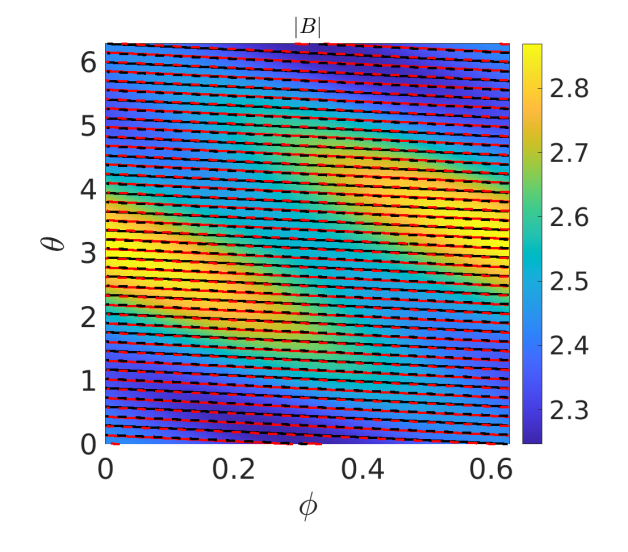
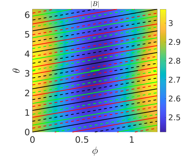
We devote this section to describing the different computational domains and codes used in this work, and start describing the simplest computational domain, the flux tube. A flux tube domain is defined by a volume around a magnetic field line, which extends a finite length along the direction parallel to the magnetic field. We will refer generically to spatial coordinates that will be defined for each code later on, with a coordinate in the radial direction, a coordinate along the magnetic field line and a coordinate in the binormal direction, i.e. perpendicular to both the magnetic field and the flux surface normal vector. Twist and shift boundary conditions are defined in the direction parallel to the magnetic field [1]. The length of the flux tube is usually measured in terms of poloidal turns, . In a tokamak, the axisymmetry makes that a flux tube that extends one poloidal turn samples completely the geometry of a flux surface. In stellarators, this is not the case due to the three dimensional dependence of the magnetic geometry. Flux tube simulations are local, i.e the width of the flux tube along the radial and binormal direction is sufficiently thin so that the turbulence can be assumed to depend only on the local values of the relevant quantities of the problem (density, temperature, geometric coefficients, etc.) at the radial and binormal location of the selected line. Periodic conditions in the radial direction are assumed. Only one radial mode and a perpendicular mode are scanned at a time in linear simulations. We consider two different flux tubes in this work: one centered with respect to the position and the other one centered with respect to the point , with N the periodicity of the device (N=5 for W7-X and N=10 for LHD) and and the angular PEST coordinates [20]. Each of these flux tubes will eventually cover different lengths, which will be expressed in terms of the number of poloidal turns. Figures 1 and 2 show, for the mid plasma radius, the magnetic field strength in a period of LHD (top) and W7-X (bottom) as well as the flux tubes considered for different number of poloidal turns. In Figure 3, several quantities related with the magnetic geometry that affect the linear zonal flow relaxation [18, 21] and ITG instability are represented along these two FTs and for the same magnetic configurations. Both FTs are stellarator symmetric, which means that the magnetic field is the same at both ends of the FT. A number of parallel wavenumbers depending on the spatial discretization along the field line is considered in the simulation. In nonlinear simulations, a box in the radial and binormal directions is defined around the central field line defining the FT, and a set of radial and binormal wavenumbers and are considered. The fulfilment of the periodicity condition in the parallel direction for all the modes considered in the simulation is more restrictive in this case, with a strong influence of the magnetic shear [1, 2, 22].


The full-flux-surface computational domain is defined by a region around a specific magnetic flux surface, at a fixed value of the radial coordinate. In this computational domain the locality along the binormal direction, which the FT approach assumes, is relaxed, while the domain is still local in the radial direction. This means that only the local values of magnetic field and profiles at the radial location at which the domain is centered are used in all the extent of the domain, and periodicity conditions are used in the radial direction. Multiple and modes are considered in either a linear or nonlinear simulation. Just a period of the device is simulated, usually, which means that modes that are not multiple of the device periodicity (N) are not considered in these simulations. In linear simulations either only one radial scale or a set of can be studied at a time. In nonlinear simulations a box in the radial direction is defined around the flux surface and a range of radial wavenumbers is considered. Similar to the FT case, some constraints are derived from setting periodicity conditions for all the considered.
The most complete computational domain is the radially global one. This domain consist of a volume covering the full flux surface and with a finite radial extent without assuming periodicity in the radial coordinate. The number of modes considered in a simulation using this domain depends on the spatial grids used in the angular directions along the flux surfaces and the radial direction. As in the FFS domain, usually just a period of the device is simulated and the same limitations in respect to the toroidal Fourier modes apply to this case. The domain can cover either the full radius or an annular region with inner and outer boundaries different from the magnetic axis and the last closed flux surface. In this work we will refer to both kinds of simulations as radially global. What distinguishes this domain from the FFS one is that in this case the values of magnetic field, the density and temperature profiles and their gradients are used at each specific position in the full 3D domain covered by the simulation. The effects of global radial profiles, or large scale radial structures are captured in this domain, while they are not in the FFS one. Multiple modes in the radial direction are considered in this kind of simulation either linear or nonlinear, which are determined by the radial discretization. The boundary conditions used at the inner and outer boundaries of the domain are usually not fully realistic and can affect the simulation in a special way. It is common practice defining, either explicitly or implicitly, a buffer region close to each boundary in which the potential is assumed to be affected not only by physical aspects but also by the boundary conditions. The central radial region located far from the boundaries is considered not to be significantly affected by the boundary treatment.
A radial electric field does not influence the result of flux tube simulations beyond a Doppler shift on the frequencies of the modes, while in FFS and RG domains, physical effects can be observed. The shearing effects of an electric field having a radial gradient cannot be easily accounted for in a FFS simulation domain while they are naturally included in a RG domain.
The codes used for the simulations in this work are all based on the gyrokinetic formalism and solve the Vlasov-Poisson equations using the approach, but they differ in several aspects of the numerical implementation.
EUTERPE is a particle-in-cell gyrokinetic code that can simulate the entire confined plasma or a volume covering a radial annulus [10, 23]. For the field solver, natural boundary conditions are set at the inner boundary for the full volume simulations, while Dirichlet conditions are used if the simulation is considering an annulus. Dirichlet conditions are always used at the outer boundary. Density and temperature profiles, depending only on the radial coordinate, are used as input for both kinds of simulations. PEST () magnetic coordinates [20] are used for the description of the fields, with , the toroidal flux, the toroidal flux at the last close flux surface, the toroidal angle, and the poloidal angle. The electrostatic potential is Fourier transformed on each flux surface considering a Fourier filter over a range of poloidal and toroidal mode numbers. EUTERPE features the possibility of extracting a phase factor in linear simulations, thus allowing for a significant reduction in the computational resources [10]. This feature takes advantage of the translation property of the Fourier transform to center the Fourier filter on the region of interest in the wavenumber space and is used for the exploration of the wavenumber spectrum of unstable ITG modes in a wide range (see section 4). Even using these tools, the computational resources required for these simulations are significantly larger than for FT simulations. For details about the code EUTERPE, the reader is referred to [10, 23, 24].
The current version of the stella code [11] solves, in the flux tube approximation, the gyrokinetic Vlasov and Poisson equations for an arbitrary number of species. The magnetic geometry can be specified either by the set of Miller’s parameters for a local tokamak equilibrium or by a three-dimensional equilibrium generated with VMEC [25]. The spatial coordinates that the code uses for stellarator simulations are: the flux surface label , with the minor radius; the magnetic field line label , with the Clebsch angle , the rotational transform and the radial location of the magnetic field lines surrounded by the simulated flux tube; and the parallel coordinate. The velocity coordinates are the magnetic moment and the parallel velocity . A mixed implicit-explicit integration scheme, which can be varied from fully explicit to partial or fully implicit, is used in this code. The implicit scheme has the advantage of allowing a larger time step than fully explicit approaches when considering kinetic electrons [11].
GENE is an Eulerian gyrokinetic code [12]. It uses a fixed grid in five-dimensional phase space (plus time), consisting of two velocity coordinates (velocity parallel to the magnetic field) and (magnetic moment), and the three magnetic field-aligned coordinates , with the radial coordinate, defined as , the coordinate along the binormal direction and the coordinate along the field line. For stellarator simulations, GENE can simulate either a flux tube or a full flux surface. In the former option, it is spectral in the coordinates perpendicular to the magnetic field , while in the later it uses a representation in real space for the binormal coordinate and a Fourier representation for the radial coordinate. In both cases, periodic boundary conditions are used in the perpendicular directions.
GENE-3D is a global gyrokinetic code for stellarators [13]. It solves the gyrokinetic equation in the same dimensional space as GENE. However, it uses a real representation of the spatial coordinates. GENE-3D can be used in either FT, FFS or RG domains. Periodic radial conditions are used when FT or FFS are simulated. In the RG case, Dirichlet boundary conditions are used at both the inner and outer radial boundaries.
In stella, GENE and GENE-3D it is common practice using hyperdiffusion terms, which allow the stabilization of sub-grid modes. While these terms are required for nonlinear simulations they can have a damping effect over the zonal components of the potential. In simulations devoted to study the linear relaxation of ZFs, like those presented in section 3, the hyperdiffusion has to be reduced significantly to avoid this damping, or alternatively, the resolution in velocity space has to be increased [26].
For all the codes, the equilibrium magnetic field is obtained from a magneto-hydrodynamic equilibrium calculation with the code VMEC, and selected magnetic quantities are mapped for its use in the gyrokinetic codes with the intermediate programs VM2MAG, GIST and GVEC for EUTERPE, GENE and GENE-3D, respectively. Note that in stella, GENE and GENE-3D the resolution used in the equilibrium magnetic field is coupled to the resolution in the electrostatic potential, while in EUTERPE, both resolutions are independent.
In the simulations presented in this work, the same density and temperature profiles are used in the global codes, using the local values of , , , and their scale lengths , , and (with ) at the reference position, , in the radially local codes, with . The simulations presented here are all electrostatic and use adiabatic electrons.
3 Linear relaxation of zonal flows
| LHD | code | domain | markers | hyp’z | hyp’v | |||||||
| GENE | FT | 1 | 1 | 144 | 28 | 0.1 | 0.1 | |||||
| FFS | 1 | 1 | 144 | 28 | 0.1 | 0.1 | ||||||
| EUTERPE | RG† | 50-240 M | 6 | 24-240 | 32 | 32 | - | - | - | - | ||
| MHD | 141 | 256 | 256 | |||||||||
| W7-X | GENE | FT | 1 | 1 | 256 | 32 | 0.01 | 0.01 | ||||
| stella | FT | 1 | 1 | 256 | 32 | - | - | |||||
| EUTERPE | RG† | 50-500 M | 6 | 24-600 | 32 | 32 | - | - | - | - | ||
| MHD | 99 | 256 | 256 |
We start the comparison of computational domains with simulations of linear collisionless relaxation of ZFs. The long-term linear response of ZFs in stellararators is a paradigmatic problem for our purpose, i.e. the comparison of results in different computational domains, because it depends on quantities averaged over the full flux surface and exhibits distinct features in stellarators as compared to tokamaks [17, 4, 5, 18]. This problem has been studied numerically in different stellarator configurations in [14, 15, 16, 27, 5, 18, 28, 19] and the low frequency oscillation of ZFs, specific of stellarators, was identified experimentally in TJ-II [30, 32]. The relaxation of ZFs has already been studied for the quasisymmetric devices HSX and NCSX in the FT, FFS and RG domains in [19] and in W7-X configurations in FFS and RG computational domains in [6, 18]. Here we use the standard configuration of LHD, with and and a high mirror (KJM) configuration of W7-X, with beta 3%. For the comparison of computational domains we use simulations in FT geometry carried out with GENE and stella, in FFS with GENE, and RG carried out with EUTERPE.
For the simulations with EUTERPE, covering the full radial domain, flat density and temperature profiles are used with and in both configurations. The simulations are initiated by setting an initial perturbation to the ion distribution function that is homogeneous on the flux surface and having a Maxwellian distribution in velocities. The radial dependence of the initial perturbation is such that a perturbation to the potential with the form is obtained after the first computation step. Semi-integer values are chosen for , so that the initial perturbation is consistent with boundary conditions. With this definition, the perpendicular wavevector is . The simulations are evolved in time, the zonal electric field is diagnosed at and its time trace is fit to a model111While for zonal perturbations with the general form the residual level is the same for the potential and for its radial derivative (see [6]), for EUTERPE simulations the second one is preferred because of practical reasons..
| (1) |
from which the ZF residual level, , and the oscillation frequency, , are extracted (see [6, 4, 5, 18] for details about the calculation of the residual level and frequency in general stellarator geometry). The simulations are electrostatic and a long wavelength approximation in the quasineutrality equation is used, which is valid for modes with normalized radial wavelength , with , with the ion mass, the elementary charge, the local temperature and the magnetic field strength. This approximation limits the extraction of ZF relaxation properties for large radial wavenumbers. The numerical parameters for these simulations are as follows. The resolution in angular coordinates is , with and the number of points in the and grids, respectively. These resolutions correspond to those used for the perturbed electrostic potential. Only 6 toroidal and poloidal modes are kept in the simulation; larger modes are suppressed by using a squared Fourier filter. A diagonal filter suppressing modes with is also used. The radial resolution is set to a value that properly resolves the potential perturbation, and it is increased linearly with the radial wavenumber. As the radial resolution is increased, the number of markers is increased accordingly in order to keep the ratio of makers per mode constant. In this kind of simulations a large number of markers, as compared to linear ITG simulations, is required, particularly for large radial wavenumbers (see Table 1). A large number of markers in EUTERPE translates into a better resolution in velocity space. The resolutions used in all the simulations presented in this section are compiled in table 1..
Simulations in FT computational domain are carried out with both GENE and stella. The simulations are initialized by setting up an initial perturbation with radial scale determined by and symmetric along the binormal direction (). The simulation is linearly evolved in time and the real component of the electrostatic potential is registered and fit using the same model (Eq. 1) to extract the frequency and the residual level. For the comparison with global simulations we use the radial scale of the perturbation normalized with the reference Larmor radius, , with , the local temperature at the radial position of the simulation, and the reference magnetic field. The wavenumbers , used in FT simulations, and used in RG simulations are related by . It should be noted that in order to make a reliable fit of the potential time traces and obtain accurate values for and using Eq. 1, a long time trace is required, which is difficult, particularly for large radial wavenumbers. Both, spatial and velocity-space resolutions and hyper-diffusivities have to be set to specific values in order to minimize the ZF damping. The ZF relaxation was also studied in FFS simulations carried out with GENE. Similar to the FT ones, the simulation is initiated by setting a perturbation in a specific radial scale and evolved linearly and without collisions. The time evolution of the zonal potential is fit using the same model. FFS simulations were carried out in the LHD configuration only. The very small magnetic shear of the W7-X configuration selected made very difficult getting reliable results in FFS simulations for finite values. The numerical settings for these simulations are listed in Table 1.
The results for the residual level obtained by fitting the time trace of the zonal potential/electric field to the model (Eq. 1) for FT, FFS and RG domains for LHD and W7-X configurations are compared in Figure 4. The residual level increases with the radial wavenumber of the perturbation in both LHD and W7-X configurations, in agreement with previous calculations [15, 6, 19]. However, the residual level for a given radial scale is significantly larger in the case of W7-X as compared with LHD. The maximum value of the residual is also found for a larger wavenumber, close to in the W7-X.
In LHD, the agreement between calculations in different flux tubes, considering 1, 2 and 3 poloidal turns, is excellent. For the flux tube the shortest extension of exhibits just slightly smaller residual levels than the other lengthier choices. The agreement between the FT and FFS results is also remarkable. This is due to the fact that the geometry explored by flux tubes, even with just one poloidal turn, is densely distributed over the flux surface (see Figure 1). When the FT length is doubled the location of the magnetic field lines along the second poloidal turn almost overlaps the first one, which explains the result that FTs with provide results very similar to those of (not shown in the figure), and also close to those with (see Figures 2 and 3). The global simulation matches the FT and FFS results better for small radial wavenumbers, while for the residual level is larger than those of the FT and FFS domains by approximately 7% for LHD.


In the W7-X configuration, the situation differs significantly. Different flux tubes provide different results, as demonstrated in Figures 4 and 5. The middle pannel in Figure 4 shows the residual level vs radial scale of the perturbation in the bean and triangular flux tubes (labeled “b-FT” and “t-FT” in the figures) in W7-X for different flux tube lengths. Figure 5 shows the dependence of the residual level with the FT length for several radial wavenumbers . From these figures it is clear, first, that different FTs provide different results for the ZF residual, in general, and second, that for a given FT different results are obtained depending on the FT length. The explanation for this is related to the fact that regions of the flux surface with different properties are explored by the flux tubes in each poloidal turn. As shown in Figure 1, for W7-X the flux surface is not as densely covered using as in the case of LHD. When the length of the FT is increased to and the flux surface is more densely covered and for the triangular FT crosses locations explored by the bean FT for , as shown in Figure 2. The residual level obtained for the shortest FTs is very small and increases with the flux tube length, thus getting close to the RG result for , in agreement with expectations from Figure 2. For the results from FT calculations both for the bean and triangular FTs with stella and GENE are in good agreement. Interestingly, the triangular flux tube seems to converge to the bean flux tube (and to the RG result) for (see bottom panel of Figure 4). However, increasing the length further to makes the results of bean and triangular FTs separate again. Convergence between flux tubes and also to the RG results is reached again for (see Figure 5).


One distinct feature that the ZF relaxation exhibits in stellarators is the low-frequency oscillation [4], which is related to the average radial drift of trapped particles [18]. The characteristic ZF oscillation frequency is much smaller than that of the geodesic acoustic mode (GAM) [34] and increases with the averaged radial drift of trapped particles [18]. Figure 6 shows the comparison of the oscillation frequency obtained from calculations in the FT and RG computational domains in W7-X. Note that in LHD the ZF relaxation is dominated by the GAM oscillations, which are weakly damped due to its small rotational transform, and the low frequency oscillation is hardly appreciated. In the case of W7-X the situation is the opposite, the GAM is strongly damped and the relaxation is dominated by the low-frequency oscillation. The low-frequency oscillation is also strongly damped as the radial wavenumber increases [5] and then it is only safely captured for small wavenumbers. The top panel in Figure 6 shows the ZF frequency vs for several FTs with increasing length from to . As for the residual level, the oscillation frequency obtained in FT simulations with is significantly larger than that obtained in a RG domain and the results approach the RG result as the length is increased up to . Again, for the oscillation frequency obtained in FT simulations separates from the RG result more than for , although these deviations are much smaller than in the case of the ZF residual.
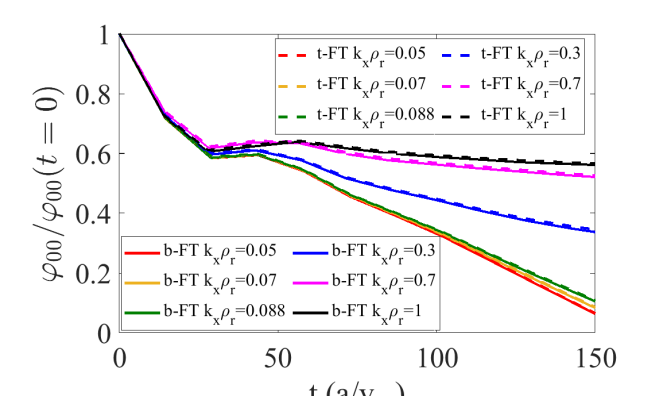

The residual zonal flow level is a long-time-scale property and it is questionable that this value can affect the nonlinear saturation of turbulence, which occurs in much shorter times. However, the short-time relaxation of the potential could more likely affect the saturation process. Here we look at the short-time scale behavior of the zonal potential decay in different computational domains. Figure 7 shows the short-time evolution of the zonal potential for several radial scales in simulations of ZF relaxation in the W7-X configuration for the two FTs with and that of the radial electric field222The electrostatic potential shows a similar, although noisier, time evolution than the electric field, which is the reason to use the later for fitting the model in Eq. 1 for extracting and . for several RG simulations with EUTERPE for different radial scales of the initial perturbation. At very short times, below the decay is almost independent of the radial scale of the perturbation in both computational domains, but for longer times, , it is clear that the short-time evolution changes with the radial scale as the residual level does. The similarity in the decay between both domains is remarkable. No significant differences are found in the short time decay of potential between FTs with different lengths in stella, while in GENE FT simulations a difference between FTs (not shown) is found for small values of the radial scale .
In conclusion, it is clear that short flux tubes are not sufficient to capture the long-term properties of the ZF relaxation, in general. Different flux tubes provide different results and they converge to the same result when the length of the FT is increased. The number of poloidal turns in the flux tubes that is required for convergence depends on the magnetic geometry and a general rule applicable to other magnetic configurations cannot be extracted from present practical cases. In the short-time evolution of the zonal potential less clear difference between flux tubes is found than in the long-term properties.
4 Linear stability of ITG modes
Now we turn our view to the ITG instability in different computational domains: FT, FFS and RG. We run simulations with adiabatic electrons and follow a similar approach to that employed in the previous section. Simulations for two stellarator-symmetric FTs with different lengths are compared with each other and also with FFS and RG simulations. We use the same codes, which provide different levels of information about the mode structure. Global codes run simulations with multiple modes whose radial structure can be extracted by Fourier transforming the radial mode structure in the post-processing. Full-flux-surface radially local simulations are multi-mode in the perpendicular direction along the flux surface, thus considering multiple scales. In the radial direction, GENE-3D contain also a number of different radial scales , determined by the box size. The radial structure of the modes could also, in principle, be extracted. In GENE, one single mode can be simulated. On the other hand, local linear FT simulations can scan the stability for each mode separately. With respect to the radial scale of the modes, in FT simulations, is set as a parameter and a set of simulations with different values of and has to be run in order to study how the linear instability depends on the radial scale.
The basic quantities to compare here will be the growth rate and the frequency of the ITG modes, which can be extracted from all the codes. The local FT codes can provide the growth rate and frequency for each pair separately, while from the RG and FFS simulations, eventhough they consider multiple modes, only the frequency and the linear growth rate of the most unstable mode considered in the simulation, which determines the growth of both mode and numerical noise amplitudes, can be extracted. Using the phase factor in EUTERPE, an estimate of the growth rates and frequencies of different modes can be scanned in a set of simulations in which the center of the Fourier filter is varied. For the comparison of wavenumbers the relation , with the poloidal mode number in PEST coordinates and the effective minor radius, is used. The values are normalized with the inverse Larmor radius, as usual. The growth rates and real frequencies are normalized to , with the ion thermal velocity.


The settings of the simulations are as follows. The electron temperature profile is flat, with , and density and ion temperature profiles, similar to those in [35] are used, which are given by the formula
| (2) |
where represents a radial profile of density () or ion temperature, , , , , , and and the minor radius. The profiles used in these simulations are shown in Figure 8. Two profiles of are shown; first, the one used in all the ITG simulations presented in Figures 9 and 11, with , shown with continuous thick line and labeled as “ref” in the figure; and also a profile, labeled as “narrow”, with , which has a smaller width of the profile. The local values at , , and , are used as input for the radially local simulations (FT and FS), all carried out at this radial position.
With these settings, linear simulations with adiabatic electrons are carried out in the standard configuration of LHD in the FT, FS and RG domains and the growth rate and the real frequency obtained in different domains with the different codes are compared. The numerical settings used in all the simulations in this section are given in Table 2.


Figure 9 shows the growth rate and frequency obtained in different computational domains in the LHD configuration at . FT simulations were carried out with both GENE and stella and the agreement between both codes is excellent. Only simulations in FTs with are shown in the Figure for clearness, but FTs with lengths provide almost exactly the same results for both and . FFS simulation results obtained with GENE333The FFS simulation with GENE has been carried out with because of technical reasons. and GENE-3D, and results from RG simulations with EUTERPE are also shown in this figure. In FFS and RG simulations only one point corresponding to the most unstable mode is represented. In the FFS simulation with GENE only one is resolved, while in GENE-3D a set of are resolved. The wider resolution simulation with EUTERPE (labeled as “WR” in the table) is full volume and covers the wavenumbers , which allows resolving modes up to . In addition to the full volume simulation, a scan in wavenumber has been carried out with EUTERPE. In this scan, the radial domain is limited to and the Fourier filter keeps modes with , with varied to scan different regions of the wavenumber spectrum. A FFS simulation was carried out with GENE-3D at r/a=0.5, with radially periodic boundary conditions, using the following resolution: and resolving modes . Here, are the number of points in the grids along the , , , and coordinates. For the RG simulation with GENE-3D, the radial domain was covered, the resolution was and covered the range . A very good agreement between all FTs and FFS domains is obtained, which can be explained by the smoothness and approximate periodicity along the magnetic field lines of the magnetic quantities in LHD. Figure 3 shows the magnetic field strength along a field line followed by the FT in the LHD configuration. The RG simulations provide a for the most unstable mode that is smaller than that obtained in FT or FFS simulations by 15-20%. The agreement in the mode frequency between all the codes/domains is very good.
| code domain | sim. | ||||||||||
|---|---|---|---|---|---|---|---|---|---|---|---|
| LHD | stella | FT | 0.5 | 1 | 1 | 128 | 48 | 24 | |||
| GENE | FT | 0.5 | 1 | 1 | 48 | 12 | |||||
| FFS† | 0.5 | 12 | 128 | 256 | 32 | 12 | |||||
| GENE-3D | FFS | 0.5 | 90 | 64 | 256 | 16 | 8 | ||||
| RG | 0.2-0.8 | 144 | 64 | 128 | 48 | 20 | |||||
| EUTERPE | RG∗ | LR | 127 | 0-1 | 64 | 256 | 64 | ||||
| scan | 63 | 0.31-0.7 | 96 | 64 | 32 | ||||||
| MHD | 0-1 | 141 | 256 | 256 | |||||||
| W7-X | stella | FT | 0.5 | 1 | 1 | 48 | 24 | ||||
| GENE | FT | 0.5 | 1 | 1 | 48 | 12 | |||||
| FFS | 0.5 | 12 | 256 | 128 | 32 | 12 | |||||
| FFS | 12 | 96 | 128 | 32 | 12 | ||||||
| GENE-3D | FFS | 0.5 | 90 | 384 | 128 | 32 | 8 | ||||
| 90 | 192 | 128 | 32 | 8 | |||||||
| 90 | 96 | 128 | 32 | 8 | |||||||
| EUTERPE | RG∗ | WR | 1023 | 0.31-0.7 | 256 | 1024 | 256 | ||||
| MR | 255 | 0-1 | 128 | 256 | 64 | ||||||
| scan | 34 | 0.31-0.7 | 128 | 64 | 64 | ||||||
| MHD | 0-1 | 99 | 256 | 256 | |||||||


Figures 10 and 11 show the comparison of and vs. the normalized wave number for FT, FFS and RG simulations in the KJM configuration of W7-X. Simulations for the two stellarator-symmetric FTs, (bean) and (triangular) with lengths , carried out with GENE and stella are shown in Figure 10. It is clear from the figure that in W7-X the situation is quite different from that for LHD, shown in Figure 9. The different FTs, with the shortest lengths (), provide different results for both and . The disagreement between short FTs is found both for the growth rate and the frequency. In the range the growth rates in different FTs are very similar but there is a clear disagreement in the frequencies, as highlighted in the inset of the bottom panel of Figure 10. In this region, a clear difference is also found in the radial scale of the most unstable modes for the bean and triangular FTs (see section 4.1). The difference in the results for short FTs can be traced back to the fact that the short bean and triangular FTs explore regions of the flux surface with very different properties (see Figures 1 and 2). As the length is increased, the FTs explore a larger region of the flux surface and the results from both FTs get closer, although bean and triangular FTs results do not match exactly even for large values of . Cases with and (not shown) demonstrate that good convergence with the length for each flux tube is found for with both stella and GENE, however, both FTs do not match with each other. Figure 11 shows the comparison of and in the W7-X configuration for the FT (), FFS and RG domains. A wavenumber scan with EUTERPE using the density and temperature reference profiles shown in Figure 8 and a small Fourier filter () is also shown in this figure, which qualitatively reproduces the wavenumber dependency from FT results, although with growth rates significantly smaller than those obtained for the bean FT in the region . In this scan, the radial domain is limited to . The scan in wavenumbers has been repeated, using the same numerical settings and the narrow profile from Figure 8 to check the influence of the width of the -profile, if any. For the narrow profile, only a slight reduction in is found while the general trend is kept. Finally, RG and FFS simulation results are shown with just a point per simulation, corresponding to the most unstable mode. Two more RG simulations with EUTERPE using the reference profiles and a wider resolution are shown. The simulation with the largest resolution (labeled as “WR” in the table) uses a Fourier filter keeping modes with , corresponding to , and cover the full radius. The medium resolution one (“MR” in the table) uses a filter keeping modes and . Three FFS simulations with different resolutions are shown for GENE-3D. The largest-resolution case, with resolutions , covers the wavenumbers , and for the others, the resolution is reduced by factors 2 and 4 and the largest wavenumbers resolved are and , respectively. Similar to what happens with EUTERPE simulations, the most unstable mode is found at wavenumbers increasing with resolution. Two FFS simulations carried out with GENE using different resolutions and resolving the maximum wavenumbers and 10.5, respectively, are also shown in the same figure. The relevant numerical settings used in all these simulations are given in Table 2. The results of GENE FFS simulations reasonably agree with FT simulations with GENE and stella showing a slightly larger growth rate. In GENE FFS simulations only the radial wavenumber is considered, while in GENE-3D a radial grid is used, which allows resolving a set of finite scales .


For , the results for FFS with GENE-3D and RG with EUTERPE reasonably coincide in the wavenumber of the most unstable mode, with close to that of the triangular FT and slightly smaller for FFS than for RG. In the range , both FFS and RG simulations give values of in between the most (triangular) and less unstable (bean) flux tubes. Interestingly, the peak in the growth rate found around by FT simulations is neither captured by the FFS nor the RG simulations.
For the frequencies, the agreement between all codes is very good for wavenumbers and for FTs with in both stella and GENE. In the range , the agreement between domains and between different FTs is not so good (see also Figure 10 for the detailed comparison of FTs).
The lack of periodicity of magnetic quantities along the field line in the W7-X configuration (see Figure 3) makes that different FTs give different results, in general. When the FT length is increased, the triangular flux tube results get close to those of the bean one. This is explained by the fact that for the triangular FT gets closer to the regions explored by the bean FT with , which finds the most unstable region around (see Figure 1, 2 and 3). A scan of FT simulations in the radial wavenumber (see section 4.1) shows that for the triangular FT, the most unstable mode is not always that of and that the scale of the modes at which the maximum growth rates are obtained changes with the FT length.
4.1 Dependence with the radial scale
In this section we study the radial scale of unstable ITG modes in FT simulations carried out with stella and compare them with RG simulations with EUTERPE. As described in section 2, in linear FT simulations is a parameter while in RG in RG, since the radial is not not a spectral coordinate, a continuum of radial scales is simulated.many radial scales are simulated at the same time. Then, in order to extract the dependence with for and in a FT, a scan in and has to be done. From a linear RG simulation, the radial scale for the most unstable mode is extracted by using a Fourier transform. We have computed the radial scale for the wavenumber scan shown in Figure 9 for LHD and a value is obtained for a wide range of wavenumbers . FT simulations with stella do not show a strong dependence of with either. In the W7-X configuration the situation is different, and a radial scale dependence on is found.


Figure 12 shows the growth rate in a scan in and carried out with stella in bean and triangular FTs with several lengths, for the KJM configuration of W7-X. For short flux tubes, different results are obtained for the bean and triangular one. The most unstable modes are located at in the bean flux tube, which is not the case for the triangular, where, unless the flux tube is extended so that it nearly overlaps with the bean flux tube, the most unstable mode is located at and . When the length is increased to these modes with and appear also in the bean FT with a large growth rate, even more clearly than in the triangular FT at any length.

In Figure 13, the radial scale of the most unstable modes is shown versus the normalized wavenumber for the scan performed with EUTERPE in the W7-X configuration shown in Figure 11. The radial scale is obtained by Fourier transforming the potential profile for the most unstable mode at each single simulation in the scan. In order to check to what extent the radial scale is affected by the profile, another simulation scan using a narrower profile (see Figure 8) was analyzed and the results (shown in Figure 13) are qualitatively the same in both cases. In this scan the values obtained for and were very close to those shown in Figure 11 for the reference scan.
In spite of the differences, a remarkable consistency between results from the global and FT simulations is found, and some important features are equally captured by both codes and computational domains. Firstly, for small wavenumbers the radial scale of the most unstable mode in the RG domain is small , in qualitative agreement with the results for the bean FT at short lengths, which shows the largest instability in this region of the maps. The radial wavenumbers of the unstable modes increase with up to around . Interestingly, these radial scales and are the most unstable in the triangular FT at in the region , while for they do not appear among the most unstable scales in the bean FT. For , the of the most unstable mode decreases to very small values around , which coincides qualitatively with the region in which the maximum growth rate is observed for small values of in both FTs in the maps from stella. In this region a local minimum in the growth rate was shown in Figures 10 and 11 which also appears in these maps. Finally, for the region an increase of for the most unstable mode with is obtained in the RG domain that seems to reflect the large spot in the maps from stella, particularly for the triangular FT, in which the maximum growth rate moves to regions of large values of for large . Given the differences between the FT and RG representations of the geometry, the consistency in results seems satisfactory.
The FT and RG domains provide different perspectives of the same 3D reality. The flux tubes sample a reduced region of the flux surface and are local in radius, while the RG simulation takes all the 3D structure into account. Consequently, one can expect that modes that are very unstable in a FT geometry can become screened when they are allowed to explore the full magnetic structure. The opposite situation can also be expected: modes that are not very unstable in a FT reduced domain can enhance its unstable properties when they explore larger regions of the flux surface/radius in the RG simulation. This effect appears when the triangular flux tube is extended from 1 to 3 poloidal turns, and the growth rate obtained increases up to similar values to those of the bean FT. Then, the picture obtained from a global simulation represents something “in between” the many FT that can be constructed in a flux surface.
5 Summary and conclusions
Two linear problems have been studied in gyrokinetic simulations carried out with different codes (GENE, GENE-3D, stella and EUTERPE) in different computational domains: flux tube, radially local full-flux-surface, and radially global domains. For the linear zonal flow relaxation problem, it has been shown that different flux tubes with the shortest length considered (one poloidal turn) give different results, in general. The results of different FTs get closer as their length is increased. Both the length required for convergence of FT results and the degree of convergence are configuration-dependent, in line with previous results [19]. In the particular case of LHD, different FTs give very similar results, which are also in reasonable agreement with RG and FFS simulations, particularly for small radial wavenumbers. However, in the W7-X configuration analyzed here the situation is very different and different FTs with one or two poloidal turns long provide different results for the long-term properties (ZF residual and oscillation frequency). For the ZF evolution at short times, no significant difference is found between FTs.
Not only the long-term properties but also the short-time evolution of the zonal structures show a dependency with the radial scale of the perturbation, which is in very good agreement between simulations in long-enough FTs and a RG domain.
Related to the ITG linear stability, the situation is somehow similar, but the growth rate of unstable modes captured by the FT local simulations is found to be dominated by the most unstable modes, with amplitude peaking at specific locations over the flux surfaces, which is in line with the strong localization of ITG (and also TEM) modes in stellarators found in previous works [36, 23, 37, 33]. In LHD, results of different flux tubes of any length match very well and are in good agreement with full surface or global simulation results. Radially global simulations are in very good agreement with FT and FFS in the frequency of the most unstable mode, but give a smaller (15-20%) growth rate. In W7-X, however, different flux tubes provide significantly different results for that get closer with each other as the FT length is increased, but they do not exactly match at any length .
The radial scale of unstable ITG modes shows a dependency with the binormal wavenumber in W7-X configuration, while in LHD only a weak dependency with was found. The dependency of the radial scale of the most unstable modes with in W7-X differs between FTs for short FT lengths. For long-enough flux tubes a qualitative consistency with radially global results is found in this respect, in spite of the differences between both computational domains.
The good agreement between different FTs, of any length, found in LHD for both the linear ITG instability, and for the linear ZF evolution, cannot be considered a situation valid for other devices, in general. The results for the W7-X configuration, as well as previous results in quasisymmetric devices [19], show that the convergence between results from different flux tubes is configuration-dependent. Furthermore, the sampling of the flux surface by flux tubes of increasing lengths is largely conditioned by the rotational transform. Besides, the situation for other different instabilities, such as trapped electron modes, which can be located preferentially at different locations than those where the ITG modes, can be very different.
FFS and RG results are in reasonable agreement, which indicates that the FFS simulation domain can be considered the minimum appropriate computational domain for stellarators. However, slight differences between simulations in these domains appear.
Work is in progress to study how the linear stability and zonal flow evolution studied here translate in simulations of nonlinearly saturated ITG turbulence in stellarators.
6 Acknowledgements
Simulations were carried out in Mare Nostrum IV and Marconi supercomputers. We acknowledge the computer resources and the technical support provided by the Barcelona Supercomputing Center and the EUROfusion infraestructure at CINECA. The work has been partially funded by the Ministerio de Ciencia, Innovación y Universidades of Spain under project PGC2018-095307-B-I00. This work has been carried out within the framework of the EUROfusion Consortium and has received funding from the Euratom research and training programme 2014-2018 and 2019-2020 under grant agreement No 633053. The views and opinions expressed herein do not necessarily reflect those of the European Commission.
7 References
References
- [1] Beer, M. A. et al. Phys. Plasmas 2 (1995) 2687.
- [2] Martin, M. F. et al. Plasma Phys. Control. Fusion 60 (2018) 095008.
- [3] Faber, B et al. Phys. Plasmas 22 (2015) 072305.
- [4] Mishchenko, A. et al. Physics of Plasmas, 15(7) (2008) 72309.
- [5] Helander, P. et al. Plasma Phys. Control. Fusion 53 (2011) 054006.
- [6] Monreal, P. et al. Plasma Phys. Control. Fusion 58 (2016) 045018.
- [7] Plunk, G. et al. Physical Review Letters, 118(10) (2017).
- [8] Villard, L., Bottino A.,Sauter O. et al. Phys. Plasmas, 9(6), 2684 (2002)
- [9] Riemann, J. et al. Plasma Physics and Controlled Fusion, 58(7)(2016) 74001.
- [10] Jost, G. et al. Physics of Plasmas, 8(7) (2001) 3321.
- [11] Barnes, M. et al. Journal of Computational Physics 391 (2019) 365.
- [12] Jenko, F. et al. Phys. Plasmas 7 (2000) 1904.
- [13] Maurer, M. et al. J. Comput. Phys. 420, 1 (2019).
- [14] Sugama, H. and Watanabe T-H Phys. Rev. Lett. 94 (2005) 115001.
- [15] Sugama, H. and Watanabe, T. H. Phys. Plasmas 13 (2006) 012501.
- [16] Sugama, H and Watanabe, T. H. Phys. Plasmas 14 (2007) 079902.
- [17] Mynick, H. E. and Boozer, A H Phys. Plasmas 14 (2007) 072507.
- [18] Monreal, P. et al. Plasma Phys. Control. Fusion 118 (2017) 185002.
- [19] Smoniewski. J. et al. Phys. Plasmas 28, (2021) 042503.
- [20] Grimm, R. C., et al. J. Comput. Phys. 49, 94 (1983).
- [21] Sánchez E. et al. Relaxation of zonal flows in stellarators: influence of the magnetic configuration. Proc. of the 42nd European Physical Society Conference on Plasma Physics, Lisbon, Portugal, June 2015.
- [22] Xanthopoulos P., Cooper W A, Jenko F, Turkin Yu, Runov A and Geiger J. Phys. Plasmas 16 (2009) 082303.
- [23] Kornilov, V. et al. Phys. Plasmas 3196 (6) (2004).
- [24] Slaby, C. et al. Nuclear Fusion 58 (2018) 082018.
- [25] Hirshman, S. P. et al. Phys. Fluids 26 (1983) 3553.
- [26] Pueschel M. J., Dannert T. and Jenko F. Comput. Phys. Commun. 181 (2014) 1428.
- [27] Kleiber, R. et al. Contrib. Plasma Phys. 50 (2010) 766.
- [28] Sánchez, E. et al. Plasma Phys. Control. Fusion 55 (2013) 014015.
- [29] Xanthopoulos, P. et al Physical Review Letters 107 (2014) 245002.
- [30] Alonso, J. A. et al. Phys. Rev. Lett. 118 (2017) 185002.
- [31] Mishchenko, A. and Kleiber, R. Phys. Plasmas 19, (2012) 072316.
- [32] Sánchez, E. et al. Plasma Physics and Controlled Fusion 60 (9) (2018) 094003.
- [33] Sánchez, E. et al. Nucl. Fusion 59 (2019) 076029.
- [34] Winsor, N. et al. Phys. Fluids 11 (1968) 2448.
- [35] Sánchez, E. et al. J. Plasma Phys., vol. 86 (2020)855860501.
- [36] Nadeem, M. et al. Phys. Plasmas, 8(10 (2001) 4375.
- [37] Xanthopoulos, P. et al. Physical Review Letters, 113(15) (2014) 155001.
- [38] Diamond, P. H,, Itoh, S. I. and Itoh, K. and Hahm, T. S. Plasma Phys. Control. Fusion 47(5) (2005).