Guaranteed Multidimensional Time Series Prediction via Deterministic Tensor Completion Theory
Abstract
In recent years, the prediction of multidimensional time series data has become increasingly important due to its wide-ranging applications. Tensor-based prediction methods have gained attention for their ability to preserve the inherent structure of such data. However, existing approaches, such as tensor autoregression and tensor decomposition, often have consistently failed to provide clear assertions regarding the number of samples that can be exactly predicted. While matrix-based methods using nuclear norms address this limitation, their reliance on matrices limits accuracy and increases computational costs when handling multidimensional data. To overcome these challenges, we reformulate multidimensional time series prediction as a deterministic tensor completion problem and propose a novel theoretical framework. Specifically, we develop a deterministic tensor completion theory and introduce the Temporal Convolutional Tensor Nuclear Norm (TCTNN) model. By convolving the multidimensional time series along the temporal dimension and applying the tensor nuclear norm, our approach identifies the maximum forecast horizon for exact predictions. Additionally, TCTNN achieves superior performance in prediction accuracy and computational efficiency compared to existing methods across diverse real-world datasets, including climate temperature, network flow, and traffic ride data. Our implementation is publicly available at https://github.com/HaoShu2000/TCTNN.
Index Terms:
multidimensional time series, prediction, deterministic tensor completion, temporal convolution low-rankness, exact prediction theoryI Introduction
Multidimensional time series, characterized by data with two or more dimensions at each time point, are often generated in a wide range of real-world scenarios, such as regional climate data [1], network flow data [2], video data [3], international relations data [4], and social network data [5]. Accurate forecasting of these temporal datasets is critical for numerous applications [6] [7] [8], such as optimizing route planning and traffic signal management in intelligent transportation systems [9] [10]. Affected by the acquisition equipment and other practical factors, the length of the observation data may be limited. For instance, high-throughput biological data, such as gene expression datasets, typically contain numerous features but only a few time samples [11]. Therefore, developing reliable few-sample multidimensional time series prediction methods has been a long-standing basic research challenge.
Traditional time series models, such as vector autoregression [12] and its variants [13] [14] [15], are not well-suited for handling multidimensional data. Recent studies represent multidimensional time series as tensors [5], where the first dimension corresponds to time and the remaining dimensions capture features or locations. For example, temperature data across different geographical locations can be structured as a third-order tensor (time × longitude × latitude), inherently preserving interactions between dimensions [16]. This tensor representation has enabled the development of methods such as tensor factor models [5] [17] and tensor autoregressive models [18] [19] [20] [21].
Another promising approach is to frame multidimensional time series prediction as a tensor completion task, where the regions of interest are treated as missing values. As illustrated in Fig.1, this process involves three steps: concatenating observed and predicted time series into an incomplete tensor, completing the tensor, and extracting the forecasted values. Within this framework, the low-rankness of multidimensional time series has been extensively utilized, leading to decomposition-based forecasting methods [1] [22] [23]. Nevertheless, existing tensor factorization, autoregressive, and decomposition models fail to offer a definitive conclusion about the number of samples that can be predicted exactly.

Low-rank tensor completion methods based on nuclear norm minimization, supported by recovery theory, offer a promising alternative. Some researchers have converted multidimensional time series into matrices and applied deterministic matrix nuclear norm minimization theories for predictive modeling [24] [25] [26] [27]. While these approaches provide theoretical support, they suffer from two key limitations: (1) the conversion from tensors to matrices loses critical structural information, reducing prediction accuracy; and (2) the computation of large-scale matrix nuclear norms imposes significant computational and memory costs. Despite advances in deterministic matrix recovery theory, an equivalent theory for tensor nuclear norm minimization remains absent, necessitating such matrix-based approaches [28, 29, 30, 31, 32, 33, 34, 35, 36, 37].
To address this gap, we propose a deterministic tensor completion theory based on tensor nuclear norm minimization for non-random missing data. Unlike direct application of tensor nuclear norm minimization to forecasting, our method introduces a Temporal Convolution Tensor Nuclear Norm (TCTNN) model, which transforms multidimensional time series via temporal convolution and applies tensor nuclear norm minimization to the transformed data. This approach establishes an exact prediction theory while achieving higher accuracy and lower computational costs compared to existing methods. Our main contribution can be summarized as follows:
-
•
Within the t-SVD framework, a tensor completion theory suitable for any deterministic missing data has been established by introducing the minimum slice sampling rate as a new sampling metric.
-
•
The TCTNN model is proposed by encoding the low-rankness of the temporal convolution tensor, and its corresponding exact prediction theory is also provided. Furthermore, the impact of the smoothness and periodicity of the time dimension on the temporal convolution low-rankness is analyzed.
-
•
The proposed TCTNN model is efficiently solved based on ADMM framework and well tested on several real-world multidimensional time series datasets. The results indicate that the proposed method achieves better performance in prediction accuracy and computation time over many state-of-the-art algorithms, especially in the few-shot scenario.
The remainder of this paper is organized as follows. In Section II, we review a series of related works. In Section III, A deterministic tensor completion theory is establish. Section IV gives the proposed TCTNN method and its corresponding prediction theory, and Section V introduces the optimization algorithm. In Section VI, we conduct extensive experiments on some multidimensional time series datasets. Finally, the conclusion is given in Section VII. It should be noted that all proof details are given in supplementary materials.
II Related Works
II-A Deterministic completion theory
Recovery theory for matrix/tensor completion in random cases has been extensively studied, yielding significant advancements in many fields [38] [39] [40] [41]. In contrast, deterministic observation patterns have garnered considerably less attention. However, the pattern of missing entries depends on the specific problem context in practice, which can lead to highly non-random occurrences. A case in point is the presence of missing entries in images, which is often attributed to occlusions or shadows present in the scene. To investigate the recovery theory for matrix/tensor completion under non-random missing conditions, previous researchers have conducted extensive exploration using various tools [28, 29, 30, 31, 32, 33, 34, 35, 36, 37]. For instance, Singer et al. [29] apply the basic ideas and tools of rigidity theory to determine the uniqueness of low-rank matrix completion. Based on Plücker coordinates, Tsakiris [31] provides three families of patterns of arbitrary rank and arbitrary matrix size that allow unique or finite number of completions. Besides, Liu et al. [36] propose isomeric condition and relative well-conditionedness to ensure that any matrix can be recovered from sampling of matrix terms. Despite these advancements, most of the current theoretical work focuses on deterministic matrix completion, while the tensor case is not explored enough. Therefore, the theoretical framework for deterministic tensor completion still requires significant enhancement.
II-B Time series prediction via matrix/tensor completion
Matrix and tensor completion methods have garnered significant attention for time series forecasting [23] [26] [42]. These approaches generally fall into two categories: decomposition-based methods and nuclear norm-based methods. Matrix/tensor decomposition, widely used for collaborative filtering, provide a natural solution for handling missing data in time series forecasting [42] [43] [44]. These models approximate the incomplete time series using bilinear or multilinear decompositions with predefined rank parameters. To capture temporal dynamics, recent studies have introduced temporal constraint functions, such as autoregressive regularization terms, to regularize the temporal factor matrix [45] [23] [44]. Based on this, Takeuchi et al. [22] model spatiotemporal tensor data by introducing spatial autoregressive regularizer, providing additional predictive power in the spatial dimension.
As opposed to decomposition-based methods, nuclear norm-based approaches do not require predefined rank parameters [38] [40] [41]. However, directly applying nuclear norms to time series often yields suboptimal predictions [6]. A practical enhancement involves applying structural transformations to time series data to create structured matrices, enabling the application of nuclear norms for forecasting. For example, Gillard et al. [26] and Butcher et al. [27] used the Hankel transform to convert univariate time series into Hankel matrices and applied nuclear norm minimization for prediction. Similarly, Liu et al. [24] [25] utilized convolution matrices for encoding nuclear norms, providing insights into the predictive domain that can be exactly forecasted. Although these methods offer predictive insights, they involve converting time series into large matrices, resulting in the loss of inherent tensor structure and imposing high computational costs. To address these limitations, we propose the Temporal Convolution Tensor Nulclear Norm (TCTNN) model, which preserves the tensor structure, offers theoretical guarantees for predictions, and achieves superior performance in terms of both accuracy and computational efficiency.
III Deterministic Tensor Completion
In contrast to the typical scenario of tensor completion with random missing values, the prediction problem in the context of multidimensional time series prediction corresponds to a deterministic tensor completion problem. To address this, we first introduce a new theory of deterministic tensor completion in this section.
III-A T-SVD Framework
We begin by providing a brief overview of the key concepts within the tensor Singular Value Decomposition (t-SVD) framework [46] [47] [48] [49] [50]. This includes the tensor-tensor product, tensor nuclear norm, and the conditions for tensor incoherence. Following this, we propose a novel deterministic sampling metric designed to establish an exact recovery theory for deterministic tensor completion.
For consistency, we use lowercase, boldface lowercase, capital, and Euler script letters to represent scalars, vectors, matrices, and tensors, respectively, e.g., , , , and . For an order- tensor of dimensions , its elements, slices, and sub-tensors are represented as , such as represents the -th element and represents the -th face slice. To construct the t-SVD framework, some operators on are summarized in Table I.
| Notations | Descriptions |
|---|---|
| , | |
| size | |
| , | |
| size | |
| , | |
| size | |
| , | |
| size | |
| the inverse operation of | |
| , | |
| size |
Definition III.1 (T-product [49]).
Let order- tensors and , then the t-product is defined to be a tensor of size ,
| (1) |
Definition III.2 (Circular convolution [51]).
For any tensors and with , the circular convolution of two tensors is
| (2) |
or element-wise,
| (3) |
where denotes the circular convolution operator. The circulant boundary condition are satisfied by assuming with if and otherwise, .
Since the multiplication of and is in the form of circular convolution, t-product can also be defined using circular convolution:
| (4) |
where denotes the operator of circular convolution. Evidently, the t-product of tensors is an operation analogous to matrix multiplication. As a result, many properties of matrix multiplication can be extended to the t-product [48] [50].
In addition, the discrete Fourier transform (DFT) can convert the circular convolution operation into an element-wise product. Therefore, the t-product can be obtained through DFT. For a given tensor , its Fourier-transformed in last d-2 dimensions is expressed as
| (5) |
where denotes the j-mode product [52] and represents the DFT matrices of size for . Then
| (6) |
where denotes the face-wise product ( for all face slices).
Definition III.3 (Identity tensor [49]).
The identity tensor is the tensor with its first face slice being the identity matrix and the other face slices being all zeros.
Definition III.4 (Transpose [49]).
For an order- tensor , its transpose is the obtained by tensor transposing each for and then reversing the order of the through .
Definition III.5 (Orthogonal tensor [49]).
An order- tensor is orthogonal if , where is an order- identity tensor.
Definition III.6 (F-diagonal tensor [49]).
A tensor is said to be f-diagonal if all of its face slices are diagonal.
Lemma III.1 (T-SVD [49]).
Let tensor , then it can be factorized as
| (7) |
where , are orthogonal tensors, and is a f-diagonal tensor.
Definition III.7 (Tensor tubal rank) [48] [50]).
For with t-SVD , its tubal rank is defined as
where denotes the cardinality of a set.
Definition III.8 (Tensor multi-rank [48] [50]).
The multi-rank of a tensor is represented by a vector . The -th element of corresponds to the rank of the -th block of . We denote the tensor multi-rank sum as , which means .
Definition III.9 (Tensor spectral norm [48] [50]).
For order- tensor , its tensor spectral norm is defined as
where denotes the spectral norm of a matrix or tensor.
III-B Deterministic Tensor Completion
Now we consider deterministic tensor completion problem, a broader research challenge. Let represent an unknow target tensor with tubal rank and skinny t-SVD . Suppose that we observe only the entries of over a deterministic sampling set . The corresponding mask tensor is denoted by , with the following entry definition:
The sampling operator is then defined as where denotes the Hadamard product.

To address the deterministic tensor completion problem, we employ a standard constrained Tensor Nuclear Norm (TNN) model:
| (9) |
where is a deterministic sampling set. In the context of tensor completion under random sampling, it is often assumed that the data sampling follows a specific distribution, such as the Bernoulli distribution, then the sampling probability can naturally serve as a measure of sampling [48]. However, this approach is clearly ineffective for deterministic sampling. Inspired by the minimum row/column sampling ratio for matrix deterministic sampling [36], we introduce a tensor deterministic sampling metric , termed the minimum horizontal/lateral sub-tensor sampling ratio. Here, the horizontal/lateral sub-tensors of a tensor are analogous to the rows/columns of a matrix, respectively. As mentioned above, the tensor t-product, spectral/nuclear norm within the t-SVD framework are defined in a matrix-like manner, providing a solid basis for defining tensor deterministic sampling metric by following matrix case.
Definition III.11 (Horizontal/lateral mask sub-tensor sampling number).
For any fixed sampling set with corresponding mask tensor , the -th horizontal mask sub-tensor, i,e., the -th horizontal sub-tensor of mask tensor, is given as . The -th horizontal mask sub-tensor sampling number is then defined as
Similarly, following , the -th lateral mask sub-tensor sampling number is defined as
where denotes the cardinality of a set.
For an intuitive understanding, we provide a schematic diagram illustrating horizontal/lateral mask sub-tensor sampling number in the three-dimensional case, as shown in Fig.2.
Definition III.12 (Minimum horizontal/lateral sub-tensor sampling ratio).
For any fixed sampling set , its minimum horizontal/lateral sub-tensor sampling ratio is defined as the smallest fraction of sampled entries in each horizontal and lateral mask sub-tensor; namely,
| (10) |
where .
Tensor incoherence is a crucial theoretical tool in low-rank tensor recovery [38] [39] [50] [53]. It enforces or constrains the low-rank structure of the underlying tensor to avoid ill-posed problems, such as when most elements of are zero, yet it is still low-rank.
Definition III.13 (Tensor incoherence conditions [50]).
For with tubal rank and it has the skinny t-SVD , and then is said to satisfy the tensor incoherence conditions with parameter if
| (11) |
| (12) |
where , is the order- tensor mode-1 basis sized , whose -th entry equals 1 and the rest equal 0, and is the mode-2 basis.
III-C Exact Recovery Guarantee
We briefly show the exact recovery guarantee of deterministic low-rank tensor completion problem.
Theorem III.1.
Suppose that obeys the standard tensor incoherence conditions (11)-(12), and is its minimum horizontal/lateral sub-tensor sampling ratio. if
| (13) |
where is the tubal rank of tensor , is the multi-rank sum and is the parameter of tensor incoherence conditions , then is the unique solution to the TNN model (9).
The above result demonstrates that minimizing the tensor nuclear norm can achieve exact deterministic tensor completion, provided that condition (13) is satisfied. The feasibility of exact recovery hinges upon the interplay between the sampling set and the tensor rank. As the low-rank structure of the tensor strengthens, the minimum slice sampling ratio required for exact deterministic tensor completion decreases correspondingly. Moreover, the proposed deterministic exact recovery theory can be extended to the random sampling case. The following corollary reveals that when the sampling set satisfies and , exact recovery holds with high probability.
IV Multidimensional Time Series Prediction
Let us denote the multidimensional time series as , where . The objective is to predict the next unseen samples given the historical portion , where represents the number of samples in the time dimension and denotes the number of samples to be predicted, referred to as the forecast horizon.
IV-A Time series prediction via TNN
Multidimensional time series prediction, as a specific instance of deterministic tensor completion, can be addressed using the aforementioned tensor nuclear norm minimization, which results in the following model:
| (14) |
where represents the deterministic sampling set corresponding to the historical portion sample, is the projection operator. denotes the multidimensional time series to be completed.
Deterministic tensor completion theory can be applied to prediction tasks where the sampling set is chosen as the historical data region in the prediction problem. However, in such cases, the minimum horizontal/lateral sub-tensor sampling ratio
| (15) |
which fails to meet the recovery conditions (13). This implies that tensor nuclear norm minimization cannot be directly applied to prediction tasks, as it would result in prediction outcomes that are entirely zero. The core issue lies in the concentrated nature of missing data in time series forecasting, which leads to insufficient sampling coverage. A natural solution to this problem is to implement a structural transformation that disperses the missing data, thereby increasing the minimum horizontal/lateral sub-tensor sampling ratio above zero. To address this, we introduce the temporal convolution tensor for multidimensional time series. This approach ensures that each horizontal/lateral sub-tensor contains a sufficient number of sampled elements, as illustrated in Fig.3.
IV-B Temporal Convolution Tensor
In this study, circular convolution (III.2) is applied only along the time dimension of the multidimensional time series, a process referred to as temporal circular convolution. Following this, we obtain the temporal convolution tensor of the multidimensional time series.
Definition IV.1 (Temporal circular convolution operator).
The temporal circular convolution procedure of converting and into is expressed as follows:
| (16) |
where denotes the temporal circular convolution operator, is the kernel vector, and it is assumed that for , which is the temporal circulant boundary condition.
Definition IV.2 (Temporal Convolution Tensor).
The temporal convolution tensor of multidimensional time series can be obtained via temporal circular convolution:
| (17) |
where denotes the temporal circular convolution operator, is the temporal convolution transform, and the temporal convolution tensor is given by:
where represents the information of multidimensional time series at the -th time sampling point, in other words, .
Definition IV.3 (Temporal convolution sampling set).
For a sampling set of prediction problem , its temporal convolution sampling set is denoted by and given by
| (18) |
where is the mask tensor of and is the mask tensor of . Note that the consistency between sampling after transformation and transformation after sampling: , where ,
To provide an intuitive understanding, we present a schematic diagram illustrating the conversion from a multidimensional time series (incomplete tensor) of size to the corresponding temporal convolution tensor of size , as shown in Fig.3(a,b). Notably, the last horizontal sub-tensor of the incomplete tensor consists entirely of zeros. However, after applying the temporal convolution transform , each horizontal and lateral slice of the incomplete temporal convolution tensor contains a sufficient number of sampled entries. As depicted in Fig.3(b), the temporal convolution sampling set achieves a minimum horizontal/lateral sub-tensor sampling ratio
| (19) |
This significantly disperses the unobserved regions, enhancing the potential for axact predictions.

IV-C Temporal Convolution Tensor Low-rankness from Smoothness and Periodicity

By applying transform to the incomplete multidimensional time series , we obtain the incomplete temporal convolution tensor with a relatively dispersed distribution of missing values. In many cases, the completion of a tensor relies on its low-rankness, and this holds true for the temporal convolution tensor as well. Fortunately, The low-rankness of the temporal convolution tensor can often be satisfied in various scenarios, as it can be derived from the smoothness and periodicity of the time series . To reach a rigorous conclusion, we consider the rank-r approximation error of temporal convolution tensor , which is denoted by and defined as
where .
Lemma IV.1.
We can find an indicator to represent the strength of the smoothness of tensor along the temporal dimension, which can be defined as
then
Lemma IV.2.
If the approximate period is , we can find an indicator to represent the strength of the periodicity of tensor along the time dimension, which can be defined as
where for then
The notation in aboves lemmas denotes the ceiling operation. Lemma IV.1 and Lemma IV.2 indicate that as the periodicity and smoothness of the original data matrix/tensor along the time dimension increase, the low-rankness of its temporal convolution tensor becomes more pronounced. To illustrate this concept intuitively, we generated two multivariate time series: one exhibiting strong periodicity and the other characterized by temporal smoothness, as shown in Fig.4(a-1,a-2), respectively. Temporal convolution transform were applied to these time series matrices, and the resulting temporal convolution tensors are depicted in Fig.4(b-1,b-2). As shown in Fig.4(c-1,c-2), the tensor singular values of the temporal convolution tensors decrease rapidly. This trend highlights the enhanced low-rankness of the temporal convolution tensors, further substantiating the theoretical findings.
IV-D Temporal Convolution Tensor Nulclear Norm
Given that the smoothness and periodicity of the original time series tensor ensure the low-rank property of the temporal convolution tensor , it is natural to leverage the convex relaxation of tensor rank—the tensor nuclear norm—to encode this low-rankness. This leads to the formulation of the following completion model:
| (20) |
to obtain as the estimator of . After that, we perform the inverse temporal convolution on , thereby obtaining as the final preditior of .
This logical flow is depicted in Fig.3, outlining the steps to obtain the complete tensor from the incomplete tensor in the prediction problem. The process consists of three main steps: 1.Transformation: Apply the temporal convolution transform to the incomplete tensor , resulting in the incomplete temporal convolution tensor P; 2. Completion: Solve model (20) to derive the complete temporal convolution tensor from the incomplete tensor ; 3. Inverse Transformation: Retrieve the complete tensor by applying the inverse transform . By consolidating these steps into an equivalent representation, we formulate the Temporal Convolution Tensor Nuclear Norm (TCTNN) model for multidimensional time series prediction, i.e.,
| (21) |
where and is the forecast horizon.
IV-E Exact Prediction Guarantee
We now develop the exact prediction gaurantee for time series data prediction by applying the deterministic tensor completion theory established in the preceding section. We first define the temporal convolution tensor incoherence conditions as follows:
Definition IV.4 (Temporal convolution tensor incoherence).
For , assume that the temporal convolution tensor with tubal rank and it has the skinny t-SVD , and then is said to satisfy the temporal convolution tensor incoherence conditions with kernel size and parameter if
| (22) |
| (23) |
where , is the order- tensor sized , whose -th entry equals 1 and the rest equal 0, and .
Based on the temporal convolution tensor incoherence, we derive the exact prediction theory for the TCTNN model (21) from the deterministic tensor completion recovery theory.
Theorem IV.1.
Suppose that obeys the temporal convolution tensor incoherence conditions (22)-(23) with kernel size k. If
| (24) |
where is the tubal rank of tensor , is the multi-rank sum of tensor and is the parameter of temporal convolution tensor incoherence conditions, then is the unique solution to the TCTNN model (21).
Theorem IV.1 states that exact prediction is promising when the temporal convolution low-rankness is satisfied. As the low-rankness of the temporal convolution tensor increases and the prediction horizon decreases, achieving exact predictions becomes increasingly feasible. According to Lemmas IV.2 and IV.1, stronger periodicity and smoothness in the temporal dimension contribute to greater low-rankness in the temporal convolution tensor, thereby improving the likelihood of exact prediction.
IV-F Comparison with the CNNM model
In very recent, Liu et al. [25] propose the convolution matrix nulclear norm minimization (CNNM) model which can be formulated as
| (25) |
where is kernel size, represents the time series to be completed, denotes the nuclear norm of a matrix and denotes the transformation that converts the time series into the convolution matrix.
In contrast to the CNNM model, the proposed TCTNN model does not convert the original data tensor into convolution matrices along each dimension. Instead, we perform tensor convolution along the temporal dimension of the time series data. Our approach offers advantages in three aspects. 1. Tensor structure information: It preserves the tensor structure of multi-dimensional time series and avoids the information loss caused by converting tensor data into matrices. As demonstrated by the fact that , our temporal convolution tensors maintain the structure information of the multidimensional time series, unlike the convolution matrices, which satisfy . 2. Computational complexity: It avoids the computationally expensive task of processing the nuclear norm of very large matrices, significantly reducing the computational cost. For example, to predict a -order multidimensional time series , the computational complexity of each iteration of the CNNM model is , while the TCTNN model requires only per iteration. Clearly, the computational complexity of the former is nearly prohibitive. 3. Feature utilization: By performing convolution exclusively along the time dimension, our method is better suited for time series data. Many time series exhibit strong characteristics such as periodicity and smoothness only along the time dimension. Convolution along all dimensions could lead to improper feature capture, thereby reducing prediction accuracy.
V Optimization Algorithm
This section gives the optimization algorithm of the proposed TCTNN model (21) for the multidimensional time series prediction task.
V-A Optimization to TCTNN
We adopt the famous optimization framework alternating direction method of multipliers (ADMM) [54, 55, 56] to solve the model (21). First of all, we introduce the auxiliary variable to separate the temporal convolution transform , then the TCTNN model (21) can be rewritten as below:
| (26) | ||||
For model (26), its partial augmented Lagrangian function is
| (27) | ||||
where are Lagrange multipliers, is a positive scalar, and is only the multipliers dependent squared items. According to the ADMM optimization framework, the minimization problem of (27) can be transformed into the following subproblems for each variable in an iterative manner, i.e.,
| (28) |
| (29) | ||||
| s.t. |
and the multipliers is updated by
| (30) |
where denotes the count of iteration in the ADMM. In the following, we deduce the solutions for (28) and (29) respectively, each of which has the closed-form solution.
1) Updating : Fixed other variables in (28), then it degenerates into the following tensor nuclear norm minimization with respect to , i.e.,
| (31) |
the close-form solution of this sub-problem is given as
| (32) |
via the order- t-SVT as stated in Lemma III.2.
2) Updating : By deriving simply the KKT conditions, the closed-form solution of (29) is given by
| (33) |
where is the complement of and is the inverse operator of . The whole optimization procedure for solving proposed TCTNN model (21) is summarized in Algorithm 1.
V-B Computational Complexity Analysis
For Algorithm 1, the computational complexity in each iteration contains three parts, i.e., steps . First, the time complexity for order- t-SVT in step 3 is , corresponding to the linear transform and the matrix SVD, respectively [50]. The steps 4 and 5 have the same complexity with only element-wise computation. In all, the pre-iteration computational complexity of Algorithm 1 is .
V-C Convergence Analysis
Using optimality conditions and the saddle point theory of the Lagrangian function, we derive the following convergence theory for Algorithm 1.
VI Experimental results
In this section, we present a comprehensive experimental evaluation of the proposed temporal convolution tensor nulclear norm (TCTNN) approach using several real-world multidimensional time series datasets.
VI-A Multidimensional Time Series Datasets
Throughout the experiments, we adopt the following three real-world multidimensional time series datasets which are widely used in peer works.
-
1.
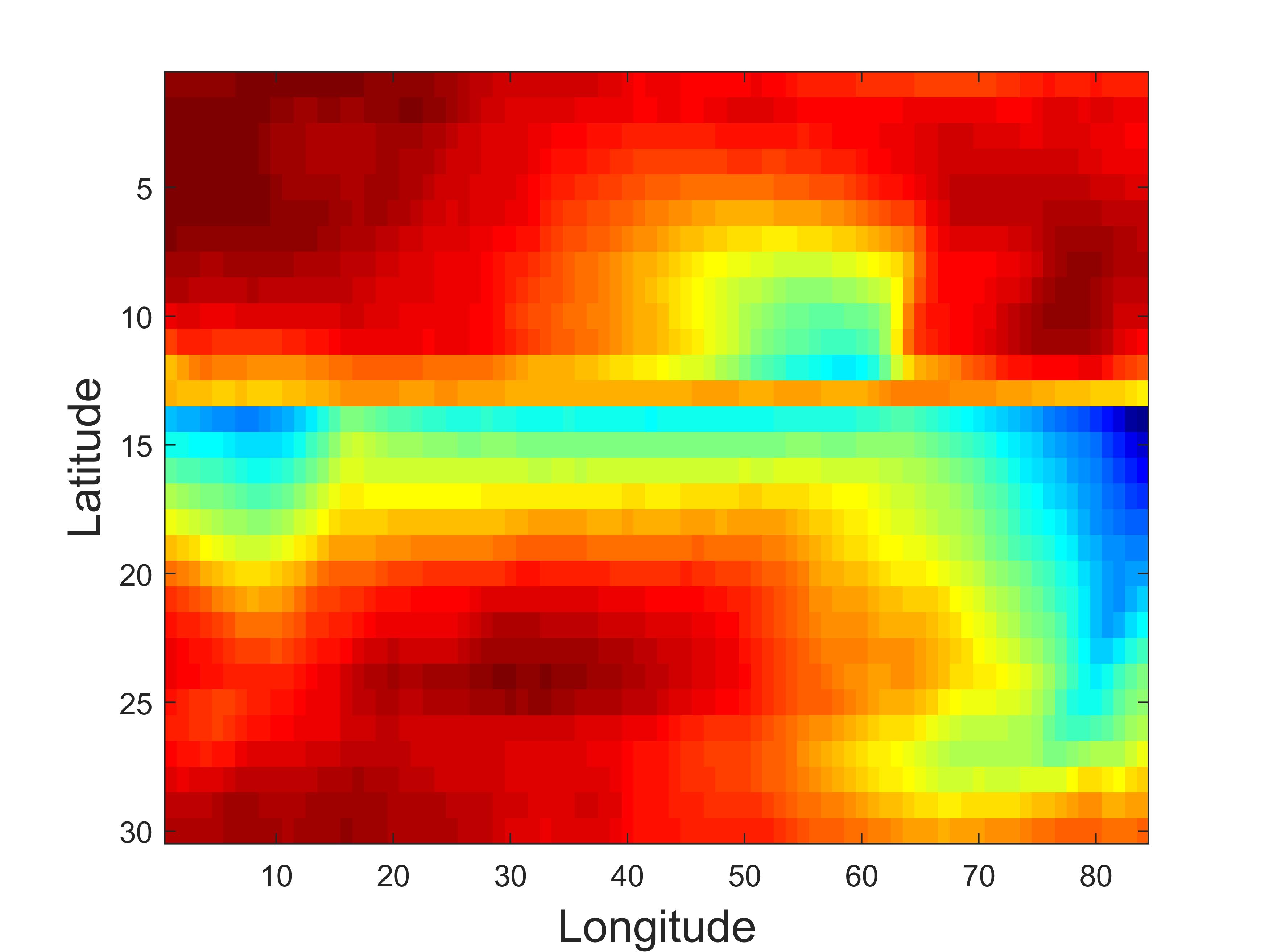
Pacific: The Pacific surface temperature dataset111http://iridl.ldeo.columbia.edu/SOURCES/.CAC/. This dataset is sourced from sea surface temperature on the Pacific over 50 consecutive months from January 1970 to February 1974. The spatial locations are represented by a grid system with a resolution of 2 × 2 latitude-longitude. The grid comprises 30 × 84 cells, resulting in a three-dimensional temperature data tensor with dimensions of 50 × 30 × 84, where 50 corresponds to the temporal dimension, while 30 and 84 represent the latitudinal and longitudinal grid counts, respectively.
-
2.
Abilene: The Abilene network flow dataset222http://abilene.internet2.edu/observatory/data-collections.html. Regarding the Abilene dataset, it encompasses 12 routers. Network traffic data for each Origin-Destination (OD) pair is recorded from 12:00 AM to 5:00 AM on March 1, 2004, with a temporal resolution of 5 minutes. We structure this data into a tensor with dimensions 60 × 12 × 12, where the first mode represents 60 time intervals, the second mode denotes 12 source routers, and the third mode signifies 12 destination routers.
-
3.
NYC taxi: The New York taxi ride information Dataset333https://www1.nyc.gov/site/tlc/about/tlc-trip-record-data.page. For the experimental phase, we selected trip data collected from 12:00 AM on May 1st to 02:00 AM on May 3rd, 2018. The raw data is subsequently organized into a third-order tensor, structured as (pick-up zone × drop-off zone × time slot). We delineate a total of 30 distinct pick-up/drop-off zones, and adopt a temporal resolution of 1 hour for trip aggregation. Consequently, the resulting spatiotemporal tensor exhibits dimensions of 50 × 30 × 30.
VI-B Baseline Methods
To evaluate the proposed TCTNN method, we compare it with the following baselines:
-
1.
SNN: The Sum of Nuclear Norms [3]. This Low-Rank Tensor Completion (LRTC) method employs the minimization of the sum of nuclear norms of unfolded matrices of tensors to accurately estimate unobserved or missing entries in tensor data.
-
2.
TNN: Tensor Nuclear Norm [53]. This method achieves low-rank tensor completion by minimizing the tensor nuclear norm, thereby facilitating the reconstruction of missing data.
-
3.
BTTF: Bayesian Temporal Tensor Factorization [1]. This method employs tensor factorization and incorporates a Gaussian Vector Autoregressive (VAR) process to characterize the temporal factor matrix.
-
4.
BTRTF: Bayesian Temporal Regularized Tensor Factorization [23]. The temporal regularized matrix factorization (TRMF) method discussed in the literature is applicable only to multivariate time series forecasting and is not suitable for multidimensional time series. Therefore, we employ its tensor variant method.
-
5.
CNNM: Convolution Nulclear Norm Minimization [25]. This method convolves the multidimensional time series tensor along each dimension into matrices and minimizes the matrix nuclear norm of the convolution matrix to achieve temporal data prediction.
VI-C Experiment Setup
For all the parameters in the aforementioned baselines, we set them according to their released code and perform further fine-tuning to achieve optimal performance. For the proposed TCTNN method, we use the parameter in all datasets. In the evaluation criteria setting, We use the MAE and RMSE to assess the prediction performance, where lower values of MAE and RMSE indicate more precise predictions.
VI-D Experimental Results
| Dataset | FH | SNN | TNN | BTTF | BTRTF | CNNM | TCTNN |
|---|---|---|---|---|---|---|---|
| Pacific | h=2 | 25.55/25.69 | 25.55/25.69 | 1.52/1.89 | 1.57/1.95 | 1.67/2.10 | 0.63/0.83 |
| h=4 | 25.55/25.69 | 25.55/25.69 | 1.88/2.39 | 2.51/2.94 | 1.70/2.21 | 0.84/1.13 | |
| h=6 | 25.46/25.65 | 25.46/25.65 | 2.70/3.25 | 2.55/2.99 | 1.95/2.46 | 1.07/1.39 | |
| h=8 | 25.39/25.59 | 25.39/25.59 | 2.84/3.69 | 4.45/5.04 | 2.23/2.79 | 1.28/1.65 | |
| h=10 | 25.43/25.62 | 25.43/25.62 | 3.43/4.21 | 5.55/6.82 | 2.29/2.90 | 1.34/1.70 | |
| Abilene | h=2 | 2.77/4.78 | 2.77/4.78 | 0.49/0.78 | 0.48/0.80 | 0.40/0.71 | 0.40/0.65 |
| h=4 | 2.78/4.87 | 2.78/4.87 | 0.56/1.01 | 0.53/0.88 | 0.48/0.91 | 0.48/0.83 | |
| h=6 | 2.77/4.85 | 2.77/4.85 | 0.58/1.03 | 0.59/1.06 | 0.49/1.00 | 0.52/0.96 | |
| h=8 | 2.79/4.85 | 2.79/4.85 | 0.62/1.07 | 0.73/1.31 | 0.52/1.01 | 0.55/0.98 | |
| h=10 | 2.78/4.84 | 2.78/4.84 | 0.60/1.02 | 0.65/1.12 | 0.51/1.00 | 0.57/0.99 | |
| NYC taxi | h=2 | 4.49/7.88 | 4.49/7.88 | 2.89/3.98 | 3.30/4.69 | 2.73/4.04 | 2.54/3.48 |
| h=4 | 7.37/12.62 | 7.37/12.62 | 3.40/4.99 | 3.93/6.54 | 3.23/5.09 | 3.05/4.43 | |
| h=6 | 8.89/15.08 | 8.89/15.08 | 3.38/5.21 | 4.44/ 6.83 | 3.96/6.59 | 3.24/4.78 | |
| h=8 | 10.01/17.42 | 10.01/17.42 | 3.47/5.31 | 6.28/10.11 | 5.30/9.28 | 3.55/5.38 | |
| h=10 | 10.17/17.96 | 10.17/17.96 | 3.67/5.72 | 7.73/13.39 | 5.89/10.85 | 3.57/5.55 | |
| The best results are highlighted with bold and the second best are highlighted with underline. | |||||||
In assessing the proposed TCTNN model under various conditions, forecast horizons are established at 2, 4, 6, 8, and 10 for all the multidimensional time series datasets. We summarize the predictive results of the TCTNN model alongside other baseline methods in Table II. The first two models are low-rank tensor completion models, while the latter four are tensor-based prediction models. From Table II, we observe that our proposed TCTNN model outperforms the other baseline methods in most testing scenarios, with the CNNM and BTTF models being the next best performers. Notably, the poor prediction results of the SNN and TNN models confirm that low-rank tensor completion models are not suitable for prediction problems. The running times of different methods across various datasets, with the prediction domain set to 10, are summarized in Table III. From Table III, it is evident that our proposed TCTNN model is more time-efficient than the CNNM model, which is consistent with the previous complexity analyses.
| Method | Abilene | NYC taxi | Pacific |
|---|---|---|---|
| SNN | 1 | 1 | 2 |
| TNN | 1 | 1 | 2 |
| BTTF | 17 | 72 | 114 |
| BTRTF | 9 | 67 | 119 |
| CNNM | 28 | 418 | 18192 |
| TCTNN | 7 | 25 | 104 |
| May 2nd, 11:00 PM | May 3rd, 2:00 AM |
 |
 |
| Ground truth 1 | Ground truth 2 |
 |
 |
| TCTNN 1 | TCTNN 2 |
 |
 |
| h=4 | h=6 |
 |
 |
| h=8 | h=10 |
 |
 |
 |
| Ground truth | SNN&TNN | BTTF |
 |
 |
 |
| BTRTF | CNNM | TCTNN |
| Sep. 1973 | Oct. 1973 | Nov. 1973 | Dec. 1973 | Jan. 1974 | Feb. 1974 |
|
 |
 |
|
 |
 |
| Ground truth 1 | Ground truth 2 | Ground truth 3 | Ground truth 4 | Ground truth 5 | Ground truth 6 |
 |
 |
 |
 |
 |
 |
| CNNM 1 | CNNM 2 | CNNM 3 | CNNM 4 | CNNM 5 | CNNM 6 |
 |
 |
 |
 |
 |
 |
| TCTNN 1 | TCTNN 2 | TCTNN 3 | TCTNN 4 | TCTNN 5 | TCTNN 6 |
To intuitively evaluate the prediction data obtained by the proposed TCTNN method, we use the NYC taxi traffic dataset for testing and take the forecast horizon as 4, then plot the comparison of the prediction results and the true value in Fig.5. We can see that our prediction results are very consistent with the actual situation. Besides, we calculate the difference between the predicted value and the true value under different forecast horizon on the Abilene data, and the results are shown in Fig.6. The figure illustrates that the difference between the predicted values and the true values across each prediction domain is minimal, with most differences approaching zero. In order to further demonstrate the advantages of the proposed TCTNN method over other baseline methods, we test these models on the the Pacific temperature dataset with a prediction domain of 6 and obtain the prediction results of each method, as shown in Figure 7. We observe that the prediction results of SNN and TNN are all 0, the excellent prediction performance of CNNM and TCTNN shows the advantages of convolution nulclear norm type methods in small-sample time series prediction. To ulteriorly clarify that our proposed TCTNN method has a stronger ability to capture temporal patterns in multidimensional time series compared to the CNNM method, we apply the TCTNN model and the CNNM model to the Pacific temperature dataset for predictions at h=6. The prediction results are displayed alongside the Ground truth over time in Figure 8. It is unequivocal that while CNNM’s predictions closely align with the Ground truth during the first three months, its performance deteriorates significantly in the following three months compared to TCTNN. This effectively demonstrates that TCTNN possesses a stronger capability for capturing the characteristics of temporal data.
VI-E Discussions
VI-E1 Convergence testing
To verify the convergence of our proposed Algorithm 1, we employ a randomly generated tensor of size 50×50×50 for testing. We calculate the relative error at each iteration step using the formula , and present the corresponding error plots in Figure 9. From the error curves, it is obvious that the tensor changes minimally after 100 iterations, demonstrating the convergence of the algorithm.

VI-E2 Kernel size selection
The selection of convolution kernel size is a crucial issue for TCTNN models, as different kernel sizes lead to varying prediction results. After conducting tests on multiple types of data, we find that setting the kernel size to half the time dimension scale , i.e., , consistently produces favorable prediction results, which aligns with findings from previous study [25]. As illustrated in Figure 10, the test results on the Pacific dataset also demonstrate the advantage of using .

VI-E3 Abalation study
To further highlight the benefits of the proposed TCTNN method in ensuring the tensor structure, we convolve time series along the temporal dimension to obtain the convolution matrix, upon which the nuclear norm is imposed to get the following Temporal Convolution Matrix Nulclear Norm (TCMNN) model:
where denotes the nuclear norm of a matrix, , , and is a vector convolution transform that obeys the following form
Obviously, the TCMNN model is a special case of CNNM with a convolution kernel size of . For both the TCTNN model and the TCMNN model, we use to test on the Pacific dataset. We select the forecast horizon and summarize the prediction error MAE and RMSE of TCTNN and TCMNN in Table IV. Table IV shows that the prediction accuracy of TCTNN model is much higher than that of TCMNN, which reflects the importance of preserving the tensor structure of multi-dimensional time series in the prediction task. For other discussions of the experiment, such as multi-sample time series analysis and applications to multivariate time series, please refer to supplementary material.
| Method | h=3 | h=5 | h=7 | h=9 |
|---|---|---|---|---|
| TCMNN | 1.77/2.18 | 2.32/2.75 | 2.79/3.29 | 2.93/3.49 |
| TCTNN | 0.75/1.01 | 0.94/1.25 | 1.20/1.56 | 1.29/1.68 |
VII Conclusion and future directions
This study introduces an efficient method for multidimensional time series prediction by leveraging a novel deterministic tensor completion theory. Initially, we illustrate the limitations of applying tensor nuclear norm minimization directly to the prediction problem within the deterministic tensor completion framework. To address this challenge, we propose structural modifications to the original multidimensional time series and employ tensor nuclear norm minimization on the temporal convolution tensor, resulting in the TCTNN model. This model achieves exceptional performance in terms of accuracy and computational efficiency across various real-world scenarios.
However, as discussed, the assumption of low-rankness in the temporal convolution tensor may not hold when the multidimensional time series lack periodicity or smoothness along the time dimension. This observation suggests the need for further investigation into learning-based low-rank temporal convolution methods, similar to learning-based convolution norm minimization approaches [24]. Additionally, the deterministic tensor completion theory developed in this study has broader applicability to structured missing data completion problems, presenting exciting opportunities for extending its use to other structured data recovery tasks.
References
- Chen and Sun [2021] X. Chen and L. Sun, “Bayesian temporal factorization for multidimensional time series prediction,” IEEE Trans. Pattern Anal. Mach. Intell., vol. 44, no. 9, pp. 4659–4673, 2021.
- Ling et al. [2021] C. Ling, G. Yu, L. Qi, and Y. Xu, “T-product factorization method for internet traffic data completion with spatio-temporal regularization,” Comput. Optim. Appl., vol. 80, pp. 883–913, 2021.
- Liu et al. [2012] J. Liu, P. Musialski, P. Wonka, and J. Ye, “Tensor completion for estimating missing values in visual data,” IEEE Trans. Pattern Anal. Mach. Intell., vol. 35, no. 1, pp. 208–220, 2012.
- Schein et al. [2016] A. Schein, M. Zhou, D. Blei, and H. Wallach, “Bayesian poisson tucker decomposition for learning the structure of international relations,” in Int. Conf. Mach. Learn. PMLR, 2016, pp. 2810–2819.
- Chen et al. [2022] R. Chen, D. Yang, and C.-H. Zhang, “Factor models for high-dimensional tensor time series,” J. Amer. Stat. Assoc., vol. 117, no. 537, pp. 94–116, 2022.
- Liu et al. [2020] T. Liu, S. Chen, S. Liang, S. Gan, and C. J. Harris, “Fast adaptive gradient rbf networks for online learning of nonstationary time series,” IEEE Trans. Signal Process., vol. 68, pp. 2015–2030, 2020.
- Meynard and Wu [2021] A. Meynard and H.-T. Wu, “An efficient forecasting approach to reduce boundary effects in real-time time-frequency analysis,” IEEE Trans. Signal Process., vol. 69, pp. 1653–1663, 2021.
- Isufi et al. [2019] E. Isufi, A. Loukas, N. Perraudin, and G. Leus, “Forecasting time series with varma recursions on graphs,” IEEE Trans. Signal Process., vol. 67, no. 18, pp. 4870–4885, 2019.
- Li and Shahabi [2018] Y. Li and C. Shahabi, “A brief overview of machine learning methods for short-term traffic forecasting and future directions,” Sigspatial Special, vol. 10, no. 1, pp. 3–9, 2018.
- Shu et al. [2024] H. Shu, H. Wang, J. Peng, and D. Meng, “Low-rank tensor completion with 3-d spatiotemporal transform for traffic data imputation,” IEEE Trans. Intell. Transp. Syst., vol. 25, no. 11, pp. 18 673–18 687, 2024.
- Ma et al. [2018] H. Ma, S. Leng, K. Aihara, W. Lin, and L. Chen, “Randomly distributed embedding making short-term high-dimensional data predictable,” Proc. Nat. Acad. Sci, vol. 115, no. 43, pp. E9994–E10 002, 2018.
- Hyndman [2018] R. Hyndman, Forecasting: principles and practice. OTexts, 2018.
- Athanasopoulos and Vahid [2008] G. Athanasopoulos and F. Vahid, “Varma versus var for macroeconomic forecasting,” J. Bus. Econ. Stat., vol. 26, no. 2, pp. 237–252, 2008.
- Wang et al. [2022] D. Wang, Y. Zheng, H. Lian, and G. Li, “High-dimensional vector autoregressive time series modeling via tensor decomposition,” J. Amer. Stat. Assoc., vol. 117, no. 539, pp. 1338–1356, 2022.
- Basu and Michailidis [2015] S. Basu and G. Michailidis, “Regularized estimation in sparse high-dimensional time series models,” Annal. Stat., vol. 43, p. 1535–1567, 2015.
- Chen et al. [2023] X. Chen, C. Zhang, X. Chen, N. Saunier, and L. Sun, “Discovering dynamic patterns from spatiotemporal data with time-varying low-rank autoregression,” IEEE Trans. Knowl. Data Eng., 2023.
- Lam and Yao [2012] C. Lam and Q. Yao, “Factor modeling for high-dimensional time series: inference for the number of factors,” Annal. Stat., pp. 694–726, 2012.
- Chen et al. [2021] R. Chen, H. Xiao, and D. Yang, “Autoregressive models for matrix-valued time series,” J. Econom., vol. 222, no. 1, pp. 539–560, 2021.
- Wang et al. [2024] D. Wang, Y. Zheng, and G. Li, “High-dimensional low-rank tensor autoregressive time series modeling,” J. Econom., vol. 238, no. 1, p. 105544, 2024.
- Shi et al. [2020] Q. Shi, J. Yin, J. Cai, A. Cichocki, T. Yokota, L. Chen, M. Yuan, and J. Zeng, “Block hankel tensor arima for multiple short time series forecasting,” in Proc. AAAI Conf. Artif. Intell., vol. 34, no. 04, 2020, pp. 5758–5766.
- Jing et al. [2018] P. Jing, Y. Su, X. Jin, and C. Zhang, “High-order temporal correlation model learning for time-series prediction,” IEEE Trans. Cybern., vol. 49, no. 6, pp. 2385–2397, 2018.
- Takeuchi et al. [2017] K. Takeuchi, H. Kashima, and N. Ueda, “Autoregressive tensor factorization for spatio-temporal predictions,” in Proc. IEEE Int. Conf. Data Mining. IEEE, 2017, pp. 1105–1110.
- Yu et al. [2016] H.-F. Yu, N. Rao, and I. S. Dhillon, “Temporal regularized matrix factorization for high-dimensional time series prediction,” in Proc. Advances Neural Inf. Process. Syst., vol. 29, 2016.
- Liu [2022] G. Liu, “Time series forecasting via learning convolutionally low-rank models,” IEEE Trans. Inf. Theory, vol. 68, no. 5, pp. 3362–3380, 2022.
- Liu and Zhang [2022] G. Liu and W. Zhang, “Recovery of future data via convolution nuclear norm minimization,” IEEE Trans. Inf. Theory, vol. 69, no. 1, pp. 650–665, 2022.
- Gillard and Usevich [2018] J. Gillard and K. Usevich, “Structured low-rank matrix completion for forecasting in time series analysis,” Int. J. Forecasting, vol. 34, no. 4, pp. 582–597, 2018.
- Butcher and Gillard [2017] H. Butcher and J. Gillard, “Simple nuclear norm based algorithms for imputing missing data and forecasting in time series,” Stat. Interface, vol. 10, no. 1, pp. 19–25, 2017.
- Király and Tomioka [2012] F. Király and R. Tomioka, “A combinatorial algebraic approach for the identifiability of low-rank matrix completion,” Proc. Int. Conf. Mach. Learn., p. 755–762, 2012.
- Singer and Cucuringu [2010] A. Singer and M. Cucuringu, “Uniqueness of low-rank matrix completion by rigidity theory,” SIAM J. Matrix Anal. Appl., vol. 31, no. 4, pp. 1621–1641, 2010.
- Harris and Zhu [2021] K. D. Harris and Y. Zhu, “Deterministic tensor completion with hypergraph expanders,” SIAM J. Math. Data Sci., vol. 3, no. 4, pp. 1117–1140, 2021.
- Tsakiris [2023] M. C. Tsakiris, “Low-rank matrix completion theory via plücker coordinates,” IEEE Trans. Pattern Anal. Mach. Intell., vol. 45, no. 8, pp. 10 084–10 099, 2023.
- Foucart et al. [2020] S. Foucart, D. Needell, R. Pathak, Y. Plan, and M. Wootters, “Weighted matrix completion from non-random, non-uniform sampling patterns,” IEEE Trans. Inf. Theory, vol. 67, no. 2, pp. 1264–1290, 2020.
- Shapiro et al. [2018] A. Shapiro, Y. Xie, and R. Zhang, “Matrix completion with deterministic pattern: A geometric perspective,” IEEE Trans. Signal Process., vol. 67, no. 4, pp. 1088–1103, 2018.
- Chatterjee [2020] S. Chatterjee, “A deterministic theory of low rank matrix completion,” IEEE Trans. Inf. Theory, vol. 66, no. 12, pp. 8046–8055, 2020.
- Chen et al. [2015] Y. Chen, S. Bhojanapalli, S. Sanghavi, and R. Ward, “Completing any low-rank matrix, provably,” J. Mach. Learn. Res., vol. 16, no. 1, pp. 2999–3034, 2015.
- Liu et al. [2019] G. Liu, Q. Liu, X.-T. Yuan, and M. Wang, “Matrix completion with deterministic sampling: Theories and methods,” IEEE Trans. Pattern Anal. Mach. Intell., vol. 43, no. 2, pp. 549–566, 2019.
- Lee and Shraibman [2013] T. Lee and A. Shraibman, “Matrix completion from any given set of observations,” Proc. Advances Neural Inf. Process. Syst., vol. 26, 2013.
- Candès and Recht [2009] E. J. Candès and B. Recht, “Exact matrix completion via convex optimization,” Found. Comput. Math., vol. 9, no. 6, pp. 717–772, 2009.
- Candès and Tao [2010] E. J. Candès and T. Tao, “The power of convex relaxation: Near-optimal matrix completion,” IEEE Trans. Inf. Theory, vol. 56, no. 5, pp. 2053–2080, 2010.
- Wang et al. [2023] H. Wang, J. Peng, W. Qin, J. Wang, and D. Meng, “Guaranteed tensor recovery fused low-rankness and smoothness,” IEEE Trans. Pattern Anal. Mach. Intell., 2023.
- Peng et al. [2022] J. Peng, Y. Wang, H. Zhang, J. Wang, and D. Meng, “Exact decomposition of joint low rankness and local smoothness plus sparse matrices,” IEEE Trans. Pattern Anal. Mach. Intell., vol. 45, no. 5, pp. 5766–5781, 2022.
- Tan et al. [2016] H. Tan, Y. Wu, B. Shen, P. J. Jin, and B. Ran, “Short-term traffic prediction based on dynamic tensor completion,” IEEE Trans. Intell. Transp. Syst., vol. 17, no. 8, pp. 2123–2133, 2016.
- Dunlavy et al. [2011] D. M. Dunlavy, T. G. Kolda, and E. Acar, “Temporal link prediction using matrix and tensor factorizations,” ACM Trans. Knowl. Discovery Data, vol. 5, no. 2, pp. 1–27, 2011.
- Chen et al. [2019] X. Chen, Z. He, and L. Sun, “A bayesian tensor decomposition approach for spatiotemporal traffic data imputation,” Transp. Res. Pt. C-Emerg. Technol., vol. 98, pp. 73–84, 2019.
- Yang et al. [2021] J.-M. Yang, Z.-R. Peng, and L. Lin, “Real-time spatiotemporal prediction and imputation of traffic status based on lstm and graph laplacian regularized matrix factorization,” Transp. Res. Pt. C-Emerg. Technol., vol. 129, p. 103228, 2021.
- Kilmer and Martin [2011] M. E. Kilmer and C. D. Martin, “Factorization strategies for third-order tensors,” Linear Alg. Appl., vol. 435, no. 3, pp. 641–658, 2011.
- Kilmer et al. [2021] M. E. Kilmer, L. Horesh, H. Avron, and E. Newman, “Tensor-tensor algebra for optimal representation and compression of multiway data,” Proc Natl Acad Sci U S A., vol. 118, no. 28, 2021.
- Lu et al. [2019] C. Lu, J. Feng, Y. Chen, W. Liu, Z. Lin, and S. Yan, “Tensor robust principal component analysis with a new tensor nuclear norm,” IEEE Trans. Pattern Anal. Mach. Intell., vol. 42, no. 4, pp. 925–938, 2019.
- Martin et al. [2013] C. D. Martin, R. Shafer, and B. LaRue, “An order-p tensor factorization with applications in imaging,” SIAM J. Sci. Comput., vol. 35, no. 1, pp. A474–A490, 2013.
- Qin et al. [2022] W. Qin, H. Wang, F. Zhang, J. Wang, X. Luo, and T. Huang, “Low-rank high-order tensor completion with applications in visual data,” IEEE Trans. Image Process., vol. 31, pp. 2433–2448, 2022.
- Fahmy et al. [2012] M. F. Fahmy, G. M. A. Raheem, U. S. Mohamed, O. F. Fahmy et al., “A new fast iterative blind deconvolution algorithm,” J. Signal Inf. Process, vol. 3, no. 01, p. 98, 2012.
- Kolda and Bader [2009] T. G. Kolda and B. W. Bader, “Tensor decompositions and applications,” SIAM Rev., vol. 51, no. 3, pp. 455–500, 2009.
- Zhang and Aeron [2016] Z. Zhang and S. Aeron, “Exact tensor completion using t-svd,” IEEE Trans. Signal Process., vol. 65, no. 6, pp. 1511–1526, 2016.
- Boyd et al. [2011] S. Boyd, N. Parikh, E. Chu, B. Peleato, J. Eckstein et al., “Distributed optimization and statistical learning via the alternating direction method of multipliers,” Found. Trends Mach. Learn., vol. 3, no. 1, pp. 1–122, 2011.
- Bai et al. [2018] J. Bai, J. Li, F. Xu, and H. Zhang, “Generalized symmetric admm for separable convex optimization,” Comput. Optim. Appl., vol. 70, no. 1, pp. 129–170, 2018.
- Bai et al. [2022] J. Bai, W. W. Hager, and H. Zhang, “An inexact accelerated stochastic admm for separable convex optimization,” Comput. Optim. Appl., pp. 1–40, 2022.