This paper was converted on www.awesomepapers.org from LaTeX by an anonymous user.
Want to know more? Visit the Converter page.

GT-STORM: Taming Sample, Communication, and Memory Complexities in Decentralized Non-Convex Learning

Xin Zhang1, Jia Liu2, Zhengyuan Zhu1, and Elizabeth S. Bentley3 1Department of Statistics, Iowa State University2Department of Electrical and Computer Engineering, The Ohio State University3Information Directorate, Air Force Research Laboratory
(2020)
Abstract.

Decentralized nonconvex optimization has received increasing attention in recent years in machine learning due to its advantages in system robustness, data privacy, and implementation simplicity. However, three fundamental challenges in designing decentralized optimization algorithms are how to reduce their sample, communication, and memory complexities. In this paper, we propose a gradient-tracking-based stochastic recursive momentum (GT-STORM) algorithm for efficiently solving nonconvex optimization problems. We show that to reach an ϵ2\epsilon^{2}-stationary solution, the total number of sample evaluations of our algorithm is O~(m1/2ϵ3)\tilde{O}(m^{1/2}\epsilon^{-3}) and the number of communication rounds is O~(m1/2ϵ3)\tilde{O}(m^{-1/2}\epsilon^{-3}), which improve the O(ϵ4)O(\epsilon^{-4}) costs of sample evaluations and communications for the existing decentralized stochastic gradient algorithms. We conduct extensive experiments with a variety of learning models, including non-convex logistical regression and convolutional neural networks, to verify our theoretical findings. Collectively, our results contribute to the state of the art of theories and algorithms for decentralized network optimization.

Network Consensus Optimization, Stochastic Variance Reduction, Gradient Tracking
journalyear: 2020copyright: rightsretaineddoi: 10.1145/1122445.1122456conference: MobiHoc ’21: ACM International Symposium on Theory, Algorithmic Foundations, and Protocol Design for Mobile Networks and Mobile Computing; June 30 – July 03, 2020; Shanghai, Chinabooktitle: MobiHoc ’20: ACM Symposium on Theory, Algorithmic Foundations, and Protocol Design for Mobile Networks and Mobile Computing, June 30 – July 03, 2020, Shanghai, Chinaprice: 15.00isbn: 978-1-4503-XXXX-X/18/06ccs: Computing methodologies Distributed algorithmsccs: Computing methodologies Machine learningccs: Networks Network performance analysis

1. Introduction

In recent years, machine learning has witnessed enormous success in many areas, including image processing, natural language processing, online recommender systems, just to name a few. From a mathematical perspective, training machine learning models amounts to solving an optimization problem. However, with the rapidly increasing dataset sizes and the high dimensionality and the non-convex hardness of the training problem (e.g., due to the use of deep neural networks), training large-scale machine learning models by a single centralized machine has become inefficient and unscalable. To address the efficiency and scalability challenges, an effective approach is to leverage decentralized computational resources in a computing network, which could follow a parameter server (PS)-worker architecture (recht2011hogwild, ; zinkevich2010parallelized, ; dean2012large, ) or fully decentralized peer-to-peer network structure (nedic2009distributed, ; lian2017can, ). Also, thanks to the robustness to single-point-of-failure, data privacy, and implementation simplicity, decentralized learning over computing networks has attracted increasing interest recently, and has been applied in various science and engineering areas (including dictionary learning (chen2014dictionary, ), multi-agent systems (cao2012overview, ; zhou2011multirobot, ), multi-task learning (wang2018distributed, ; zhang2019distributed, ), information retrieval (ali2004tivo, ), energy allocation (jiang2018consensus, ), etc.).

In the fast growing literature of decentralized learning over networks, a classical approach is the so-called network consensus optimization, which traces its roots to the seminal work by Tsitsiklis in 1984 (tsitsiklis1984problems, ). Recently, network consensus optimization has gained a lot of renewed interest owing to the elegant decentralized subgradient descent method (DSGD) proposed by Nedic and Ozdaglar (nedic2009distributed, ), which has been applied in decentralized learning due to its simple algorithmic structure and good convergence performance. In network-consensus-based decentralized learning, a set of geographically distributed computing nodes collaborate to train a common learning model. Each node holds a local dataset that may be too large to be sent to a centralized location due to network communication limits, or cannot be shared due to privacy/security risks. A distinctive feature of network-consensus-baed decentralized learning is that there is a lack of a dedicated PS. As a result, each node has to exchange information with its local neighbors to reach a consensus on a global optimal learning model.

Despite its growing significance in practice, the design of high-performance network-consensus-based decentralized learning faces three fundamental conflicting complexities, namely sample, communication, and memory complexities. First, due to the high dimensionality of most deep learning models, it is impossible to leverage beyond first-order (stochastic) gradient information to compute the update direction in each iteration. The variability of a stochastic gradient is strongly influenced by the number of training samples in its mini-batch. However, the more training samples in a mini-batch, the higher computational cost of the stochastic gradient. Second, by using fewer training samples in each iteration to trade for a lower computational cost, the resulting stochastic gradient unavoidably has a larger variance, which further leads to more iterations (hence communication rounds) to reach a certain training accuracy (i.e., slower convergence). The low communication efficiency is particularly problematic in many wireless edge networks, where the communication links could be low-speed and highly unreliable. Lastly, in many mobile edge-computing environments, the mobile devices could be severely limited by hardware resources (e.g., CPU/GPU, memory) and they cannot afford reserving a large memory space to run a very sophisticated decentralized learning algorithm that has too many intermediate variables.

Due to the above fundamental trade-off between sample, communication, and computing resource costs, the notions of sample, communication, and memory complexities (to be formally defined in Section 2) become three of the most important measures in assessing the performances of decentralized learning algorithms. However, in the literature, most existing works have achieve low complexities in some of these measures, but not all (see Section 2 for in-depth discussions). The limitations of these existing works motivate to ask the following question: Could we design a decentralized learning algorithm that strikes a good balance between sample complexity and communication complexity? In this paper, we answer the above question positively by proposing a new GT-STORM algorithm (gradient-tracking-based stochastic recursive momentum) that achieves low sample, communication, and memory complexities. Our main results and contributions are summarized as follows:

  • Unlike existing approaches, our proposed GT-STORM algorithm adopts a new estimator, which is updated with a consensus mixing of the neighboring estimators of the last iteration, which helps improve the global gradient estimation. Our method achieves the nice features of previous works (tran2019hybrid, ; cutkosky2019momentum, ; di2016next, ; lu2019gnsd, ) while avoiding their pitfalls. To some extent, our GT-STORM algorithm can be viewed as an indirect way of integrating the stochastic gradient method, variance reduction method, and gradient tracking method.

  • We provide a detailed convergence analysis and complexity analysis. Under some mild assumptions and parameter conditions, our algorithm enjoys an O~(T2/3)\tilde{O}(T^{-2/3}) convergence rate. Note that this rate is much faster than the rate of O(T1/2)O(T^{-1/2}) for the classic decentralized stochastic algorithms, e.g., DSGD (jiang2017collaborative, ), PSGD (lian2017can, ) and GNSD (lu2019gnsd, ). Also, we show that to reach an ϵ2\epsilon^{2}-stationary solution, the total number of sample evaluations of our algorithm is O~(m1/2ϵ3)\tilde{O}(m^{1/2}\epsilon^{-3}) and the communication round is O~(m1/2ϵ3)\tilde{O}(m^{-1/2}\epsilon^{-3}).

  • We conduct extensive experiments to examine the performance of our algorithm, including both a non-convex logistic regression model on the LibSVM datasets and convolutional neural network models on MNIST and CIFAR-10 datasets. Our experiments show that the our algorithm outperforms two state-of-the-art decentralized learning algorithms (lian2017can, ; lu2019gnsd, ). These experiments corroborate our theoretical results.

The rest of the paper is organized as follows. In Section 2, we first provide the preliminaries of network consensus optimization and discuss related works with a focus on sample, communication, and memory complexities. In Section 3, we present our proposed GT-STORM algorithm, as well as its communication, sample, and memory complexity analysis. We provide numerical results in Section 4 to verify the theoretical results of our GT-STORM algorithm. Lastly in Section 5, we provide concluding remarks.

2. Preliminaries and Related Work

To facilitate our technical discussions, in Section 2.1, we first provide an overview on network consensus optimization and formally define the notions of sample, communication, and memory complexities of decentralized optimization algorithms for network consensus optimization. Then, in Section 2.2, we first review centralized stochastic first-order optimization algorithms for solving non-convex learning problems from a historical perspective and with a focus on sample, communication, and memory complexities. Here, we introduce several acceleration techniques that motivate our GT-STORM algorithmic design. Lastly, we review the recent developments of optimization algorithms for decentralized learning and compare them with our work.

2.1. Network Consensus Optimization

As mentioned in Section 1, in decentralized learning, there are a set of geographically distributed computing nodes forming a network. In this paper, we represent such a networked by an undirected connected network 𝒢=(𝒩,)\mathcal{G}=(\mathcal{N},\mathcal{L}), where 𝒩\mathcal{N} and \mathcal{L} are the sets of nodes and edges, respectively, with |𝒩|=m|\mathcal{N}|=m. Each node can communicate with their neighbors via the edges in \mathcal{L}. The goal of decentralized learning is to use the nodes to distributively and collaboratively solve a network-wide optimization problem as follows:

(1) min𝐱pf(𝐱)=min𝐱p1mi=1mfi(𝐱),\displaystyle\min_{\mathbf{x}\in\mathbb{R}^{p}}f(\mathbf{x})=\min_{\mathbf{x}\in\mathbb{R}^{p}}\frac{1}{m}\sum_{i=1}^{m}f_{i}(\mathbf{x}),

where each local objective function fi(𝐱)𝔼ζ𝒟ifi(𝐱;ζ)f_{i}(\mathbf{x})\triangleq\mathbb{E}_{\zeta\sim\mathcal{D}_{i}}f_{i}(\mathbf{x};\zeta) is only observable to node ii and not necessarily convex. Here, 𝒟i\mathcal{D}_{i} represents the distribution of the dataset at node ii, and fi(𝐱;ζ)f_{i}(\mathbf{x};\zeta) represents a loss function that evaluates the discrepancy between the learning model’s output and the ground truth of a training sample ζ\zeta. To solve Problem (1) in a decentralized fashion, a common approach is to rewrite Problem (1) in the following equivalent form:

(2) Minimize 1mi=1mfi(𝐱i)\displaystyle\frac{1}{m}\sum_{i=1}^{m}f_{i}(\mathbf{x}_{i})
subject to 𝐱i=𝐱j,\displaystyle\mathbf{x}_{i}=\mathbf{x}_{j}, (i,j),\displaystyle\forall(i,j)\in\mathcal{L},\vspace{-.05in}

where 𝐱[𝐱1,,𝐱m]\mathbf{x}\triangleq[\mathbf{x}_{1}^{\top},\cdots,\mathbf{x}_{m}^{\top}]^{\top} and 𝐱i\mathbf{x}_{i} is an introduced local copy at node ii. In Problem (2), the constraints ensure that the local copies at all nodes are equal to each other, hence the term “consensus.” Thus, Problems (1) and (2) share the same solutions. The main goal of network consensus optimization is to design an algorithm to attain an ϵ2\epsilon^{2}-stationary point 𝐱\mathbf{x} defined as follows:

(3) 1mi=1mfi(𝐱¯)2Globalgradientmagnitude+1mi=1m𝐱i𝐱¯2Consensuserrorϵ2,\displaystyle\underbrace{\Big{\|}\frac{1}{m}\sum_{i=1}^{m}\nabla f_{i}(\mathbf{\bar{x}})\Big{\|}^{2}}_{\mathrm{Global\,\,gradient\,\,magnitude}}\!\!\!\!+\underbrace{\frac{1}{m}\sum_{i=1}^{m}\|\mathbf{x}_{i}-\mathbf{\bar{x}}\|^{2}}_{\mathrm{Consensus\,\,error}}\leq\epsilon^{2},

where 𝐱¯1mi=1m𝐱i\mathbf{\bar{x}}\triangleq\frac{1}{m}\sum_{i=1}^{m}\mathbf{x}_{i} denotes the global average across all nodes. Different from the traditional ϵ2\epsilon^{2}-stationary point in centralized optimization problems, the metric in Eq. (3) has two terms: the first term is the gradient magnitude for the (non-convex) global objective and the second term is the average consensus error of all local copies. To date, many decentralized algorithms have been developed to compute the ϵ2\epsilon^{2}-stationary point (see Section 2.2). However, most of these algorithms suffer limitations in sample, communication, and memory complexities. In what follows, we formally state the definitions of sample, communication, and memory complexities used in the literature (see, e.g., (sun2019improving, )):

Definition 1 (Sample Complexity).

The sample complexity is defined as the total number of the incremental first-order oracle (IFO) calls required across all the nodes to find an ϵ2\epsilon^{2}-stationary point defined in Eq. (3), where one IFO call evaluates a pair of (fi(𝐱;ζ),fi(𝐱;ζ))(f_{i}(\mathbf{x};\zeta),\nabla f_{i}(\mathbf{x};\zeta)) on a sample ζ𝒟i\zeta\sim\mathcal{D}_{i} and parameter 𝐱p\mathbf{x}\in\mathbb{R}^{p} at node i.i.

Definition 2 (Communication Complexity).

The communication complexity is defined as the total rounds of communications required to find an ϵ2\epsilon^{2}-stationary point defined in Eq. (3), where each node can send and receive a pp-dimensional vector with its neighboring nodes in one communication round.

Definition 3 (Memory Complexity).

The memory complexity is defined as total dimensionality of all intermediate variables in the algorithm run by a node to find an ϵ2\epsilon^{2}-stationary point in Eq. (3).

To make sense of these three complexity metrics into perspective, consider the standard centralized gradient descent (GD) method as an example. Note that the GD algorithm has an O(1/T)O(1/T) convergence rate for non-convex optimization, which suggests O(ϵ2)O(\epsilon^{-2}) communication complexity. Also, it takes a full gradient evaluation in each iteration, i.e., O(n)O(n) per-iteration sample complexity, where nn is the total number of samples. This implies O(nϵ2)O(n\epsilon^{-2}) sample complexity to converge to an ϵ2\epsilon^{2}-stationary point. Hence, the sample complexity of GD is high if the dataset size nn is large.

In contrast, consider the classical stochastic gradient descent (SGD) algorithm that is widely used in machine learning. The basic idea of SGD is to lower the gradient evaluation cost by using only a mini-batch of samples in each iteration. However, due to the sample randomness in mini-batches, the convergence rate of SGD for non-convex optimization is reduced to O(1/T)O(1/\sqrt{T}) (ghadimi2013stochastic, ; bottou2018optimization, ; zhou2018new, ). Thus, to reach an ϵ2\epsilon^{2}-stationary point 𝐱\mathbf{x} with f(𝐱)2ϵ2\|\nabla f(\mathbf{x})\|^{2}\leq\epsilon^{2}, SGD has O(ϵ4)O(\epsilon^{-4}) sample complexity, which could be either higher or lower than the O(nϵ2)O(n\epsilon^{-2}) sample complexity of the GD method, depending on the relationship between nn and ϵ\epsilon. Also, for pp-dimensional problems, both GD and SGD have memory complexity pp, since they only need a pp-dimensional vector to store (stochastic) gradients.

2.2. Related Work

1) Centralized First-Order Methods with Low Complexities: Now, we review several state-of-the-art low-complexity centralized stochastic first-order methods that are related to our GT-STORM algorithm. To reduce the overall sample and communication complexities of the standard GD and SGD algorithms, a natural approach is variance reduction. Earlier works following this approach include SVRG (johnson2013accelerating, ; reddi2016stochastic, ), SAGA (defazio2014saga, ) and SCSG (lei2017non, ). These algorithms has an overall sample complexity of O(n+n2/3ϵ2)O(n+n^{2/3}\epsilon^{-2}). A more recent variance reduction method is the stochastic path-integrated differential estimator (SPIDER) (fang2018spider, ), which is based on the SARAH gradient estimator developed by Nguyen et al. (nguyen2017sarah, ). SPIDER further lowers the sample complexity to O(n+nϵ2)O(n+\sqrt{n}\epsilon^{-2}), which attains the Ω(nϵ2)\Omega(\sqrt{n}\epsilon^{-2}) theoretical lower bound for finding an ϵ2\epsilon^{2}-stationary point for n=O(ϵ4)n=O(\epsilon^{-4}). More recently, to improve the small step-size O(ϵL1)O(\epsilon L^{-1}) in SPIDER, a variant called SpiderBoost was proposed in (wang2019spiderboost, ), which allows a larger constant step-size O(L1)O(L^{-1}) while keeping the same O(n+nϵ2)O(n+\sqrt{n}\epsilon^{-2}) sample complexity. It should be noted, however, that the significantly improved sample complexity of SPIDER/SpiderBoost is due to a restrictive assumption that a universal Lipschitz smoothness constant exists for all local objectives f(;ζi)f(\cdot;\zeta_{i}) i\forall i. This means that the objectives are “similar” and there are no “outliers” in the training samples. Meanwhile, to obtain the optimal communication complexity, SpiderBoost require a (nearly) full gradient every n\sqrt{n} iterations and a mini-batch of stochastic gradient evaluation with batch size n\sqrt{n} in each iteration.

To overcome the above limitations, a hybrid stochastic gradient descent (Hybrid-SGD) method is recently proposed in (tran2019hybrid, ), where a convex combination of the SARAH estimator (nguyen2017sarah, ) and an unbiased stochastic gradient is used as the gradient estimator. The Hybrid-SGD method relaxes the universal Lipschitz constant assumption in SpiderBoost to an average Lipschitz smoothness assumption. Moreover, it only requires two samples to evaluate the gradient per iteration. As a result, Hybrid-SGD has a O(ϵ3)O(\epsilon^{-3}) sample complexity that is independent of dataset size. Although Hybrid-SGD is for centralized optimization, the interesting ideas therein motivate our GT-STORM approach for decentralized learning following a similar token. Interestingly, we show that in decentralized settings, our GT-STORM method can further improve the gradient evaluation to only one sample per iteration, while not degrading the communication complexity order. Lastly, we remark that all algorithms above have memory complexity at least 2p2p for pp-dimensional problems. In contrast, GT-STORM enjoys a pp memory complexity.

2) Decentralized Optimization Algorithms In the literature, many decentralized learning optimization algorithms have been proposed to solve Problem (1), e.g., first-order methods (nedic2009distributed, ; yuan2016convergence, ; shi2015extra, ; di2016next, ), prime-dual methods (sun2019distributed, ; mota2013d, ), Newton-type methods (mokhtari2016decentralized, ; eisen2017decentralized, ) (see in (nedic2018network, ; chang2020distributed, ) for comprehensive surveys). In this paper, we consider decentralized first-order methods for the non-convex network consensus optimization in (2). In the literature, the convergence rate of the well-known decentralized gradient descent (DGD) algorithm (nedic2009distributed, ) was studied in (zeng2018nonconvex, ), which showed that DGD with a constant step-size converges with an O(1/T)O(1/T) rate to a step-size-dependent error ball around a stationary point. Later, a gradient tracking (GT) method was proposed in (di2016next, ) to find an ϵ2\epsilon^{2}-stationary point with an O(1/T)O(1/T) convergence rate under constant step-sizes. However, these methods require a full gradient evaluation per iteration, which yields O(nϵ2)O(n\epsilon^{-2}) sample complexity. To reduce the per-iteration sample complexity, stochastic gradients are adopted in the decentralized optimization, e.g., DSGD (jiang2017collaborative, ), PSGD (lian2017can, ), GNSD (lu2019gnsd, ). Due to the randomness in stochastic gradients, the convergence rate is reduced to O(1/T).O(1/\sqrt{T}). Thus, the sample and communication complexities of these stochastic methods are O(ϵ4)O(\epsilon^{-4}) and O(m1ϵ4)O(m^{-1}\epsilon^{-4}), two orders of magnitude higher than their deterministic counterparts. To overcome the limitations in stochastic methods, a natural idea is to use variance reduction techniques similar to those for centralized optimization to reduce the sample and communication complexities for the non-convex network consensus optimization. So far, existing works on the decentralized stochastic variance reduction methods include DSA (mokhtari2016dsa, ), diffusion-AVRG (yuan2018variance, ) and GT-SAGA (xin2019variance, ) etc., all of which focus on convex problems. To our knowledge, the decentralized gradient estimation and tracking (D-GET) algorithm in (sun2019improving, ) is the only work for non-convex optimization. D-GET integrates the decentralized gradient tracking (lu2019gnsd, ) and the SpiderBoost gradient estimator (wang2019spiderboost, ) to obtain O(mn+mnϵ2)O(mn+m\sqrt{n}\epsilon^{-2}) dataset-size-dependent sample complexity and O(ϵ2)O(\epsilon^{-2}) communication complexity. Recall that the sample and communication complexities of GT-STORM are O(m1/2ϵ3)O(m^{1/2}\epsilon^{-3}) and O(m1/2ϵ3)O(m^{-1/2}\epsilon^{-3}), respectively. Thus, if dataset size n=Ω(ϵ2)n=\Omega(\epsilon^{-2}), D-GET has a higher sample complexity than GT-STORM. As an example, when ϵ=102\epsilon=10^{-2}, nn is on the order of 10410^{4}, which is common in modern machine learning datasets. Also, the memory complexity of D-GET is 2p2p as opposed to the pp memory complexity of GT-STORM. This implies a huge saving with GT-STORM if pp is large, e.g., p106p\approx 10^{6} in many deep learning models.

3. A Gradient-Tracking Stochastic Recursive Momentum Algorithm

In this section, we introduce our gradient-tracking-based stochastic recursive momentum (GT-STORM) algorithm for solving Problem (2) in Section 3.1. Then, we will state the main theoretical results and their proofs in Sections 3.2 and 3.3, respectively.

3.1. The GT-STORM Algorithm

In the literature, a standard starting point to solve Problem (2) is to reformulate the problem as (nedic2009distributed, ):

(4) Minimize 1mi=1mfi(𝐱i)\displaystyle\frac{1}{m}\sum_{i=1}^{m}f_{i}(\mathbf{x}_{i})
subject to (𝐖𝐈p)𝐱=𝐱,\displaystyle(\mathbf{W}\otimes\mathbf{I}_{p})\mathbf{x}=\mathbf{x},

where 𝐈p\mathbf{I}_{p} denotes the pp-dimensional identity matrix, the operator \otimes denotes the Kronecker product, and 𝐖m×m\mathbf{W}\in\mathbb{R}^{m\times m} is often referred to as the consensus matrix. We let [𝐖]ij[\mathbf{W}]_{ij} represent the element in the ii-th row and the jj-th column in 𝐖\mathbf{W}. For Problems (4) and (2) to be equivalent, 𝐖\mathbf{W} should satisfy the following properties:

  1. (a)

    Doubly Stochastic: i=1m[𝐖]ij=j=1m[𝐖]ij=1\sum_{i=1}^{m}[\mathbf{W}]_{ij}=\sum_{j=1}^{m}[\mathbf{W}]_{ij}=1.

  2. (b)

    Symmetric: [𝐖]ij=[𝐖]ji[\mathbf{W}]_{ij}=[\mathbf{W}]_{ji}, i,j𝒩\forall i,j\in\mathcal{N}.

  3. (c)

    Network-Defined Sparsity Pattern: [𝐖]ij>0[\mathbf{W}]_{ij}>0 if (i,j);(i,j)\in\mathcal{L}; otherwise [𝐖]ij=0[\mathbf{W}]_{ij}=0, i,j𝒩\forall i,j\in\mathcal{N}.

The above properties imply that the eigenvalues of 𝐖\mathbf{W} are real and can be sorted as 1<λmλ2<λ1=1-1<\lambda_{m}\leq\cdots\leq\lambda_{2}<\lambda_{1}=1. We define the second-largest eigenvalue in magnitude of 𝐖\mathbf{W} as λmax{|λ2|,|λm|}\lambda\triangleq\max\{|\lambda_{2}|,|\lambda_{m}|\} for the further notation convenience. It can be seen later that λ\lambda plays an important role in the step-size selection and the algorithm’s convergence rate.

As mentioned in Section 2.1, our GT-STORM algorithm is inspired by the GT method (di2016next, ; nedich2016geometrically, ) for reducing consensus error and the recursive variance reduction (VR) methods (fang2018spider, ; wang2019spiderboost, ) developed for centralized optimization. Specifically, in the centralized GT method, an estimator 𝐲\mathbf{y} is introduced to track the global gradient:

(5) 𝐲t=𝐖𝐲t1+𝐠t𝐠t1,\displaystyle\mathbf{y}_{t}=\mathbf{W}\mathbf{y}_{t-1}+\mathbf{g}_{t}-\mathbf{g}_{t-1},

where 𝐠t\mathbf{g}_{t} is the gradient estimation in the ttth iteration. Meanwhile, to reduce the stochastic error, a gradient estimator 𝐯\mathbf{v} in VR methods is updated recursively based on a double-loop structure as follows:

(6) 𝐯t=𝐯t1+f(𝐱t;ζt)f(𝐱t1;ζt),if mod(t,q)0,\displaystyle\mathbf{v}_{t}=\mathbf{v}_{t-1}+\nabla f(\mathbf{x}_{t};\zeta_{t})-\nabla f(\mathbf{x}_{t-1};\zeta_{t}),\quad\text{if }\text{mod}(t,q)\neq 0,

where f(𝐱;ζ)\nabla f(\mathbf{x};\zeta) is the stochastic gradient dependent on parameter 𝐱\mathbf{x} and a data sample ζ,\zeta, and qq is the number of the inner loop iterations. On the other hand, if mod(t,q)=0\text{mod}(t,q)=0, 𝐯t\mathbf{v}_{t} takes a full gradient. Note that these two estimators have a similar structure: Both are recursively updating the previous estimation based on the difference of the gradient estimations between two consecutive iterations (i.e., momentum). This motivates us to consider the following question: Could we somehow “integrate” these two methods to develop a new decentralized gradient estimator to track the global gradient and reduce the stochastic error at the same time? Unfortunately, the GT and VR estimators can not be combined straightforwardly. The major challenge lies in the structural difference in the outer loop iteration (i.e., mod(t,q)=0\text{mod}(t,q)=0), where the VR estimator requires full gradient and does not follow the recursive updating structure.

Surprisingly, in this paper, we show that there exists an “indirect” way to achieve the salient features of both GT and VR. Our approach is to abandon the double-loop structure of VR and pursue a single-loop structure. Yet, this single-loop structure should still be able to reduce the variance and consistently track the global gradient. Specifically, we introduce a parameter βt[0,1]\beta_{t}\in[0,1] in the recursive update and integrate it with a consensus step as follows:

(7) 𝐯i,t=βt\displaystyle\mathbf{v}_{i,t}\!=\!\beta_{t} j𝒩i[𝐖]ij𝐯j,t1+fi(𝐱i,t;ζi,t)βtfi(𝐱i,t1;ζi,t),\displaystyle\sum\nolimits_{j\in\mathcal{N}_{i}}[\mathbf{W}]_{ij}\mathbf{v}_{j,t-1}\!+\!\nabla f_{i}(\mathbf{x}_{i,t};\zeta_{i,t})\!-\!\beta_{t}\nabla f_{i}(\mathbf{x}_{i,t-1};\zeta_{i,t}),\!\!\!

where 𝐱i,t,\mathbf{x}_{i,t}, 𝐯i,t\mathbf{v}_{i,t} and ζi,t\zeta_{i,t} are the parameter, gradient estimator, and random sample in the ttth iteration at node ii, respectively. Note that the estimator reduces to the classical stochastic gradient estimator when βt=0\beta_{t}=0. On the other hand, if we set βt=1\beta_{t}=1, the estimator becomes the (stochastic) gradient tracking estimator based on a single sample (implying low sample complexity). Then, the key to the success of our GT-STORM design lies in meticulously choosing parameter βt\beta_{t} to mimic the gradient estimator technique in centralized optimization (cutkosky2019momentum, ; tran2019hybrid, ). Lastly, the local parameters can be updated by the conventional decentralized stochastic gradient descent step:

(8) 𝐱i,t+1=j𝒩i[𝐖]ij𝐱j,tηt𝐯i,t,\displaystyle\mathbf{x}_{i,t+1}=\sum\nolimits_{j\in\mathcal{N}_{i}}[\mathbf{W}]_{ij}\mathbf{x}_{j,t}-\eta_{t}\mathbf{v}_{i,t},

where ηt\eta_{t} is the step-size in iteration tt. To summarize, we state our algorithm in Algorithm 1 as follows.

  Algorithm 1: Gradient-Tracking-based Stochastic Recursive Momentum Algorithm (GT-STORM).   Initialization:

  1. 1.

    Choose T>0T>0 and let t=1t=1. Set 𝐱i,0=𝐱0\mathbf{x}_{i,0}=\mathbf{x}^{0} at node ii. Calculate 𝐯i,0=fi(𝐱i,0;ζi,0)\mathbf{v}_{i,0}=\nabla f_{i}(\mathbf{x}_{i,0};\zeta_{i,0}) at node ii.

Main Loop:

  1. 2.

    In the tt-th iteration, each node sends 𝐱i,t1\mathbf{x}_{i,t-1} and local gradient estimator 𝐯i,t1\mathbf{v}_{i,t-1} to its neighbors. Meanwhile, upon the reception of all neighbors’ information, each node performs the following:

    1. a)

      Update local parameter: 𝐱i,t=j𝒩i[𝐖]ij𝐱j,t1ηt1𝐯i,t1\mathbf{x}_{i,t}=\sum\nolimits_{j\in\mathcal{N}_{i}}[\mathbf{W}]_{ij}\mathbf{x}_{j,t-1}-\eta_{t-1}\mathbf{v}_{i,t-1}.

    2. b)

      Update local gradient estimator: 𝐯i,t=βtj𝒩i[𝐖]ij𝐯j,t1\mathbf{v}_{i,t}=\beta_{t}\sum\nolimits_{j\in\mathcal{N}_{i}}[\mathbf{W}]_{ij}\mathbf{v}_{j,t-1} +fi(𝐱i,t;ζi,t)βtfi(𝐱i,t1;ζi,t)+\nabla f_{i}(\mathbf{x}_{i,t};\zeta_{i,t})-\beta_{t}\nabla f_{i}(\mathbf{x}_{i,t-1};\zeta_{i,t}).

  2. 3.

    Stop if t>Tt>T; otherwise, let tt+1t\leftarrow t+1 and go to Step 2.


Two remarks for Algorithm 1 are in order. First, thanks to the single-loop structure, GT-STORM is easier to implement compared to the low-sample-complexity D-GET (sun2019improving, ) method, which has in a double-loop structure. Second, GT-STORM only requires pp memory space due to the use of only one intermediate vector 𝐯\mathbf{v} at each node. In contrast, the memory complexity of D-GET is 2p2p (cf. 𝐲\mathbf{y} and 𝐯\mathbf{v} in (sun2019improving, )). This 50% saving is huge particularly for deep learning models, where the number of parameters could be in the range of millions.

3.2. Main Theoretical Results

In this section, we will establish the complexity properties of the proposed GT-STORM algorithm. For better readability, we state the main theorem and its corollary in this section and provide the intermediate lemmas to Section 3.3. We start with the following assumptions on the global and local objectives:

Assumption 1.

The objective function f(𝐱)=1mi=1mfi(𝐱)f(\mathbf{x})=\frac{1}{m}\sum_{i=1}^{m}f_{i}(\mathbf{x}) with fi(𝐱)=𝔼ζ𝒟ifi(𝐱;ζ)f_{i}(\mathbf{x})=\mathbb{E}_{\zeta\sim\mathcal{D}_{i}}f_{i}(\mathbf{x};\zeta) satisfies the following assumptions:

  1. (a)

    Boundedness from below: There exists a finite lower bound f=inf𝐱f(x)>;f^{*}=\inf_{\mathbf{x}}f(x)>-\infty;

  2. (b)

    LL-average smoothness: fi(;ζi)f_{i}(\cdot;\zeta_{i}) is LL-average smooth on p\mathbb{R}^{p}, i.e., there exists a positive constant L,L, such that 𝔼ζ𝒟i[fi(𝐱;ζ)fi(𝐲;ζ)2]L2𝐱𝐲2,𝐱,𝐲p,i[m]\mathbb{E}_{\zeta\!\sim\!\mathcal{D}_{i}}[\|\nabla f_{i}(\mathbf{x};\zeta)\!-\!\nabla f_{i}(\mathbf{y};\zeta)\|^{2}]\!\leq\!L^{2}\|\mathbf{x}\!-\!\mathbf{y}\|^{2},\forall\mathbf{x},\mathbf{y}\in\mathbb{R}^{p},i\in[m];

  3. (c)

    Bounded variance: There exists a constant σ0\sigma\geq 0 such that 𝔼ζ𝒟i[fi(𝐱;ζ)fi(𝐱)2]σ2,𝐱p,i[m]\mathbb{E}_{\zeta\sim\mathcal{D}_{i}}[\|\nabla f_{i}(\mathbf{x};\zeta)-\nabla f_{i}(\mathbf{x})\|^{2}]\leq\sigma^{2},\forall\mathbf{x}\in\mathbb{R}^{p},i\in[m];

  4. (d)

    Bounded gradient: There exists a constant G0G\geq 0 such that 𝔼ζ𝒟i[fi(𝐱;ζ)2]G2,𝐱p,i[m]\mathbb{E}_{\zeta\sim\mathcal{D}_{i}}[\|\nabla f_{i}(\mathbf{x};\zeta)\|^{2}]\leq G^{2},\forall\mathbf{x}\in\mathbb{R}^{p},i\in[m].

In the above assumptions, (a) and (c) are standard in the stochastic non-convex optimization literature; (b) is an expected Lipschitz smoothness condition over the data distribution, which implies the conventional global Lipschitz smoothness (ghadimi2013stochastic, ) by the Jensen’s inequality. Note that (b) is weaker than the individual Lipschitz smoothness in (fang2018spider, ; wang2019spiderboost, ; sun2019improving, ): if there exists an outlier data sample, then the individual objective function might have a very large smoothness parameter while the average smoothness can still be small; (d) is equivalent to the Lipschitz continuity assumption, which is also commonly used for non-convex stochastic algorithms (zhou2018generalization, ; karimireddy2019error, ; koloskova2019decentralized, ) and is essential for analyzing the decentralized gradient descent method (yuan2016convergence, ; zeng2018nonconvex, ; jiang2017collaborative, ).111Note that under the assumption (b), as long as the parameter 𝐱\mathbf{x} is bounded, (d) is satisfied.

For convenience, in the subsequent analysis, we define 𝐖~=𝐖𝐈m,\tilde{\mathbf{W}}=\mathbf{W}\otimes\mathbf{I}_{m}, 𝐠i,t=fi(𝐱i,t),\mathbf{g}_{i,t}=\nabla f_{i}(\mathbf{x}_{i,t}), 𝐮i,t=fi(𝐱i,t;ζi,t)\mathbf{u}_{i,t}=\nabla f_{i}(\mathbf{x}_{i,t};\zeta_{i,t}), 𝐰i,t=fi(𝐱i,t;ζi,t)fi(𝐱i,t1;ζi,t)\mathbf{w}_{i,t}=\nabla f_{i}(\mathbf{x}_{i,t};\zeta_{i,t})-\nabla f_{i}(\mathbf{x}_{i,t-1};\zeta_{i,t}) and 𝐚t=[𝐚1,t,,𝐚m,t]\mathbf{a}_{t}=[\mathbf{a}_{1,t}^{\top},\cdots,\mathbf{a}_{m,t}^{\top}]^{\top} and 𝐚¯t=1mi=1m𝐚i,t,\bar{\mathbf{a}}_{t}=\frac{1}{m}\sum_{i=1}^{m}\mathbf{a}_{i,t}, for 𝐚{𝐱,𝐮,𝐰,𝐯,𝐠}\mathbf{a}\in\{\mathbf{x},\mathbf{u},\mathbf{w},\mathbf{v},\mathbf{g}\}. Then, the algorithm can be compactly rewritten in the following matrix-vector form:

(9) 𝐱t\displaystyle\mathbf{x}_{t} =𝐖~𝐱t1ηt1𝐯t1,\displaystyle=\tilde{\mathbf{W}}\mathbf{x}_{t-1}-\eta_{t-1}\mathbf{v}_{t-1},
(10) 𝐯t\displaystyle\mathbf{v}_{t} =βt𝐖~𝐯t1+βt𝐰t+(1βt)𝐮t.\displaystyle=\beta_{t}\tilde{\mathbf{W}}\mathbf{v}_{t-1}+\beta_{t}\mathbf{w}_{t}+(1-\beta_{t})\mathbf{u}_{t}.

Furthermore, since 𝟏𝐖=𝟏,\mathbf{1}^{\top}\mathbf{W}=\mathbf{1}^{\top}, we have 𝐱¯t=𝐱¯t1ηt1𝐯¯t1,\mathbf{\bar{x}}_{t}=\mathbf{\bar{x}}_{t-1}-\eta_{t-1}\bar{\mathbf{v}}_{t-1}, 𝐯¯t=βt𝐯¯t1+βt𝐰¯t+(1βt)𝐮¯t.\bar{\mathbf{v}}_{t}=\beta_{t}{\bar{\mathbf{v}}}_{t-1}+\beta_{t}\bar{\mathbf{w}}_{t}+(1-\beta_{t})\bar{\mathbf{u}}_{t}. We first state the convergence result for Algorithm 1 as follows:

Theorem 1.

Under Assumption 1 and with the positive constants c0c_{0} and c1c_{1} satisfying 1(1+c1)λ21c0>01-(1+c_{1})\lambda^{2}-\frac{1}{c_{0}}>0, if we set ηt=τ/(ω+t)1/3\eta_{t}=\tau/(\omega+t)^{1/3} and βt+1=1ρηt2\beta_{t+1}=1-\rho\eta_{t}^{2}, with τ>0,\tau>0, ωmax{2,τ3/min{k13,k23,k33}}\omega\geq\max\{2,\tau^{3}/\min\{k_{1}^{3},k_{2}^{3},k_{3}^{3}\}\} and ρ=2/(3τ3)+32L2\rho=2/(3\tau^{3})+32L^{2}, then we have the following result for Algorithm 1:

mint[T]𝔼[f(𝐱¯t)2]+1m𝔼[𝐱t𝟏𝐱¯t2]\displaystyle\min_{t\in[T]}\mathbb{E}[\|\nabla f(\mathbf{\bar{x}}_{t})\|^{2}]+\frac{1}{m}\mathbb{E}[\|\mathbf{x}_{t}-\mathbf{1}\otimes\mathbf{\bar{x}}_{t}\|^{2}]
\displaystyle\leq 2(f(𝐱¯0)f(𝐱¯))τ(T+1)2/3+2c0𝔼[𝐯0𝟏𝐯¯02]mτ(T+1)2/3\displaystyle\frac{2(f(\mathbf{\bar{x}}_{0})-f(\mathbf{\bar{x}}^{*}))}{\tau{(T+1)}^{2/3}}+\frac{2c_{0}\mathbb{E}[\|\mathbf{v}_{0}-\mathbf{1}\otimes\bar{\mathbf{v}}_{0}\|^{2}]}{m\tau{(T+1)}^{2/3}}
+(ω1)σ216mL2τ2(T+1)2/3+ρ2σ2ln(ω+T1)8mL2(T+1)2/3\displaystyle+\frac{(\omega-1)\sigma^{2}}{16mL^{2}\tau^{2}{(T+1)}^{2/3}}+\frac{\rho^{2}\sigma^{2}\ln(\omega+T-1)}{8mL^{2}(T+1)^{2/3}}
(11) +12(1+1c1)c0τ1/3G2ρ2(ω1)1/3(T+1)2/3+O(c3ωτT5/3),\displaystyle+\frac{12(1+\frac{1}{c_{1}})c_{0}\tau^{1/3}G^{2}\rho^{2}}{(\omega-1)^{1/3}(T+1)^{2/3}}+O\Big{(}\frac{c_{3}\omega}{\tau T^{5/3}}\Big{)},

where c3=max{1,ω/(mτ2),τ4/3/ω1/3,τln(ω+T)/m},c_{3}=\max\{1,\omega/(m\tau^{2}),\tau^{4/3}/\omega^{1/3},\tau\ln(\omega+T)/m\}, and the constants k1,k_{1}, k2k_{2} and k3k_{3} are:

(12) k1\displaystyle k_{1} =1/(2L+32(1+1c1)c0L2),\displaystyle=1/\Big{(}2L+32(1+\frac{1}{c_{1}})c_{0}L^{2}\Big{)},
(13) k2\displaystyle k_{2} =(1(1+c1)λ2)/(1+1c1+1c0),\displaystyle=\Big{(}1-(1+c_{1})\lambda^{2}\Big{)}/\Big{(}1+\frac{1}{c_{1}}+\frac{1}{c_{0}}\Big{)},
(14) k3\displaystyle k_{3} =(1(1+c1)λ21c0)/(23τ3+2L2+12c0).\displaystyle=\sqrt{\Big{(}1-(1+c_{1})\lambda^{2}-\frac{1}{c_{0}}\Big{)}/\Big{(}\frac{2}{3\tau^{3}}+\frac{2L^{2}+1}{2c_{0}}\Big{)}}.

In Theorem 1, c0c_{0} and c1c_{1} are two constants depending on the network topology, which in turn will affect the step-size and convergence: with a sparse network, i.e., λ\lambda is close to but not exactly one (recall that λ=max{|λ2|,|λm|}\lambda=\max\{|\lambda_{2}|,|\lambda_{m}|\}). In order for 1(1+c1)λ21c0>01-(1+c_{1})\lambda^{2}-\frac{1}{c_{0}}>0 to hold, c0c_{0} needs to be large and c1c_{1} needs be close to zero, which leads to small k1,k_{1}, k2k_{2} and k3.k_{3}. Note that the step-size ηt\eta_{t} is of the order O(t1/3),O(t^{-1/3}), which is larger than the O(t1/2)O(t^{-1/2}) order for the classical decentralized SGD algorithms. With this larger step-size, the convergence rate is O(t2/3)O(t^{-2/3}) and faster than the rate O(t1/2)O(t^{-1/2}) for the decentralized SGD algorithms. Based on Theorem 1, we have the sample and communication complexity results for Algorithm 1:

Corollary 2.

Under the conditions in Theorem 1, if τ=O(m1/3)\tau=O(m^{1/3}) and ω=O(m4/3)\omega=O(m^{4/3}), then to achieve an ϵ2\epsilon^{2}-stationary solution, the total communication rounds are on the order of O~(m1/2ϵ3)\tilde{O}(m^{-1/2}\epsilon^{-3}) and the total samples evaluated across the network is on the order of O~(m1/2ϵ3).\tilde{O}(m^{1/2}\epsilon^{-3}).

3.3. Proofs of the Theoretical Results

Due to space limitation, we provide a proof sketch for Theorem 1 here and relegate the details to the appendices. First, we bound the error of gradient estimator 𝔼[𝐯t𝐠t2]\mathbb{E}[\|\mathbf{v}_{t}-\mathbf{g}_{t}\|^{2}] as follows:

Lemma 1 (Error of Gradient Estimator).

Under Assumption 1 and with 𝐯t\mathbf{v}_{t} defined in (10), it holds that 𝔼[𝐯¯t𝐠¯t2]βt2𝔼[𝐯¯t1𝐠¯t12]+2βt2L2m𝔼[𝐱t𝐱t12]+2(1βt)2σ2m\mathbb{E}[\|\bar{\mathbf{v}}_{t}-\bar{\mathbf{g}}_{t}\|^{2}]\leq\beta_{t}^{2}\mathbb{E}[\|\bar{\mathbf{v}}_{t-1}-\bar{\mathbf{g}}_{t-1}\|^{2}]+\frac{2\beta_{t}^{2}L^{2}}{m}\mathbb{E}[\|\mathbf{x}_{t}-\mathbf{x}_{t-1}\|^{2}]+\frac{2(1-\beta_{t})^{2}\sigma^{2}}{m}.

It can be seen that the upper bound depends on the error in the previous step with a factor βt2\beta_{t}^{2}. This will be helpful when we construct a potential function. Then, according to the algorithm updates (9)–(10), we show the following descent inequality:

Lemma 2 (Descent Lemma).

Under Assumption 1, Algorithm 1 satisfies: 𝔼[f(𝐱¯t+1)]𝔼[f(𝐱¯t)]ηt2𝔼[f(𝐱¯t)2](ηt2Lηt22)×\mathbb{E}[f(\mathbf{\bar{x}}_{t+1})]-\mathbb{E}[f(\mathbf{\bar{x}}_{t})]\leq-\frac{\eta_{t}}{2}\mathbb{E}[\|\nabla f(\mathbf{\bar{x}}_{t})\|^{2}]-(\frac{\eta_{t}}{2}-\frac{L\eta_{t}^{2}}{2})\times 𝔼[𝐯¯t2]+ηt𝔼[𝐯¯t𝐠¯t2]+L2ηtm𝔼[𝐱t𝟏𝐱¯t2]\mathbb{E}[\|\bar{\mathbf{v}}_{t}\|^{2}]+\eta_{t}\mathbb{E}[\|\bar{\mathbf{v}}_{t}-\bar{\mathbf{g}}_{t}\|^{2}]+\frac{L^{2}\eta_{t}}{m}\mathbb{E}[\|\mathbf{x}_{t}-\mathbf{1}\otimes\mathbf{\bar{x}}_{t}\|^{2}].

We remark that the right-hand-side (RHS) of the above inequality contains the consensus error of local parameters t=0T𝔼[𝐱t𝟏𝐱¯t2]\sum_{t=0}^{T}\mathbb{E}[\|\mathbf{x}_{t}-\mathbf{1}\otimes\mathbf{\bar{x}}_{t}\|^{2}], which makes the analysis more difficult than that of the centralized optimization. Next, we prove the contraction of iterations in the following lemma, which is useful in analyzing the decentralized gradient tracking algorithms.

Lemma 3 (Iterates Contraction).

The following contraction properties of the iterates produced by Algorithm 1 hold:

𝐱t+1𝟏𝐱¯t+12(1+c1)\displaystyle\|\mathbf{x}_{t+1}-\mathbf{1}\otimes\mathbf{\bar{x}}_{t+1}\|^{2}\leq(1+c_{1}) λ2𝐱t𝟏𝐱¯t2\displaystyle\lambda^{2}\|\mathbf{x}_{t}-\mathbf{1}\otimes\mathbf{\bar{x}}_{t}\|^{2}
(15) +(1+1c1)ηt2𝐯t𝟏𝐯¯t2,\displaystyle+(1+\frac{1}{c_{1}})\eta_{t}^{2}\|\mathbf{v}_{t}-\mathbf{1}\otimes\bar{\mathbf{v}}_{t}\|^{2},
𝐯t+1𝟏\displaystyle\|\mathbf{v}_{t+1}-\mathbf{1} 𝐯¯t+12(1+c1)βt+12λ2𝐯t𝟏𝐯¯t2\displaystyle\otimes\bar{\mathbf{v}}_{t+1}\|^{2}\leq(1+c_{1})\beta_{t+1}^{2}\lambda^{2}\|\mathbf{v}_{t}-\mathbf{1}\otimes\bar{\mathbf{v}}_{t}\|^{2}
(16) +2(1+1c1)(βt+12𝐰t+12+(1βt+1)2𝐮t+12),\displaystyle+2(1+\frac{1}{c_{1}})\big{(}\beta_{t+1}^{2}\|\mathbf{w}_{t+1}\|^{2}+(1-\beta_{t+1})^{2}\|\mathbf{u}_{t+1}\|^{2}\big{)},

where c1c_{1} is a positive constant. Additionally, we have

𝐱t+1𝐱t28(𝐱t\displaystyle\|\mathbf{x}_{t+1}-\mathbf{x}_{t}\|^{2}\leq 8\|(\mathbf{x}_{t} 𝟏𝐱¯t)2\displaystyle-\mathbf{1}\otimes\mathbf{\bar{x}}_{t})\|^{2}
(17) +4ηt2𝐯t𝟏𝐯¯t2+4ηt2m𝐯¯t2.\displaystyle+4\eta_{t}^{2}\|\mathbf{v}_{t}-\mathbf{1}\otimes\bar{\mathbf{v}}_{t}\|^{2}+4\eta_{t}^{2}m\|\bar{\mathbf{v}}_{t}\|^{2}.

Finally, we define a potential function in (4), based on which we prove the convergence bound:

Lemma 4.

(Convergence of Potential Function) Define the following potential function:

Ht=𝔼[f(𝐱¯t)+132L2ηt1𝐠¯t𝐯¯t2\displaystyle H_{t}=\mathbb{E}[f(\mathbf{\bar{x}}_{t})+\frac{1}{32L^{2}\eta_{t-1}}\|\bar{\mathbf{g}}_{t}-\bar{\mathbf{v}}_{t}\|^{2} +c0mηt1𝐱t𝟏𝐱¯t2\displaystyle+\frac{c_{0}}{m\eta_{t-1}}\|\mathbf{x}_{t}-\mathbf{1}\otimes\mathbf{\bar{x}}_{t}\|^{2}
(18) +c0m𝐯t𝟏𝐯¯t2],\displaystyle+\frac{c_{0}}{m}\|\mathbf{v}_{t}-\mathbf{1}\otimes\bar{\mathbf{v}}_{t}\|^{2}],

where c0c_{0} is a positive constant. Under Assumption 1, if we set ηt=τ/(ω+t)1/3\eta_{t}=\tau/(\omega+t)^{1/3} and βt+1=1ρηt2\beta_{t+1}=1-\rho\eta_{t}^{2}, where τ,\tau, ω2,\omega\geq 2, ρ=2/(3τ3)+32L2\rho=2/(3\tau^{3})+32L^{2} are three constants, then it holds that:

Ht+1Ht\displaystyle H_{t+1}-H_{t}\leq ηt2𝔼[f(𝐱¯t)2]+ρ2σ2ηt316mL2+2(1+1c1)c0G2ρ2ηt4\displaystyle-\frac{\eta_{t}}{2}\mathbb{E}[\|\nabla f(\mathbf{\bar{x}}_{t})\|^{2}]+\frac{\rho^{2}\sigma^{2}\eta_{t}^{3}}{16mL^{2}}+2(1+\frac{1}{c_{1}})c_{0}G^{2}\rho^{2}\eta_{t}^{4}
c0C1mηt[𝐱t𝟏𝐱¯t2]c0C2m𝔼[𝐯t𝟏𝐯¯t2]\displaystyle-\frac{c_{0}C_{1}}{m\eta_{t}}[\|\mathbf{x}_{t}-\mathbf{1}\otimes\mathbf{\bar{x}}_{t}\|^{2}]-\frac{c_{0}C_{2}}{m}\mathbb{E}[\|\mathbf{v}_{t}-\mathbf{1}\otimes\bar{\mathbf{v}}_{t}\|^{2}]
(19) C3ηt4𝔼[𝐯¯t2],\displaystyle-\frac{C_{3}\eta_{t}}{4}\mathbb{E}[\|\bar{\mathbf{v}}_{t}\|^{2}],

where C1,C_{1}, C2,C_{2}, and C3C_{3} are following constants: C1=1(1+c1)λ212c016(1+1c1)L2ηt(23τ3+L2c0)ηt2,C_{1}=1-(1+c_{1})\lambda^{2}-\frac{1}{2c_{0}}-16(1+\frac{1}{c_{1}})L^{2}\eta_{t}-\Big{(}\frac{2}{3\tau^{3}}+\frac{L^{2}}{c_{0}}\Big{)}\eta_{t}^{2}, C2=1(1+c1)λ2(1+1c1)ηtηt4c08(1+1c1)L2ηt2C_{2}=1-(1+c_{1})\lambda^{2}-(1+\frac{1}{c_{1}})\eta_{t}-\frac{\eta_{t}}{4c_{0}}-8(1+\frac{1}{c_{1}})L^{2}\eta_{t}^{2}, C3=12Lηt32(1+1c1)c0L2ηtC_{3}=1-2L\eta_{t}-32(1+\frac{1}{c_{1}})c_{0}L^{2}\eta_{t}.

Finally, by properly selecting the parameters, constants C1,C_{1}, C2C_{2} and C3C_{3} can be made non-negative, which leads to Theorem 1.

4. Experimental Results

In this section, we conduct experiments using several non-convex machine learning problems to evaluate the performance of our method. In particular, we compare our algorithm with the following state-of-art single-loop algorithms:

  • DSGD (nedic2009distributed, ; yuan2016convergence, ; jiang2017collaborative, ): Each node performs: 𝐱i,t+1=j𝒩i\mathbf{x}_{i,t+1}=\sum_{j\in\mathcal{N}_{i}} [𝐖]ij𝐱j,tηfi(𝐱i,t;ζi,t)[\mathbf{W}]_{ij}\mathbf{x}_{j,t}-\eta\nabla f_{i}(\mathbf{x}_{i,t};\zeta_{i,t}), where the stochastic gradient fi(𝐱i,t;ζi,t)\nabla f_{i}(\mathbf{x}_{i,t};\zeta_{i,t}) corresponds to random sample ζi,t\zeta_{i,t}. Then, each node exchanges the local parameter 𝐱i,t\mathbf{x}_{i,t} with its neighbors.

  • GNSD (lu2019gnsd, ): Each node keeps two variables 𝐱i,t\mathbf{x}_{i,t} and 𝐲i,t\mathbf{y}_{i,t}. The local parameter 𝐱i,t\mathbf{x}_{i,t} is updated as 𝐱i,t+1=j𝒩i[𝐖]ij𝐱j,tη𝐲i,t\mathbf{x}_{i,t+1}\!=\!\sum_{j\in\mathcal{N}_{i}}[\mathbf{W}]_{ij}\mathbf{x}_{j,t}\!-\!\eta\mathbf{y}_{i,t} and the tracked gradient 𝐲i,t\mathbf{y}_{i,t} is updated as 𝐲i,t+1=j𝒩i[𝐖]ij𝐲j,t+fi(𝐱i,t+1;ζi,t+1)fi(𝐱i,t;ζi,t).\mathbf{y}_{i,t+1}\!=\!\sum_{j\in\mathcal{N}_{i}}[\mathbf{W}]_{ij}\mathbf{y}_{j,t}\!+\!\nabla f_{i}(\mathbf{x}_{i,t+1};\zeta_{i,t+1})\!-\!\nabla f_{i}(\mathbf{x}_{i,t};\zeta_{i,t}).

Here, we compare with the above two classes of stochastic algorithms because they all employ a single-loop structure and do not require full gradient evaluations. We note that it is hard to have a direct and fair comparison with D-GET (sun2019improving, ) numerically, since D-GET uses full gradients and has a double-loop structure.

Network Model: The communication graph 𝒢\mathcal{G} is generated by the Erdo¨\ddot{\text{o}}s-Re`\grave{\text{e}}nyi graph with different edge connectivity probability pcp_{c} and number of nodes mm. We set m=10m=10 and the edge connectivity probability as pc=0.5p_{c}=0.5. The consensus matrix is chosen as 𝐖=𝐈23λmax(𝐋)𝐋,\mathbf{W}=\mathbf{I}-\frac{2}{3\lambda_{\text{max}}(\mathbf{L})}\mathbf{L}, where 𝐋\mathbf{L} is the Laplacian matrix of 𝒢\mathcal{G}, and λmax(𝐋)\lambda_{\text{max}}(\mathbf{L}) denotes the largest eigenvalue of 𝐋\mathbf{L}.

1) Non-convex logistic regression: In our first experiment, we consider the binary logistic regression problem with a non-convex regularizer (wang2018cubic, ; wang2019spiderboost, ; tran2019hybrid, ):

min𝐱d1mn\displaystyle\min_{\mathbf{x}\in\mathbb{R}^{d}}-\frac{1}{mn} i=1mj=1n[yijlog(11+e𝐱ζij)+\displaystyle\sum_{i=1}^{m}\sum_{j=1}^{n}[y_{ij}\log\big{(}\frac{1}{1+e^{-\mathbf{x}^{\top}\zeta_{ij}}}\big{)}+
(20) (1yij)log(e𝐱ζij1+e𝐱ζij)]+αi=1d𝐱i21+𝐱i2,\displaystyle(1-y_{ij})\log\big{(}\frac{e^{-\mathbf{x}^{\top}\zeta_{ij}}}{1+e^{-\mathbf{x}^{\top}\zeta_{ij}}}\big{)}]+\alpha\sum_{i=1}^{d}\frac{\mathbf{x}_{i}^{2}}{1+\mathbf{x}_{i}^{2}},

where the label yij{0,1},y_{ij}\in\{0,1\}, the feature ζijd\zeta_{ij}\in\mathbb{R}^{d} and α=0.1\alpha=0.1.

1-a) Datasets: We consider three commonly used binary classification datasets from LibSVM: a9aa9a, rcv1.binaryrcv1.binary and ijcnn1ijcnn1. The a9aa9a dataset has 3256132561 samples, 123123 features, the rcv1.binaryrcv1.binary dataset has 2024220242 samples, 4723647236 features, and the ijcnn1ijcnn1 dataset has 4999049990 samples, 2222 features. We evenly divide the dataset into mm sub-datasets corresponding to the mm nodes.

1-b) Parameters: For all algorithms, we set the batch size as one and the initial step-size η0\eta_{0} is tuned by searching over the grid {0.01,0.02,0.05,0.1,0.2,0.5,1.0}.\{0.01,0.02,0.05,0.1,0.2,0.5,1.0\}. For DSGD and GNSD, the step-size is set to ηt=η0/1+0.1t\eta_{t}=\eta_{0}/\sqrt{1+0.1t}, which is on the order of O(t1/2)O(t^{-1/2}) following the state-of-the-art theoretical result (lu2019gnsd, ). For GT-STORM, the step-size is set as ηt=η0/1+0.1t3\eta_{t}=\eta_{0}/\sqrt[3]{1+0.1t}, which is on the order of O(t1/3)O(t^{-1/3}) as specified in our theoretical result. In addition, we choose the parameter ρ\rho for GT-STORM as 1/η021/\eta_{0}^{2}, so that β1=0\beta_{1}=0 in the first step.

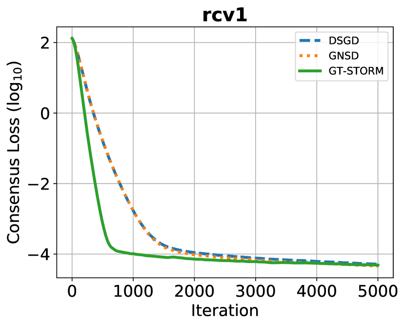
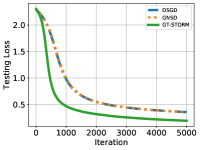
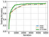
1-c) Results: We first compare the convergence rates of the algorithms. We adopt the consensus loss defined in the left-hand-side (LHS) of (3) as the criterion. After tuning, the best initial step-sizes are 0.1,0.1, 0.50.5 and 0.20.2 for a9aa9a, ijcnn1ijcnn1 and rcv1.binary,rcv1.binary, respectively. The results are shown in Figs. 44. It can be seen that our algorithm has a better performance: for a9aa9a and rcv1.binaryrcv1.binary datasets, all algorithms reach almost the same accuracy but our algorithm has a faster speed; for ijcnn1ijcnn1 dataset, our algorithm outperforms other methods both in the speed and accuracy.

Refer to caption
Figure 1. Non-convex logistic regression on LibSVM: a9a.
Refer to caption
Figure 2. Non-convex logistic regression on LibSVM: ijcnn1.
Refer to caption
Figure 3. Non-convex logistic regression on LibSVM: rcv1.
Refer to caption
Figure 4. Non-convex logistic regression: The effect of ρ\rho.
Refer to caption
Figure 5. Non-convex logistic regression: The effect of pcp_{c}.
Refer to caption
Figure 6. Non-convex logistic regression: The effect of mm.
Refer to caption
Figure 7. CNN experimental results on MNIST dataset.
Refer to caption
Figure 8. CNN experimental results on CIFAR-10 dataset.

Next, we examine the effect of the parameter ρ\rho on our algorithm. We focus on the a9aa9a dataset and fix the initial step-size as η0=0.1\eta_{0}\!=\!0.1. We choose ρ\rho from {101,100,101,102}.\{10^{-1},10^{0},10^{1},10^{2}\}. Note that ρ=102\rho=10^{2} is corresponding to the case ρ=1/η02.\rho\!=\!1/\eta_{0}^{2}. The results are shown in Fig. 4. It can be seen that the case ρ=101\rho\!=\!10^{1} has the best performance, which is followed by the case ρ=102.\rho=10^{2}. Also, as ρ\rho decreases, the convergence speed becomes slower (see the cases ρ=101\rho\!=\!10^{-1} and 10010^{0}).

In addition, we examine the effect of the network topology. We first fix the number of workers as m=10m=10 and change the the edge connectivity probability pcp_{c} from 0.350.35 to 0.9.0.9. Note that with a smaller pc,p_{c}, the network becomes sparser. We set η0=0.1\eta_{0}=0.1 and ρ=102.\rho=10^{2}. The results are shown in Fig. 8. Under different pcp_{c}-values, our algorithm has a similar performance in terms of convergence speed and accuracy. But with a larger pcp_{c}-values i.e., a denser network, the convergence speed slightly increases (see the zoom-in view in Fig. 8. Then, we fix the the edge connectivity probability pc=0.5p_{c}=0.5 but change the number of workers mm from 1010 to 50.50. We show the results in Fig. 8. It can be seen that with more workers, the algorithm converges faster and reaches a better accuracy.

2) Convolutional neural networks We use all three algorithms to train a convolutional neural network (CNN) model for image classification on MNIST and CIFAR-10 datasets. We adopt the same network topology as in the previous experiment. We use a non-identically distributed data partition strategy: the iith machine can access the data with the iith label. We fix the initial step-size as η0=0.01\eta_{0}=0.01 for all three algorithms and the remaining settings are the same as in the previous experiment.

2-a) Learning Models: For MNIST, the adopted CNN model has two convolutional layers (first of size 1×16×51\times 16\times 5 and then of size 16×32×516\times 32\times 5), each of which is followed by a max-pooling layer with size 2×22\times 2, and then a fully connected layer. The ReLU activation is used for the two convolutional layers and the “softmax” activation is applied at the output layer. The batch size is 64 for the CNN training on MNIST. For CIFAR-10, we apply the CNN model with two convolutional layers (first of size 3×6×53\times 6\times 5 and then of size 6×16×56\times 16\times 5). Each of the convolutional layers is followed by a max-pooling layer of size 2×22\times 2, and then three fully connected layers. The ReLU activation is used for the two convolutional layers and the first two fully connected layers, and the “softmax” activation is applied at the output layer. The batch size is chosen as 128 for the CNN training on CIFAR-10.

2-b) Results: Fig. 8 illustrates the testing accuracy of different algorithms versus iterations on MNIST and CIFAR-10 datasets. It can be seen from Fig. 8 that on the MNIST dataset, GNSD and GT-STORM have similar performance, but our GT-STORM maintains a faster speed and a better prediction accuracy. Compared with DSGD, our GT-STORM can gain about 10%10\% more accuracy. On the CIFAR-10 dataset (see Fig. 8), the performances of DSGD and GNSD deteriorate, while GT-STORM can achieve a better accuracy. Specifically, the accuracy of GT-STORM is around 15%15\% higher than that of GNSD and 25%25\% higher than that of DSGD.

5. Conclusion

In this paper, we proposed a gradient-tracking-based stochastic recursive momentum (GT-STORM) algorithm for decentralized non-convex optimization, which enjoys low sample, communication, and memory complexities. Our algorithm fuses the gradient tracking estimator and the variance reduction estimator and has a simple single-loop structure. Thus, it is more practical compared to existing works (e.g. GT-SAGA/SVRG and D-GET) in the literature. We have also conducted extensive numerical studies to verify the performance of our method, including non-convex logistic regression and neural networks. The numerical results show that our method outperforms the state-of-the-art methods when training on the large datasets. Our results in this work contribute to the increasingly important field of decentralized network training.

References

  • (1) B. Recht, C. Re, S. Wright, and F. Niu, “Hogwild: A lock-free approach to parallelizing stochastic gradient descent,” in Advances in neural information processing systems, 2011, pp. 693–701.
  • (2) M. Zinkevich, M. Weimer, L. Li, and A. J. Smola, “Parallelized stochastic gradient descent,” in Advances in neural information processing systems, 2010, pp. 2595–2603.
  • (3) J. Dean, G. Corrado, R. Monga, K. Chen, M. Devin, M. Mao, M. Ranzato, A. Senior, P. Tucker, K. Yang et al., “Large scale distributed deep networks,” in Advances in neural information processing systems, 2012, pp. 1223–1231.
  • (4) A. Nedic and A. Ozdaglar, “Distributed subgradient methods for multi-agent optimization,” IEEE Transactions on Automatic Control, vol. 54, no. 1, p. 48, 2009.
  • (5) X. Lian, C. Zhang, H. Zhang, C.-J. Hsieh, W. Zhang, and J. Liu, “Can decentralized algorithms outperform centralized algorithms? A case study for decentralized parallel stochastic gradient descent,” in Advances in Neural Information Processing Systems, 2017, pp. 5330–5340.
  • (6) J. Chen, Z. J. Towfic, and A. H. Sayed, “Dictionary learning over distributed models,” IEEE Transactions on Signal Processing, vol. 63, no. 4, pp. 1001–1016, 2014.
  • (7) Y. Cao, W. Yu, W. Ren, and G. Chen, “An overview of recent progress in the study of distributed multi-agent coordination,” IEEE Transactions on Industrial informatics, vol. 9, no. 1, pp. 427–438, 2012.
  • (8) K. Zhou and S. I. Roumeliotis, “Multirobot active target tracking with combinations of relative observations,” IEEE Transactions on Robotics, vol. 27, no. 4, pp. 678–695, 2011.
  • (9) W. Wang, J. Wang, M. Kolar, and N. Srebro, “Distributed stochastic multi-task learning with graph regularization,” arXiv preprint arXiv:1802.03830, 2018.
  • (10) X. Zhang, J. Liu, and Z. Zhu, “Distributed linear model clustering over networks: A tree-based fused-lasso admm approach,” arXiv preprint arXiv:1905.11549, 2019.
  • (11) K. Ali and W. Van Stam, “Tivo: Making show recommendations using a distributed collaborative filtering architecture,” in Proceedings of the tenth ACM SIGKDD international conference on Knowledge discovery and data mining, 2004, pp. 394–401.
  • (12) Z. Jiang, K. Mukherjee, and S. Sarkar, “On consensus-disagreement tradeoff in distributed optimization,” in 2018 Annual American Control Conference (ACC).   IEEE, 2018, pp. 571–576.
  • (13) J. N. Tsitsiklis, “Problems in decentralized decision making and computation.” Massachusetts Inst of Tech Cambridge Lab for Information and Decision Systems, Tech. Rep., 1984.
  • (14) Q. Tran-Dinh, N. H. Pham, D. T. Phan, and L. M. Nguyen, “Hybrid stochastic gradient descent algorithms for stochastic nonconvex optimization,” arXiv preprint arXiv:1905.05920, 2019.
  • (15) A. Cutkosky and F. Orabona, “Momentum-based variance reduction in non-convex sgd,” in Advances in Neural Information Processing Systems, 2019, pp. 15 210–15 219.
  • (16) P. Di Lorenzo and G. Scutari, “Next: In-network nonconvex optimization,” IEEE Transactions on Signal and Information Processing over Networks, vol. 2, no. 2, pp. 120–136, 2016.
  • (17) S. Lu, X. Zhang, H. Sun, and M. Hong, “GNSD: a gradient-tracking based nonconvex stochastic algorithm for decentralized optimization,” in 2019 IEEE Data Science Workshop, DSW 2019.   Institute of Electrical and Electronics Engineers Inc., 2019, pp. 315–321.
  • (18) Z. Jiang, A. Balu, C. Hegde, and S. Sarkar, “Collaborative deep learning in fixed topology networks,” in Advances in Neural Information Processing Systems, 2017, pp. 5904–5914.
  • (19) H. Sun, S. Lu, and M. Hong, “Improving the sample and communication complexity for decentralized non-convex optimization: A joint gradient estimation and tracking approach,” ICML 2020, 2019.
  • (20) S. Ghadimi and G. Lan, “Stochastic first-and zeroth-order methods for nonconvex stochastic programming,” SIAM Journal on Optimization, vol. 23, no. 4, pp. 2341–2368, 2013.
  • (21) L. Bottou, F. E. Curtis, and J. Nocedal, “Optimization methods for large-scale machine learning,” Siam Review, vol. 60, no. 2, pp. 223–311, 2018.
  • (22) P. Zhou, X. Yuan, and J. Feng, “New insight into hybrid stochastic gradient descent: Beyond with-replacement sampling and convexity,” in Advances in Neural Information Processing Systems, 2018, pp. 1234–1243.
  • (23) R. Johnson and T. Zhang, “Accelerating stochastic gradient descent using predictive variance reduction,” in Advances in neural information processing systems, 2013, pp. 315–323.
  • (24) S. J. Reddi, A. Hefny, S. Sra, B. Póczos, and A. Smola, “Stochastic variance reduction for nonconvex optimization,” in International conference on machine learning, 2016, pp. 314–323.
  • (25) A. Defazio, F. Bach, and S. Lacoste-Julien, “Saga: A fast incremental gradient method with support for non-strongly convex composite objectives,” in Advances in neural information processing systems, 2014, pp. 1646–1654.
  • (26) L. Lei, C. Ju, J. Chen, and M. I. Jordan, “Non-convex finite-sum optimization via scsg methods,” in Advances in Neural Information Processing Systems, 2017, pp. 2348–2358.
  • (27) C. Fang, C. J. Li, Z. Lin, and T. Zhang, “Spider: Near-optimal non-convex optimization via stochastic path-integrated differential estimator,” in Advances in Neural Information Processing Systems, 2018, pp. 689–699.
  • (28) L. M. Nguyen, J. Liu, K. Scheinberg, and M. Takác, “Sarah: A novel method for machine learning problems using stochastic recursive gradient,” in Proceedings of the 34th International Conference on Machine Learning-Volume 70.   JMLR. org, 2017, pp. 2613–2621.
  • (29) Z. Wang, K. Ji, Y. Zhou, Y. Liang, and V. Tarokh, “Spiderboost and momentum: Faster variance reduction algorithms,” in Advances in Neural Information Processing Systems, 2019, pp. 2403–2413.
  • (30) K. Yuan, Q. Ling, and W. Yin, “On the convergence of decentralized gradient descent,” SIAM Journal on Optimization, vol. 26, no. 3, pp. 1835–1854, 2016.
  • (31) W. Shi, Q. Ling, G. Wu, and W. Yin, “Extra: An exact first-order algorithm for decentralized consensus optimization,” SIAM Journal on Optimization, vol. 25, no. 2, pp. 944–966, 2015.
  • (32) H. Sun and M. Hong, “Distributed non-convex first-order optimization and information processing: Lower complexity bounds and rate optimal algorithms,” IEEE Transactions on Signal processing, vol. 67, no. 22, pp. 5912–5928, 2019.
  • (33) J. F. Mota, J. M. Xavier, P. M. Aguiar, and M. Püschel, “D-admm: A communication-efficient distributed algorithm for separable optimization,” IEEE Transactions on Signal Processing, vol. 61, no. 10, pp. 2718–2723, 2013.
  • (34) A. Mokhtari, W. Shi, Q. Ling, and A. Ribeiro, “A decentralized second-order method with exact linear convergence rate for consensus optimization,” IEEE Transactions on Signal and Information Processing over Networks, vol. 2, no. 4, pp. 507–522, 2016.
  • (35) M. Eisen, A. Mokhtari, and A. Ribeiro, “Decentralized quasi-newton methods,” IEEE Transactions on Signal Processing, vol. 65, no. 10, pp. 2613–2628, 2017.
  • (36) A. Nedić, A. Olshevsky, and M. G. Rabbat, “Network topology and communication-computation tradeoffs in decentralized optimization,” Proceedings of the IEEE, vol. 106, no. 5, pp. 953–976, 2018.
  • (37) T.-H. Chang, M. Hong, H.-T. Wai, X. Zhang, and S. Lu, “Distributed learning in the non-convex world: From batch to streaming data, and beyond,” arXiv preprint arXiv:2001.04786, 2020.
  • (38) J. Zeng and W. Yin, “On nonconvex decentralized gradient descent,” IEEE Transactions on signal processing, vol. 66, no. 11, pp. 2834–2848, 2018.
  • (39) A. Mokhtari and A. Ribeiro, “DSA: decentralized double stochastic averaging gradient algorithm,” The Journal of Machine Learning Research, vol. 17, no. 1, pp. 2165–2199, 2016.
  • (40) K. Yuan, B. Ying, J. Liu, and A. H. Sayed, “Variance-reduced stochastic learning by networked agents under random reshuffling,” IEEE Transactions on Signal Processing, vol. 67, no. 2, pp. 351–366, 2018.
  • (41) R. Xin, U. A. Khan, and S. Kar, “Variance-reduced decentralized stochastic optimization with gradient tracking,” arXiv preprint arXiv:1909.11774, 2019.
  • (42) A. Nedich, A. Olshevsky, and W. Shi, “A geometrically convergent method for distributed optimization over time-varying graphs,” in 2016 IEEE 55th Conference on Decision and Control (CDC).   IEEE, 2016, pp. 1023–1029.
  • (43) Y. Zhou, Y. Liang, and H. Zhang, “Generalization error bounds with probabilistic guarantee for sgd in nonconvex optimization,” arXiv preprint arXiv:1802.06903, 2018.
  • (44) S. P. Karimireddy, Q. Rebjock, S. U. Stich, and M. Jaggi, “Error feedback fixes SignSGD and other gradient compression schemes,” arXiv preprint arXiv:1901.09847, 2019.
  • (45) A. Koloskova, S. U. Stich, and M. Jaggi, “Decentralized stochastic optimization and gossip algorithms with compressed communication,” arXiv preprint arXiv:1902.00340, 2019.
  • (46) Z. Wang, Y. Zhou, Y. Liang, and G. Lan, “Cubic regularization with momentum for nonconvex optimization,” arXiv preprint arXiv:1810.03763, 2018.
  • (47) X. Zhang, J. Liu, Z. Zhu, and E. S. Bentley. (2020) GT-STORM: taming sample, communication, and memory complexities in decentralized non-convex learning. [Online]. Available: https://kevinliu-osu-ece.github.io/publications/GT-STORM_TR.pdf

Appendix A Addtional Experiment Details

Refer to caption
Figure 9. The network topology generated by the Erdo¨\ddot{\text{o}}s-Re`\grave{\text{e}}nyi graph.

In our simulation, the communication graph 𝒢\mathcal{G} is generated by the Erdo¨\ddot{\text{o}}s-Re`\grave{\text{e}}nyi graph with different edge connectivity probability pcp_{c} and nodes number mm. We set m=10m=10 and pc=0.5p_{c}=0.5. The generated graph is shown in Figure 9.

A.1. Nonconvex Logistic Regression

In Section 4.1, we set the step-size as ηt=η0/1+0.1×t\eta_{t}=\eta_{0}/\sqrt{1+0.1\times t} for DSGD and GNSD, while ηt=η0/1+0.1×t3\eta_{t}=\eta_{0}/\sqrt[3]{1+0.1\times t} for GT-STORM. It can be noted that the step-size adopted for GT-STORM is diminishing slower than those for DSGD and GNSD, though the choices are following the theoretical results. Thus, here we apply the step-size as ηt=η0/1+0.1×t3\eta_{t}=\eta_{0}/\sqrt[3]{1+0.1\times t} for all the three algorithms. We tune the initial step-size η0\eta_{0} by searching the grid {0.01,0.02,0.05,0.1,0.2,0.5,1.0}.\{0.01,0.02,0.05,0.1,0.2,0.5,1.0\}. After tuning, the best initial step-sizes are 0.1,0.1, 0.50.5 and 0.20.2 for a9aa9a, ijcnn1ijcnn1 and rcv1.binary,rcv1.binary, respectively. We show the results in Figure 10. It can be seen that with a larger step-size, though the convergence is faster for DSGD and GNSD at the beginning, the accuracy is unsatisfactory (e.g. a9aa9a and rcv1.binaryrcv1.binary). Also, with the same step-size, our algorithm performs much better than the other two.

Refer to caption
Refer to caption
Refer to caption
Figure 10. Experimental results for nonconvex logistic regression on LibSVM datasets: the three algorithms adopt a diminishing step-size ηt=η0/1+0.1×t3;\eta_{t}=\eta_{0}/\sqrt[3]{1+0.1\times t}; the curves are averaged over 10 random trials and the shaded regions represent the standard deviation.

A.2. Convolutional Neural Networks

Here we show the testing loss and accuracy for the CNN models on the MNIST and CIFAR-10 datasets in Figure 11-12. In all experiment results, our algorithm has a better performance: a higher accuracy and a smaller loss. The final testing accuracy results are summarized in Table 1.

Refer to caption Refer to caption Refer to caption Refer to caption
(a) I.D. data partition (b) N.D. data partition
Figure 11. Experimental results for CNN on MNIST dataset.
Refer to caption Refer to caption Refer to caption Refer to caption
(a) I.D. data partition (b) N.D. data partition
Figure 12. Experimental results for CNN on CIFAR-10 dataset.
Table 1. The results of testing accuracy with the CNN models trained by different algorithms.
Dataset DSGD GNSD GT-STORM
MNIST I.D. 0.9102 0.9102 0.9375
N.D. 0.8203 0.9102 0.9257
CIFAR-10 I.D. 0.6093 0.6016 0.7734
N.D. 0.5352 0.6133 0.7695

Appendix B Proof of Main Results

Due to space limitation, we provide key proof steps of the key lemmas and theorems in this appendix. We refer readers to (Zhang20:GT-STORM_TR, ) for the complete proofs.

B.1. Proof for Lemma 1

Proof.

Recall that 𝐯¯t=βt(𝐯¯t1+𝐰¯t)+(1βt)𝐮¯t\bar{\mathbf{v}}_{t}=\beta_{t}(\bar{\mathbf{v}}_{t-1}+\bar{\mathbf{w}}_{t})+(1-\beta_{t})\bar{\mathbf{u}}_{t}, then

𝐯¯t𝐠¯t2=βt(𝐯¯t1+𝐰¯t)+(1βt)𝐮¯t𝐠¯t2\displaystyle\|\bar{\mathbf{v}}_{t}\!-\!\bar{\mathbf{g}}_{t}\|^{2}=\|\beta_{t}(\bar{\mathbf{v}}_{t\!-\!1}+\bar{\mathbf{w}}_{t})\!+\!(1\!-\!\beta_{t})\bar{\mathbf{u}}_{t}\!-\!\bar{\mathbf{g}}_{t}\|^{2}
=\displaystyle= βt(𝐯¯t1𝐠¯t1)+βt(𝐰¯t𝐠¯t+𝐠¯t1)+(1βt)(𝐮¯t𝐠¯t)2\displaystyle\|\beta_{t}(\bar{\mathbf{v}}_{t\!-\!1}\!-\!\bar{\mathbf{g}}_{t\!-\!1})\!+\!\beta_{t}(\bar{\mathbf{w}}_{t}\!-\!\bar{\mathbf{g}}_{t}\!+\!\bar{\mathbf{g}}_{t\!-\!1})\!+\!(1\!-\!\beta_{t})(\bar{\mathbf{u}}_{t}\!-\!\bar{\mathbf{g}}_{t})\|^{2}
=\displaystyle= βt2𝐯¯t1𝐠¯t12+βt(𝐰¯t𝐠¯t+𝐠¯t1)+(1βt)(𝐮¯t𝐠¯t)2\displaystyle\beta_{t}^{2}\|\bar{\mathbf{v}}_{t\!-\!1}\!-\!\bar{\mathbf{g}}_{t\!-\!1}\|^{2}\!+\!\|\beta_{t}(\bar{\mathbf{w}}_{t}\!-\!\bar{\mathbf{g}}_{t}\!+\!\bar{\mathbf{g}}_{t\!-\!1})\!+\!(1\!-\!\beta_{t})(\bar{\mathbf{u}}_{t}\!-\!\bar{\mathbf{g}}_{t})\|^{2}
(21) +2𝐯¯t1𝐠¯t1,βt(𝐰¯t𝐠¯t+𝐠¯t1)+(1βt)(𝐮¯t𝐠¯t)\displaystyle\!+\!2\langle\bar{\mathbf{v}}_{t\!-\!1}\!-\!\bar{\mathbf{g}}_{t\!-\!1},\beta_{t}(\bar{\mathbf{w}}_{t}\!-\!\bar{\mathbf{g}}_{t}\!+\!\bar{\mathbf{g}}_{t\!-\!1})\!+\!(1\!-\!\beta_{t})(\bar{\mathbf{u}}_{t}\!-\!\bar{\mathbf{g}}_{t})\rangle

Note that 𝔼ζt[𝐰¯t]=𝐠¯t𝐠¯t1\mathbb{E}_{\zeta_{t}}[\bar{\mathbf{w}}_{t}]=\bar{\mathbf{g}}_{t}-\bar{\mathbf{g}}_{t-1} and 𝔼ζt[𝐮¯t]=𝐠¯t.\mathbb{E}_{\zeta_{t}}[\bar{\mathbf{u}}_{t}]=\bar{\mathbf{g}}_{t}. Taking expectation with respect to ζt,\zeta_{t}, we have:

𝔼ζt[𝐯¯t𝐠¯t2]\displaystyle\mathbb{E}_{\zeta_{t}}[\|\bar{\mathbf{v}}_{t}-\bar{\mathbf{g}}_{t}\|^{2}]
=(a)βt2𝐯¯t1𝐠¯t12+𝔼ζt[βt(𝐰¯t𝐠¯t+𝐠¯t1)+(1βt)(𝐮¯t𝐠¯t)2]\displaystyle\stackrel{{\scriptstyle(a)}}{{=}}\beta_{t}^{2}\|\bar{\mathbf{v}}_{t\!-\!1}\!-\!\bar{\mathbf{g}}_{t\!-\!1}\|^{2}\!+\!\mathbb{E}_{\zeta_{t}}[\|\beta_{t}(\bar{\mathbf{w}}_{t}\!-\!\bar{\mathbf{g}}_{t}\!+\!\bar{\mathbf{g}}_{t\!-\!1})\!+\!(1\!-\!\beta_{t})(\bar{\mathbf{u}}_{t}\!-\!\bar{\mathbf{g}}_{t})\|^{2}]
(b)βt2𝐯¯t1𝐠¯t12+𝔼ζt[2βt2𝐰¯t𝐠¯t+𝐠¯t12+2(1βt)2𝐮¯t𝐠¯t2]\displaystyle\stackrel{{\scriptstyle(b)}}{{\leq}}\beta_{t}^{2}\|\bar{\mathbf{v}}_{t\!-\!1}\!-\!\bar{\mathbf{g}}_{t-1}\|^{2}\!\!\!+\!\mathbb{E}_{\zeta_{t}}\![2\beta_{t}^{2}\|\bar{\mathbf{w}}_{t}\!-\!\bar{\mathbf{g}}_{t}\!\!+\!\bar{\mathbf{g}}_{t\!-\!1}\|^{2}\!\!\!+\!2(1\!-\!\beta_{t})^{2}\|\bar{\mathbf{u}}_{t}\!-\!\bar{\mathbf{g}}_{t}\|^{2}\!]
(c)βt2𝐯¯t1𝐠¯t12+2βt2𝔼ζt[𝐰¯t2]+2(1βt)2σ2m\displaystyle\stackrel{{\scriptstyle(c)}}{{\leq}}\beta_{t}^{2}\|\bar{\mathbf{v}}_{t\!-\!1}-\bar{\mathbf{g}}_{t\!-\!1}\|^{2}+2\beta_{t}^{2}\mathbb{E}_{\zeta_{t}}[\|\bar{\mathbf{w}}_{t}\|^{2}]+\frac{2(1-\beta_{t})^{2}\sigma^{2}}{m}
(d)βt2𝐯¯t1𝐠¯t12+2βt2mi=1m𝔼ζt[𝐰i,t2]+2(1βt)2σ2m\displaystyle\stackrel{{\scriptstyle(d)}}{{\leq}}\beta_{t}^{2}\|\bar{\mathbf{v}}_{t\!-\!1}\!-\!\bar{\mathbf{g}}_{t\!-\!1}\|^{2}\!+\!\frac{2\beta_{t}^{2}}{m}\sum_{i=1}^{m}\mathbb{E}_{\zeta_{t}}[\|\mathbf{w}_{i,t}\|^{2}]+\frac{2(1-\beta_{t})^{2}\sigma^{2}}{m}
(e)βt2𝐯¯t1𝐠¯t12+2βt2L2mi=1m𝔼ζt[𝐱i,t𝐱i,t12]+2(1βt)2σ2m\displaystyle\stackrel{{\scriptstyle(e)}}{{\leq}}\beta_{t}^{2}\|\bar{\mathbf{v}}_{t\!-\!1}\!-\!\bar{\mathbf{g}}_{t\!-\!1}\|^{2}\!\!+\!\frac{2\beta_{t}^{2}L^{2}}{m}\sum_{i=1}^{m}\mathbb{E}_{\zeta_{t}}[\|\mathbf{x}_{i,t}\!-\!\mathbf{x}_{i,t\!-\!1}\|^{2}]\!+\!\frac{2(1\!-\!\beta_{t})^{2}\sigma^{2}}{m}
(22) =βt2𝐯¯t1𝐠¯t12+2βt2L2m𝔼ζt[𝐱t𝐱t12]+2(1βt)2σ2m,\displaystyle=\beta_{t}^{2}\|\bar{\mathbf{v}}_{t\!-\!1}\!-\!\bar{\mathbf{g}}_{t\!-\!1}\|^{2}\!+\!\frac{2\beta_{t}^{2}L^{2}}{m}\mathbb{E}_{\zeta_{t}}[\|\mathbf{x}_{t}\!-\!\mathbf{x}_{t\!-\!1}\|^{2}]\!+\!\frac{2(1\!-\!\beta_{t})^{2}\sigma^{2}}{m},

where (a) is because the cross term has the expectation as zero; (b) is by 𝐚+𝐛22𝐚2+2𝐛2;\|\mathbf{a}+\mathbf{b}\|^{2}\leq 2\|\mathbf{a}\|^{2}+2\|\mathbf{b}\|^{2}; (c) is by 𝔼[𝐗𝔼[𝐗]2]𝔼[𝐗2]\mathbb{E}[\|\mathbf{X}-\mathbb{E}[\mathbf{X}]\|^{2}]\leq\mathbb{E}[\|\mathbf{X}\|^{2}] and Assumption 1 (c); (d) is because of the Jensen’s inequality; (e) is by the LL-average smoothness. Thus, taking the full expectation, it holds that

𝔼[𝐯¯t𝐠¯t2]\displaystyle\mathbb{E}[\|\bar{\mathbf{v}}_{t}-\bar{\mathbf{g}}_{t}\|^{2}]\leq βt2𝔼[𝐯¯t1𝐠¯t12]\displaystyle\beta_{t}^{2}\mathbb{E}[\|\bar{\mathbf{v}}_{t-1}-\bar{\mathbf{g}}_{t-1}\|^{2}]
(23) +2βt2L2m𝔼[𝐱t𝐱t12]+2(1βt)2σ2m.\displaystyle+\frac{2\beta_{t}^{2}L^{2}}{m}\mathbb{E}[\|\mathbf{x}_{t}-\mathbf{x}_{t-1}\|^{2}]+\frac{2(1-\beta_{t})^{2}\sigma^{2}}{m}.

B.2. Proof for Lemma 2

Proof.

From the LL-smoothness of f,f, we have:

f(𝐱¯t+1)f(𝐱¯t)ηtf(𝐱¯t),𝐯¯t+Lηt22𝐯¯t2\displaystyle f(\mathbf{\bar{x}}_{t\!+\!1})\!\leq\!f(\mathbf{\bar{x}}_{t})\!-\!\eta_{t}\langle\nabla f(\mathbf{\bar{x}}_{t}),\bar{\mathbf{v}}_{t}\rangle\!+\!\frac{L\eta_{t}^{2}}{2}\|\bar{\mathbf{v}}_{t}\|^{2}
=f(𝐱¯t)ηt2f(𝐱¯t)2(ηt2Lηt22)𝐯¯t2+ηt2𝐯¯tf(𝐱¯t)2\displaystyle\!=\!f(\mathbf{\bar{x}}_{t})\!-\!\frac{\eta_{t}}{2}\|\nabla\!f(\mathbf{\bar{x}}_{t})\|^{2}\!-\!(\frac{\eta_{t}}{2}\!-\!\frac{L\eta_{t}^{2}}{2})\|\bar{\mathbf{v}}_{t}\|^{2}\!+\!\frac{\eta_{t}}{2}\!\|\bar{\mathbf{v}}_{t}\!-\!\nabla\!f(\mathbf{\bar{x}}_{t})\|^{2}
f(𝐱¯t)ηt2f(𝐱¯t)2(ηt2Lηt22)𝐯¯t2\displaystyle\!\leq\!f(\mathbf{\bar{x}}_{t})\!-\!\frac{\eta_{t}}{2}\!\|\nabla f(\mathbf{\bar{x}}_{t})\|^{2}\!-\!(\frac{\eta_{t}}{2}\!-\!\frac{L\eta_{t}^{2}}{2})\|\bar{\mathbf{v}}_{t}\|^{2}
+ηt𝐯¯t𝐠¯t2+ηt𝐠¯tf(𝐱¯t)2\displaystyle+\!\eta_{t}\|\bar{\mathbf{v}}_{t}\!-\!\bar{\mathbf{g}}_{t}\|^{2}\!+\!\eta_{t}\|\bar{\mathbf{g}}_{t}\!-\!\nabla f(\mathbf{\bar{x}}_{t})\|^{2}
(a)f(𝐱¯t)ηt2f(𝐱¯t)2(ηt2Lηt22)𝐯¯t2\displaystyle\stackrel{{\scriptstyle(a)}}{{\leq}}f(\mathbf{\bar{x}}_{t})\!-\!\frac{\eta_{t}}{2}\|\nabla f(\mathbf{\bar{x}}_{t})\|^{2}\!-\!(\frac{\eta_{t}}{2}\!-\!\frac{L\eta_{t}^{2}}{2})\|\bar{\mathbf{v}}_{t}\|^{2}
+ηt𝐯¯t𝐠¯t2+ηtmi=1m𝐠i,tfi(𝐱¯t)2\displaystyle+\!\eta_{t}\|\bar{\mathbf{v}}_{t}\!-\!\bar{\mathbf{g}}_{t}\|^{2}\!+\!\frac{\eta_{t}}{m}\sum_{i=1}^{m}\|\mathbf{g}_{i,t}\!-\!\nabla f_{i}(\mathbf{\bar{x}}_{t})\|^{2}
(b)f(𝐱¯t)ηt2f(𝐱¯t)2(ηt2Lηt22)𝐯¯t2\displaystyle\stackrel{{\scriptstyle(b)}}{{\leq}}f(\mathbf{\bar{x}}_{t})\!-\!\frac{\eta_{t}}{2}\|\nabla f(\mathbf{\bar{x}}_{t})\|^{2}\!-\!(\frac{\eta_{t}}{2}\!-\!\frac{L\eta_{t}^{2}}{2})\|\bar{\mathbf{v}}_{t}\|^{2}
(24) +ηt𝐯¯t𝐠¯t2+L2ηtm𝐱t𝟏𝐱¯t2,\displaystyle+\!\eta_{t}\|\bar{\mathbf{v}}_{t}\!-\!\bar{\mathbf{g}}_{t}\|^{2}\!+\!\frac{L^{2}\eta_{t}}{m}\|\mathbf{x}_{t}\!-\!\mathbf{1}\otimes\mathbf{\bar{x}}_{t}\|^{2},

where 𝐠¯t=1mi=1m𝐠i,t\bar{\mathbf{g}}_{t}=\frac{1}{m}\sum_{i=1}^{m}\mathbf{g}_{i,t} and 𝐠i,t=fi(𝐱i,t),\mathbf{g}_{i,t}=\nabla f_{i}(\mathbf{x}_{i,t}), (a) is because of the Jensen’s inequality and (b) is by the LL-average smoothness. Take the full expectation on the above inequality:

𝔼[f(𝐱¯t+1)]𝔼[f(\displaystyle\mathbb{E}[f(\mathbf{\bar{x}}_{t\!+\!1})]\!-\!\mathbb{E}[f( 𝐱¯t)]ηt2𝔼[f(𝐱¯t)2](ηt2Lηt22)𝔼[𝐯¯t2]\displaystyle\mathbf{\bar{x}}_{t})]\!\leq\!-\!\frac{\eta_{t}}{2}\mathbb{E}[\|\nabla f(\mathbf{\bar{x}}_{t})\|^{2}]\!-\!(\frac{\eta_{t}}{2}\!-\!\frac{L\eta_{t}^{2}}{2})\mathbb{E}[\|\bar{\mathbf{v}}_{t}\|^{2}]
(25) +ηt𝔼[𝐯¯t𝐠¯t2]+L2ηtm𝔼[𝐱t𝟏𝐱¯t2].\displaystyle\!+\!\eta_{t}\mathbb{E}[\|\bar{\mathbf{v}}_{t}\!-\!\bar{\mathbf{g}}_{t}\|^{2}]\!+\!\frac{L^{2}\eta_{t}}{m}\mathbb{E}[\|\mathbf{x}_{t}\!-\!\mathbf{1}\!\otimes\!\mathbf{\bar{x}}_{t}\|^{2}].

B.3. Proof for Lemma 3

Proof.

First for the iterate 𝐱t,\mathbf{x}_{t}, we have the following contraction:

(26) 𝐖~𝐱t𝟏𝐱¯t2=𝐖~(𝐱t𝟏𝐱¯t)2λ2𝐱t𝟏𝐱¯t2,\displaystyle\|\tilde{\mathbf{W}}\mathbf{x}_{t}\!-\!\mathbf{1}\otimes\mathbf{\bar{x}}_{t}\|^{2}\!=\!\|\tilde{\mathbf{W}}(\mathbf{x}_{t}\!-\!\mathbf{1}\!\otimes\!\mathbf{\bar{x}}_{t})\|^{2}\!\leq\!\lambda^{2}\|\mathbf{x}_{t}\!-\!\mathbf{1}\!\otimes\!\mathbf{\bar{x}}_{t}\|^{2},

This is because 𝐱t𝟏𝐱¯t\mathbf{x}_{t}-\mathbf{1}\otimes\mathbf{\bar{x}}_{t} is orthogonal to 𝟏,\mathbf{1}, which is the eigenvector corresponding to the largest eigenvalue of 𝐖~,\tilde{\mathbf{W}}, and λ=max{|λ2|,|λm|}.\lambda=\max\{|\lambda_{2}|,|\lambda_{m}|\}. Recall that 𝐱¯t+1=𝐱¯tηt𝐯¯t,\mathbf{\bar{x}}_{t+1}=\mathbf{\bar{x}}_{t}-\eta_{t}\bar{\mathbf{v}}_{t}, hence,

𝐱t+1𝟏𝐱¯t+12=𝐖~𝐱tηt𝐯t𝟏(𝐱¯tηt𝐯¯t)2\displaystyle\|\mathbf{x}_{t+1}-\mathbf{1}\otimes\mathbf{\bar{x}}_{t+1}\|^{2}=\|\tilde{\mathbf{W}}\mathbf{x}_{t}-\eta_{t}\mathbf{v}_{t}-\mathbf{1}\otimes(\mathbf{\bar{x}}_{t}-\eta_{t}\bar{\mathbf{v}}_{t})\|^{2}
(1+c1)𝐖~𝐱t𝟏𝐱¯t2+(1+1c1)ηt2𝐯t𝟏𝐯¯t2\displaystyle\leq(1+c_{1})\|\tilde{\mathbf{W}}\mathbf{x}_{t}-\mathbf{1}\otimes\mathbf{\bar{x}}_{t}\|^{2}+(1+\frac{1}{c_{1}})\eta_{t}^{2}\|\mathbf{v}_{t}-\mathbf{1}\otimes\bar{\mathbf{v}}_{t}\|^{2}
(27) (1+c1)λ2𝐱t𝟏𝐱¯t2+(1+1c1)ηt2𝐯t𝟏𝐯¯t2.\displaystyle\leq(1+c_{1})\lambda^{2}\|\mathbf{x}_{t}-\mathbf{1}\otimes\mathbf{\bar{x}}_{t}\|^{2}+(1+\frac{1}{c_{1}})\eta_{t}^{2}\|\mathbf{v}_{t}-\mathbf{1}\otimes\bar{\mathbf{v}}_{t}\|^{2}.

Similarly to (B.3), we have:

𝐯t+1𝟏𝐯¯t+12\displaystyle\|\mathbf{v}_{t\!+\!1}\!-\!\mathbf{1}\!\otimes\!\bar{\mathbf{v}}_{t\!+\!1}\|^{2}
=\displaystyle\!= βt+1(𝐖~𝐯t+𝐰t+1)+(1βt)𝐮t+1𝟏(βt+1(𝐯¯t\displaystyle\|\beta_{t\!+\!1}(\tilde{\mathbf{W}}\mathbf{v}_{t}\!+\!\mathbf{w}_{t\!+\!1})\!+\!(1\!-\!\beta_{t})\mathbf{u}_{t\!+\!1}\!-\!\mathbf{1}\!\otimes\!\big{(}\beta_{t\!+\!1}(\bar{\mathbf{v}}_{t}
+𝐰¯t+1)+(1βt+1)𝐮¯t+1)\displaystyle+\!\bar{\mathbf{w}}_{t\!+\!1})\!+\!(1\!-\!\beta_{t\!+\!1})\bar{\mathbf{u}}_{t\!+\!1}\big{)}\|
\displaystyle\!\leq (1+c1)βt+12λ2𝐯t𝟏𝐯¯t2+(1+1c1)βt+1(𝐰t+1\displaystyle(1\!+\!c_{1})\beta_{t\!+\!1}^{2}\lambda^{2}\|\mathbf{v}_{t}\!-\!\mathbf{1}\!\otimes\!\bar{\mathbf{v}}_{t}\|^{2}\!+\!(1\!+\!\frac{1}{c_{1}})\|\beta_{t\!+\!1}(\mathbf{w}_{t\!+\!1}
𝟏𝐰¯t+1)+(1βt+1)(𝐮t+1𝟏𝐮¯t+1)2\displaystyle\!-\!\mathbf{1}\!\otimes\!\bar{\mathbf{w}}_{t\!+\!1})\!+\!(1\!-\!\beta_{t\!+\!1})(\mathbf{u}_{t\!+\!1}\!-\!\mathbf{1}\!\otimes\!\bar{\mathbf{u}}_{t\!+\!1})\|^{2}
\displaystyle\!\leq (1+c1)βt+12λ2𝐯t𝟏𝐯¯t2+2(1+1c1)(βt+12𝐰t+1\displaystyle(1\!+\!c_{1})\beta_{t\!+\!1}^{2}\lambda^{2}\|\mathbf{v}_{t}\!-\!\mathbf{1}\!\otimes\!\bar{\mathbf{v}}_{t}\|^{2}\!+\!2(1\!+\!\frac{1}{c_{1}})\big{(}\beta_{t\!+\!1}^{2}\|\mathbf{w}_{t\!+\!1}
𝟏𝐰¯t+12+(1βt+1)2𝐮t+1𝟏𝐮¯t+12)\displaystyle\!-\!\mathbf{1}\!\otimes\!\bar{\mathbf{w}}_{t\!+\!1}\|^{2}\!+\!(1\!-\!\beta_{t\!+\!1})^{2}\|\mathbf{u}_{t\!+\!1}\!-\!\mathbf{1}\!\otimes\!\bar{\mathbf{u}}_{t\!+\!1}\|^{2}\big{)}
(a)\displaystyle\!\stackrel{{\scriptstyle(a)}}{{\leq}}\! (1+c1)βt+12λ2𝐯t𝟏𝐯¯t2\displaystyle(1\!+\!c_{1})\beta_{t\!+\!1}^{2}\lambda^{2}\|\mathbf{v}_{t}\!-\!\mathbf{1}\!\otimes\!\bar{\mathbf{v}}_{t}\|^{2}
(28) +2(1+1c1)(βt+12𝐰t+12+(1βt+1)2𝐮t+12)\displaystyle\!+\!2(1\!+\!\frac{1}{c_{1}})\big{(}\beta_{t\!+\!1}^{2}\|\mathbf{w}_{t\!+\!1}\|^{2}\!+\!(1\!-\!\beta_{t\!+\!1})^{2}\|\mathbf{u}_{t\!+\!1}\|^{2}\big{)}

where (a) is due to 𝐈1m𝟏𝟏1.\|\mathbf{I}-\frac{1}{m}\mathbf{1}\mathbf{1}^{\top}\|\leq 1. Lastly, according to the updating equation (9) in main paper, it holds

𝐱t+1𝐱t2=𝐖~𝐱tηt𝐯t𝐱t2\displaystyle\|\mathbf{x}_{t+1}-\mathbf{x}_{t}\|^{2}=\|\tilde{\mathbf{W}}\mathbf{x}_{t}-\eta_{t}\mathbf{v}_{t}-\mathbf{x}_{t}\|^{2}
=\displaystyle= (𝐖~𝐈)𝐱tηt𝐯t22(𝐖~𝐈)𝐱t2+2ηt2𝐯t2\displaystyle\|(\tilde{\mathbf{W}}-\mathbf{I})\mathbf{x}_{t}-\eta_{t}\mathbf{v}_{t}\|^{2}\leq 2\|(\tilde{\mathbf{W}}-\mathbf{I})\mathbf{x}_{t}\|^{2}+2\eta_{t}^{2}\|\mathbf{v}_{t}\|^{2}
=\displaystyle= 2(𝐖~𝐈)(𝐱t𝟏𝐱¯t)2+2ηt2𝐯t2\displaystyle 2\|(\tilde{\mathbf{W}}-\mathbf{I})(\mathbf{x}_{t}-\mathbf{1}\otimes\mathbf{\bar{x}}_{t})\|^{2}+2\eta_{t}^{2}\|\mathbf{v}_{t}\|^{2}
(29) (a)\displaystyle\stackrel{{\scriptstyle(a)}}{{\leq}} 8(𝐱t𝟏𝐱¯t)2+4ηt2𝐯t𝟏𝐯¯t2+4ηt2m𝐯¯t2,\displaystyle 8\|(\mathbf{x}_{t}-\mathbf{1}\otimes\mathbf{\bar{x}}_{t})\|^{2}+4\eta_{t}^{2}\|\mathbf{v}_{t}-\mathbf{1}\otimes\bar{\mathbf{v}}_{t}\|^{2}+4\eta_{t}^{2}m\|\bar{\mathbf{v}}_{t}\|^{2},

where (a) is because 𝐖~𝐈2.\|\tilde{\mathbf{W}}-\mathbf{I}\|\leq 2.

B.4. Proof for Lemma 4

Proof.

First, with ηt=τ/(ω+t)1/3,\eta_{t}=\tau/(\omega+t)^{1/3}, we have:

1ηt1ηt1\displaystyle\frac{1}{\eta_{t}}-\frac{1}{\eta_{t-1}} =1τ((ω+t)13(ω+t1)13)\displaystyle=\frac{1}{\tau}\big{(}(\omega+t)^{\frac{1}{3}}-(\omega+t-1)^{\frac{1}{3}}\big{)}
(a)13τ1(ω+t1)23=13τ3ηt12\displaystyle\stackrel{{\scriptstyle(a)}}{{\leq}}\frac{1}{3\tau}\cdot\frac{1}{(\omega+t-1)^{\frac{2}{3}}}=\frac{1}{3\tau^{3}}\eta_{t-1}^{2}
(b)13τ1(ω2+t)2313τ223(ω+t)23\displaystyle\stackrel{{\scriptstyle(b)}}{{\leq}}\frac{1}{3\tau}\cdot\frac{1}{(\frac{\omega}{2}+t)^{\frac{2}{3}}}\stackrel{{\scriptstyle}}{{\leq}}\frac{1}{3\tau}\cdot\frac{2^{\frac{2}{3}}}{(\omega+t)^{\frac{2}{3}}}
(30) 2233τ3τ2(ω+t)2323τ3ηt,\displaystyle\stackrel{{\scriptstyle}}{{\leq}}\frac{2^{\frac{2}{3}}}{3\tau^{3}}\cdot\frac{\tau^{2}}{(\omega+t)^{\frac{2}{3}}}\leq\frac{2}{3\tau^{3}}\eta_{t},

where (a) is by (x+y)1/3x1/3yx2/3/3(x+y)^{1/3}-x^{1/3}\leq yx^{-2/3}/3 and (b) is by ω2.\omega\geq 2.

Then, we give the following three contractions:

i) for 𝔼[𝐯¯t𝐠¯t2],\mathbb{E}[\|\bar{\mathbf{v}}_{t}-\bar{\mathbf{g}}_{t}\|^{2}], we have:

1ηt𝔼[𝐯¯t+1𝐠¯t+12]1ηt1𝔼[𝐯¯t𝐠¯t2]\displaystyle\frac{1}{\eta_{t}}\mathbb{E}[\|\bar{\mathbf{v}}_{t\!+\!1}\!-\!\bar{\mathbf{g}}_{t\!+\!1}\|^{2}]\!-\!\frac{1}{\eta_{t\!-\!1}}\mathbb{E}[\|\bar{\mathbf{v}}_{t}\!-\!\bar{\mathbf{g}}_{t}\|^{2}]
(a)(βt+12ηt1ηt1)𝔼[𝐯¯t𝐠¯t2]+2βt+12L2mηt𝔼[𝐱t+1𝐱t2]+2(1βt+1)2σ2mηt\displaystyle\!\stackrel{{\scriptstyle(a)}}{{\leq}}\!\!\Big{(}\frac{\beta_{t\!+\!1}^{2}}{\eta_{t}}\!-\!\frac{1}{\eta_{t\!-\!1}}\!\Big{)}\mathbb{E}[\|\bar{\mathbf{v}}_{t}\!-\!\bar{\mathbf{g}}_{t}\|^{2}]\!\!+\!\!\frac{2\beta_{t\!+\!1}^{2}L^{2}}{m\eta_{t}}\mathbb{E}[\|\mathbf{x}_{t\!+\!1}\!-\!\mathbf{x}_{t}\|^{2}\!]\!\!+\!\frac{2(1\!\!-\!\beta_{t\!+\!1})^{2}\sigma^{2}}{m\eta_{t}}
(b)(1ρηt2ηt1ηt1)𝔼[𝐯¯t𝐠¯t2]+2βt+12L2mηt𝔼[𝐱t+1𝐱t2]+2ρ2σ2ηt3m\displaystyle\!\stackrel{{\scriptstyle(b)}}{{\leq}}\!\!\Big{(}\!\frac{1\!-\!\rho\eta_{t}^{2}}{\eta_{t}}\!-\!\frac{1}{\eta_{t\!-\!1}}\!\Big{)}\mathbb{E}[\|\bar{\mathbf{v}}_{t}\!-\!\bar{\mathbf{g}}_{t}\|^{2}\!]\!+\!\frac{2\beta_{t\!+\!1}^{2}L^{2}}{m\eta_{t}}\mathbb{E}[\|\mathbf{x}_{t+1}-\mathbf{x}_{t}\|^{2}\!]\!\!+\!\frac{2\rho^{2}\sigma^{2}\eta_{t}^{3}}{m}
(c)(23τ3ρ)ηt𝔼[𝐯¯t𝐠¯t2]+2βt+12L2mηt𝔼[𝐱t+1𝐱t2]+2ρ2σ2ηt3m\displaystyle\!\stackrel{{\scriptstyle(c)}}{{\leq}}\!\!\big{(}\!\frac{2}{3\tau^{3}}\!-\!\rho\!\big{)}\eta_{t}\mathbb{E}[\|\bar{\mathbf{v}}_{t}\!-\!\bar{\mathbf{g}}_{t}\|^{2}]\!+\!\frac{2\beta_{t\!+\!1}^{2}L^{2}}{m\eta_{t}}\mathbb{E}[\|\mathbf{x}_{t\!+\!1}\!-\!\mathbf{x}_{t}\|^{2}]\!+\!\frac{2\rho^{2}\sigma^{2}\eta_{t}^{3}}{m}
(31) =(d)32ηtL2𝔼[𝐯¯t𝐠¯t2]+2βt+12L2mηt𝔼[𝐱t+1𝐱t2]+2ρ2σ2ηt3m\displaystyle\!\stackrel{{\scriptstyle(d)}}{{=}}\!\!-32\eta_{t}L^{2}\mathbb{E}[\|\bar{\mathbf{v}}_{t}\!-\!\bar{\mathbf{g}}_{t}\|^{2}]\!\!+\!\frac{2\beta_{t\!+\!1}^{2}L^{2}}{m\eta_{t}}\mathbb{E}[\|\mathbf{x}_{t\!+\!1}\!-\!\mathbf{x}_{t}\|^{2}]\!\!+\!\frac{2\rho^{2}\sigma^{2}\eta_{t}^{3}}{m}

where (a) is from Lemma 1, (b) is by βt+1=1ρηt2<1,\beta_{t+1}=1-\rho\eta^{2}_{t}<1, (c) is by (B.4) and (d) is by the setting ρ=2/(3τ3)+32L2.\rho=2/(3\tau^{3})+32L^{2}.

ii) for 𝔼[𝐱t𝟏𝐱¯t2]\mathbb{E}[\|\mathbf{x}_{t}-\mathbf{1}\otimes\mathbf{\bar{x}}_{t}\|^{2}], we have:

1ηt𝔼[𝐱t+1𝟏𝐱¯t+12]1ηt1𝔼[𝐱t𝟏𝐱¯t2]\displaystyle\frac{1}{\eta_{t}}\mathbb{E}[\|\mathbf{x}_{t\!+\!1}\!-\!\mathbf{1}\!\otimes\!\mathbf{\bar{x}}_{t\!+\!1}\|^{2}]\!-\!\frac{1}{\eta_{t\!-\!1}}\mathbb{E}[\|\mathbf{x}_{t}\!-\!\mathbf{1}\!\otimes\!\mathbf{\bar{x}}_{t}\|^{2}]
(a)((1+c1)λ2ηt1ηt1)[𝐱t𝟏𝐱¯t2]+(1+1c1)ηt𝔼[𝐯t𝟏𝐯¯t2]\displaystyle\!\stackrel{{\scriptstyle(a)}}{{\leq}}\!\!\Big{(}\!\frac{(1\!+\!c_{1})\lambda^{2}}{\eta_{t}}\!-\!\frac{1}{\eta_{t\!-\!1}}\!\Big{)}[\|\mathbf{x}_{t}\!-\!\mathbf{1}\!\otimes\!\mathbf{\bar{x}}_{t}\|^{2}]\!+\!(1\!+\!\frac{1}{c_{1}})\eta_{t}\mathbb{E}[\|\mathbf{v}_{t}\!-\!\mathbf{1}\!\otimes\!\bar{\mathbf{v}}_{t}\|^{2}]
(32) (b)((1+c1)λ21ηt+23τ3ηt)[𝐱t𝟏𝐱¯t2]+(1+1c1)ηt𝔼[𝐯t𝟏𝐯¯t2]\displaystyle\!\stackrel{{\scriptstyle(b)}}{{\leq}}\!\!\Big{(}\!\frac{(1\!+\!c_{1})\lambda^{2}\!\!-\!1}{\eta_{t}}\!+\!\frac{2}{3\tau^{3}}\eta_{t}\!\Big{)}[\|\mathbf{x}_{t}\!-\!\mathbf{1}\!\otimes\!\mathbf{\bar{x}}_{t}\|^{2}]\!\!+\!(1\!\!+\!\!\frac{1}{c_{1}})\eta_{t}\mathbb{E}[\|\mathbf{v}_{t}\!\!-\!\mathbf{1}\!\otimes\!\bar{\mathbf{v}}_{t}\|^{2}]

where (a) is by Lemma 3 and (b) is by (B.4).

iii) for 𝔼[𝐯t𝟏𝐯¯t2]\mathbb{E}[\|\mathbf{v}_{t}-\mathbf{1}\otimes\bar{\mathbf{v}}_{t}\|^{2}], we have:

𝔼[𝐯t+1𝟏𝐯¯t+12𝔼[𝐯t𝟏𝐯¯t2]\displaystyle\mathbb{E}[\|\mathbf{v}_{t+1}-\mathbf{1}\otimes\bar{\mathbf{v}}_{t+1}\|^{2}-\mathbb{E}[\|\mathbf{v}_{t}-\mathbf{1}\otimes\bar{\mathbf{v}}_{t}\|^{2}]
(a)((1+c1)βt+12λ21)𝔼[𝐯t𝟏𝐯¯t2]\displaystyle\stackrel{{\scriptstyle(a)}}{{\leq}}\big{(}(1+c_{1})\beta_{t+1}^{2}\lambda^{2}-1\big{)}\mathbb{E}[\|\mathbf{v}_{t}-\mathbf{1}\otimes\bar{\mathbf{v}}_{t}\|^{2}]
+2(1+1c1)(βt+12𝔼[𝐰t+12]+(1βt+1)2𝔼[𝐮t+12])\displaystyle~{}~{}~{}~{}~{}~{}~{}~{}~{}~{}~{}~{}~{}~{}~{}~{}~{}~{}~{}~{}~{}~{}~{}~{}~{}~{}~{}~{}~{}~{}+2(1+\frac{1}{c_{1}})\big{(}\beta_{t+1}^{2}\mathbb{E}[\|\mathbf{w}_{t+1}\|^{2}]+(1-\beta_{t+1})^{2}\mathbb{E}[\|\mathbf{u}_{t+1}\|^{2}]\big{)}
(b)((1+c1)βt+12λ21)𝔼[𝐯t𝟏𝐯¯t2]\displaystyle\stackrel{{\scriptstyle(b)}}{{\leq}}\big{(}(1+c_{1})\beta_{t+1}^{2}\lambda^{2}-1\big{)}\mathbb{E}[\|\mathbf{v}_{t}-\mathbf{1}\otimes\bar{\mathbf{v}}_{t}\|^{2}]
(33) +2(1+1c1)(βt+12L2𝔼[𝐱t+1𝐱t2]+mG2ρ2ηt4)\displaystyle~{}~{}~{}~{}~{}~{}~{}~{}~{}~{}~{}~{}~{}~{}~{}~{}~{}~{}~{}~{}~{}~{}~{}~{}~{}~{}~{}~{}~{}~{}+2(1+\frac{1}{c_{1}})\big{(}\beta_{t+1}^{2}L^{2}\mathbb{E}[\|\mathbf{x}_{t+1}-\mathbf{x}_{t}\|^{2}]+mG^{2}\rho^{2}\eta_{t}^{4}\big{)}

where (a) is by Lemma 3 and (b) is by βt+1=1ρηt2\beta_{t+1}=1-\rho\eta^{2}_{t} and Assumption 1.

Recall the result from Lemma 2:

𝔼[f(𝐱¯t+1)]\displaystyle\mathbb{E}[f(\mathbf{\bar{x}}_{t\!+\!1})]\!- 𝔼[f(𝐱¯t)]ηt2𝔼[f(𝐱¯t)2](ηt2Lηt22)𝔼[𝐯¯t2]\displaystyle\!\mathbb{E}[f(\mathbf{\bar{x}}_{t})]\!\leq\!\!-\!\frac{\eta_{t}}{2}\mathbb{E}[\|\nabla f(\mathbf{\bar{x}}_{t})\|^{2}]\!-\!(\frac{\eta_{t}}{2}\!-\!\frac{L\eta_{t}^{2}}{2})\mathbb{E}[\|\bar{\mathbf{v}}_{t}\|^{2}]
(34) +ηt𝔼[𝐯¯t𝐠¯t2]+L2ηtm𝔼[𝐱t𝟏𝐱¯t2].\displaystyle\!+\!\eta_{t}\mathbb{E}[\|\bar{\mathbf{v}}_{t}\!-\!\bar{\mathbf{g}}_{t}\|^{2}]\!+\!\frac{L^{2}\eta_{t}}{m}\mathbb{E}[\|\mathbf{x}_{t}\!-\!\mathbf{1}\!\otimes\!\mathbf{\bar{x}}_{t}\|^{2}].

Then, with the result in i), we have:

𝔼[f(𝐱¯t+1)+132L2ηt𝐠¯t+1𝐯¯t+12]𝔼[f(𝐱¯t)+132L2ηt1𝐠¯t𝐯¯t2]\displaystyle\mathbb{E}[f(\mathbf{\bar{x}}_{t\!+\!1})\!+\!\frac{1}{32L^{2}\eta_{t}}\|\bar{\mathbf{g}}_{t\!+\!1}\!-\!\bar{\mathbf{v}}_{t\!+\!1}\|^{2}]\!-\!\mathbb{E}[f(\mathbf{\bar{x}}_{t})\!+\!\frac{1}{32L^{2}\eta_{t\!\!-\!1}}\|\bar{\mathbf{g}}_{t}\!-\!\bar{\mathbf{v}}_{t}\|^{2}]
\displaystyle\!\leq\! ηt2𝔼[f(𝐱¯t)2](ηt2Lηt22)𝔼[𝐯¯t2]+βt+1216mηt𝔼[𝐱t+1𝐱t2]\displaystyle-\!\frac{\eta_{t}}{2}\mathbb{E}[\|\nabla f(\mathbf{\bar{x}}_{t})\|^{2}]\!-\!(\frac{\eta_{t}}{2}\!-\!\!\frac{L\eta_{t}^{2}}{2})\mathbb{E}[\|\bar{\mathbf{v}}_{t}\|^{2}]\!+\!\frac{\beta_{t\!+\!1}^{2}}{16m\eta_{t}}\mathbb{E}[\|\mathbf{x}_{t\!+\!1}\!-\!\mathbf{x}_{t}\|^{2}]
(35) +L2ηtm𝔼[𝐱t𝟏𝐱¯t2]+ρ2σ2ηt316mL2\displaystyle\!+\!\frac{L^{2}\eta_{t}}{m}\mathbb{E}[\|\mathbf{x}_{t}\!-\!\mathbf{1}\otimes\mathbf{\bar{x}}_{t}\|^{2}]\!+\!\frac{\rho^{2}\sigma^{2}\eta_{t}^{3}}{16mL^{2}}

Next, with the results in ii) and iii), we have:

𝔼[1ηt𝐱t+1𝟏𝐱¯t+12+𝐯t+1𝟏𝐯¯t+12]\displaystyle\mathbb{E}[\frac{1}{\eta_{t}}\|\mathbf{x}_{t\!+\!1}\!-\!\mathbf{1}\!\otimes\!\mathbf{\bar{x}}_{t\!+\!1}\|^{2}\!+\!\|\mathbf{v}_{t\!+\!1}\!-\!\mathbf{1}\!\otimes\!\bar{\mathbf{v}}_{t\!+\!1}\|^{2}]\!
𝔼[1ηt1𝐱t𝟏𝐱¯t2+𝐯t𝟏𝐯¯t2]\displaystyle-\!\mathbb{E}[\frac{1}{\eta_{t\!-\!1}}\|\mathbf{x}_{t}\!-\!\mathbf{1}\!\otimes\!\mathbf{\bar{x}}_{t}\|^{2}\!+\!\|\mathbf{v}_{t}\!-\!\mathbf{1}\otimes\bar{\mathbf{v}}_{t}\|^{2}]
\displaystyle\!\leq (1(1+c1)λ2ηt2ηt3τ3)𝔼[𝐱t𝟏𝐱¯t2]\displaystyle\!-\!\Big{(}\frac{1\!-\!(1\!+\!c_{1})\lambda^{2}}{\eta_{t}}\!-\!\frac{2\eta_{t}}{3\tau^{3}}\Big{)}\mathbb{E}[\|\mathbf{x}_{t}\!-\!\mathbf{1}\otimes\mathbf{\bar{x}}_{t}\|^{2}]
(1(1+c1)βt+12λ2(1+1c1)ηt)𝔼[𝐯t𝟏𝐯¯t2]\displaystyle\!-\!\Big{(}1\!-\!(1\!+\!c_{1})\beta_{t\!+\!1}^{2}\lambda^{2}\!-\!(1+\frac{1}{c_{1}})\eta_{t}\Big{)}\mathbb{E}[\|\mathbf{v}_{t}\!-\!\mathbf{1}\otimes\bar{\mathbf{v}}_{t}\|^{2}]
(36) +2(1+1c1)βt+12L2𝔼[𝐱t+1𝐱t2]+2(1+1c1)mG2ρ2ηt4.\displaystyle\!+\!2(1\!+\!\frac{1}{c_{1}})\beta_{t\!+\!1}^{2}L^{2}\mathbb{E}[\|\mathbf{x}_{t\!+\!1}\!-\!\mathbf{x}_{t}\|^{2}]\!+\!2(1\!+\!\frac{1}{c_{1}})mG^{2}\rho^{2}\eta_{t}^{4}.

Thus, for the defined potential function:

Ht=𝔼[f(𝐱¯t)+\displaystyle H_{t}\!=\mathbb{E}[f(\mathbf{\bar{x}}_{t})+ 132L2ηt1𝐠¯t𝐯¯t2\displaystyle\frac{1}{32L^{2}\eta_{t\!-\!1}}\|\bar{\mathbf{g}}_{t}\!-\!\bar{\mathbf{v}}_{t}\|^{2}\!
(37) +c0mηt1𝐱t𝟏𝐱¯t2+c0m𝐯t𝟏𝐯¯t2],\displaystyle+\!\frac{c_{0}}{m\eta_{t\!-\!1}}\|\mathbf{x}_{t}\!-\!\mathbf{1}\!\otimes\!\mathbf{\bar{x}}_{t}\|^{2}\!+\!\frac{c_{0}}{m}\|\mathbf{v}_{t}\!-\!\mathbf{1}\!\otimes\!\bar{\mathbf{v}}_{t}\|^{2}],

its differential can be calculated as

Ht+1Htηt2𝔼[f(𝐱¯t)2](ηt2Lηt22)𝔼[𝐯¯t2]\displaystyle H_{t\!+\!1}\!-\!H_{t}\!\leq\!-\!\frac{\eta_{t}}{2}\mathbb{E}[\|\nabla f(\mathbf{\bar{x}}_{t})\|^{2}]\!-\!(\frac{\eta_{t}}{2}\!-\!\frac{L\eta_{t}^{2}}{2})\mathbb{E}[\|\bar{\mathbf{v}}_{t}\|^{2}]
+(βt+1216mηt+2(1+1c1)c0βt+12L2m)𝔼[𝐱t+1𝐱t2]\displaystyle\!+\!\Big{(}\!\frac{\beta_{t\!+\!1}^{2}}{16m\eta_{t}}\!+\!2(1\!+\!\frac{1}{c_{1}})\frac{c_{0}\beta_{t\!+\!1}^{2}L^{2}}{m}\!\Big{)}\mathbb{E}[\|\mathbf{x}_{t\!+\!1}\!-\!\mathbf{x}_{t}\|^{2}]
(1(1+c1)λ22ηt23τ3L2ηt2c0)×c0mηt[𝐱t𝟏𝐱¯t2]\displaystyle\!-\!\Big{(}\!1\!-\!(1\!+\!c_{1})\lambda^{2}\!-\!\frac{2\eta_{t}^{2}}{3\tau^{3}}\!-\!\frac{L^{2}\eta_{t}^{2}}{c_{0}}\!\Big{)}\!\times\!\frac{c_{0}}{m\eta_{t}}[\|\mathbf{x}_{t}\!-\!\mathbf{1}\!\otimes\!\mathbf{\bar{x}}_{t}\|^{2}]
(1(1+c1)βt+12λ2(1+1c1)ηt)×c0m𝔼[𝐯t𝟏𝐯¯t2]\displaystyle\!-\!\Big{(}\!1\!-\!(1\!+\!c_{1})\beta_{t\!+\!1}^{2}\lambda^{2}\!-\!(1\!+\!\frac{1}{c_{1}})\eta_{t}\!\Big{)}\!\times\!\frac{c_{0}}{m}\mathbb{E}[\|\mathbf{v}_{t}\!-\!\mathbf{1}\!\otimes\!\bar{\mathbf{v}}_{t}\|^{2}]
+ρ2σ2ηt316mL2+2(1+1c1)c0G2ρ2ηt4\displaystyle\!+\!\frac{\rho^{2}\sigma^{2}\eta_{t}^{3}}{16mL^{2}}\!+\!2(1\!+\!\frac{1}{c_{1}})c_{0}G^{2}\rho^{2}\eta_{t}^{4}
(a)\displaystyle\!\stackrel{{\scriptstyle(a)}}{{\leq}}\! ηt2𝔼[f(𝐱¯t)2]+ρ2σ2ηt316mL2+2(1+1c1)c0G2ρ2ηt4\displaystyle-\!\frac{\eta_{t}}{2}\mathbb{E}[\|\nabla f(\mathbf{\bar{x}}_{t})\|^{2}]\!+\!\frac{\rho^{2}\sigma^{2}\eta_{t}^{3}}{16mL^{2}}\!+\!2(1\!+\!\frac{1}{c_{1}})c_{0}G^{2}\rho^{2}\eta_{t}^{4}
(1(1+c1)λ212c016(1+1c1)L2ηt2ηt23τ3\displaystyle\!-\!\Big{(}\!1\!-\!(1\!+\!c_{1})\lambda^{2}\!-\!\frac{1}{2c_{0}}\!-\!16(1\!+\!\frac{1}{c_{1}})L^{2}\eta_{t}\!-\!\frac{2\eta_{t}^{2}}{3\tau^{3}}
L2ηt2c0)×c0mηt𝔼[𝐱t𝟏𝐱¯t2]\displaystyle\!-\!\frac{L^{2}\eta_{t}^{2}}{c_{0}}\!\Big{)}\!\times\!\frac{c_{0}}{m\eta_{t}}\mathbb{E}[\|\mathbf{x}_{t}\!-\!\mathbf{1}\!\otimes\!\mathbf{\bar{x}}_{t}\|^{2}]
(1(1+c1)λ2(1+1c1)ηtηt4c0\displaystyle\!-\!\Big{(}\!1\!-\!(1\!+\!c_{1})\lambda^{2}\!-\!(1\!+\!\frac{1}{c_{1}})\eta_{t}\!-\!\frac{\eta_{t}}{4c_{0}}
8(1+1c1)L2ηt2)×c0m𝔼[𝐯t𝟏𝐯¯t2]\displaystyle\!-\!8(1\!+\!\frac{1}{c_{1}})L^{2}\eta_{t}^{2}\!\Big{)}\!\times\!\frac{c_{0}}{m}\mathbb{E}[\|\mathbf{v}_{t}\!-\!\mathbf{1}\!\otimes\!\bar{\mathbf{v}}_{t}\|^{2}]
(38) (12Lηt32(1+1c1)c0L2ηt)×ηt4𝔼[𝐯¯t2].\displaystyle\!-\!\Big{(}\!1\!-\!2L\eta_{t}\!-\!32(1\!+\!\frac{1}{c_{1}})c_{0}L^{2}\eta_{t}\!\Big{)}\!\times\!\frac{\eta_{t}}{4}\mathbb{E}[\|\bar{\mathbf{v}}_{t}\|^{2}].

where (a) follows from plugging the result for 𝐱t+1𝐱t2\|\mathbf{x}_{t+1}-\mathbf{x}_{t}\|^{2} from Lemma 3 and βt+1<1.\beta_{t+1}<1.

B.5. Proof for Theorem 1

Proof.

From Lemma 4, we have:

t=0Tηt2𝔼[f(𝐱¯t)2]H0HT+1+t=0Tρ2σ2ηt316mL2\displaystyle\sum_{t=0}^{T}\frac{\eta_{t}}{2}\mathbb{E}[\|\nabla f(\mathbf{\bar{x}}_{t})\|^{2}]\!\leq\!H_{0}\!-\!H_{T\!+\!1}\!+\!\sum_{t=0}^{T}\frac{\rho^{2}\sigma^{2}\eta_{t}^{3}}{16mL^{2}}
+t=0T2(1+1c1)c0G2ρ2ηt4t=0Tc0C1mηt𝔼[𝐱t𝟏𝐱¯t2]\displaystyle\!+\!\sum_{t=0}^{T}2(1\!+\!\frac{1}{c_{1}})c_{0}G^{2}\rho^{2}\eta_{t}^{4}\!-\!\sum_{t=0}^{T}\frac{c_{0}C_{1}}{m\eta_{t}}\mathbb{E}[\|\mathbf{x}_{t}\!-\!\mathbf{1}\!\otimes\!\mathbf{\bar{x}}_{t}\|^{2}]
(39) t=0Tc0C2m𝔼[𝐯t𝟏𝐯¯t2]t=0TC3ηt4𝔼[𝐯¯t2].\displaystyle\!-\!\sum_{t=0}^{T}\frac{c_{0}C_{2}}{m}\mathbb{E}[\|\mathbf{v}_{t}\!-\!\mathbf{1}\!\otimes\!\bar{\mathbf{v}}_{t}\|^{2}]\!-\!\sum_{t=0}^{T}\frac{C_{3}\eta_{t}}{4}\mathbb{E}[\|\bar{\mathbf{v}}_{t}\|^{2}].

Note with ηt=τ/(ω+t)1/3\eta_{t}=\tau/(\omega+t)^{1/3} and τ2,\tau\geq 2, thus

(40) t=0Tηt3=t=0Tτω+t1T1τω+t𝑑tτln(ω+T1)\displaystyle\sum_{t=0}^{T}\eta_{t}^{3}=\sum_{t=0}^{T}\frac{\tau}{\omega+t}\leq\int_{-1}^{T-1}\frac{\tau}{\omega+t}dt\leq\tau\ln(\omega+T-1)
(41) t=0Tηt4=t=0T(τω+t)431T1(τω+t)43𝑑t3τ4/3(ω1)1/3.\displaystyle\sum_{t=0}^{T}\eta_{t}^{4}=\sum_{t=0}^{T}\Big{(}\frac{\tau}{\omega+t}\Big{)}^{\frac{4}{3}}\leq\int_{-1}^{T-1}\Big{(}\frac{\tau}{\omega+t}\Big{)}^{\frac{4}{3}}dt\leq\frac{3\tau^{4/3}}{(\omega-1)^{1/3}}.

Hence, since ηt\eta_{t} is decreasing, we have:

ηT2t=0T𝔼[f(𝐱¯t)2]+1m𝔼[𝐱t𝟏𝐱¯t2]\displaystyle\frac{\eta_{T}}{2}\!\sum_{t=0}^{T}\mathbb{E}[\|\nabla f(\mathbf{\bar{x}}_{t})\|^{2}]\!+\!\frac{1}{m}\mathbb{E}[\|\mathbf{x}_{t}\!-\!\mathbf{1}\!\otimes\!\mathbf{\bar{x}}_{t}\|^{2}]
t=0Tηt2𝔼[f(𝐱¯t)2]+ηt2m𝔼[𝐱t𝟏𝐱¯t2]\displaystyle\leq\sum_{t=0}^{T}\!\frac{\eta_{t}}{2}\mathbb{E}[\|\nabla f(\mathbf{\bar{x}}_{t})\|^{2}]\!+\!\frac{\eta_{t}}{2m}\mathbb{E}[\|\mathbf{x}_{t}\!-\!\mathbf{1}\!\otimes\!\mathbf{\bar{x}}_{t}\|^{2}]
H0HT+1+τρ2σ2ln(ω+T1)16mL2\displaystyle\!\leq\!H_{0}\!-\!H_{T\!+\!1}\!+\!\frac{\tau\rho^{2}\sigma^{2}\ln(\omega\!+\!T\!-\!1)}{16mL^{2}}
+6(1+1c1)c0G2ρ2τ4/3(ω1)1/3t=0T2c0C1ηt22mηt𝔼[𝐱t𝟏𝐱¯t2]\displaystyle\!+\!6(1\!+\!\frac{1}{c_{1}})c_{0}G^{2}\rho^{2}\frac{\tau^{4/3}}{(\omega\!-\!1)^{1/3}}\!-\!\sum_{t=0}^{T}\frac{2c_{0}C_{1}\!-\!\eta_{t}^{2}}{2m\eta_{t}}\mathbb{E}[\|\mathbf{x}_{t}\!-\!\mathbf{1}\!\otimes\!\mathbf{\bar{x}}_{t}\|^{2}]
(42) t=0Tc0C2m𝔼[𝐯t𝟏𝐯¯t2]t=0TC3ηt4𝔼[𝐯¯t2].\displaystyle\!-\!\sum_{t=0}^{T}\frac{c_{0}C_{2}}{m}\mathbb{E}[\|\mathbf{v}_{t}\!-\!\mathbf{1}\!\otimes\!\bar{\mathbf{v}}_{t}\|^{2}]\!-\!\sum_{t=0}^{T}\frac{C_{3}\eta_{t}}{4}\mathbb{E}[\|\bar{\mathbf{v}}_{t}\|^{2}].

Now, we show that by properly choosing ηt,\eta_{t}, c1,c_{1}, and c0c_{0}, the coefficients C1η2/2c0,C_{1}-\eta^{2}/2c_{0}, C2C_{2} and C3C_{3} can be non-negative. Recall that:

(43) C1\displaystyle C_{1} =1(1+c1)λ212c016(1+1c1)L2ηt(23τ3+L2c0)ηt2,\displaystyle\!=\!1\!-\!(1\!+\!c_{1})\lambda^{2}\!-\!\frac{1}{2c_{0}}\!-\!16(1\!+\!\frac{1}{c_{1}})L^{2}\eta_{t}\!-\!\Big{(}\frac{2}{3\tau^{3}}\!+\!\frac{L^{2}}{c_{0}}\Big{)}\eta_{t}^{2},
(44) C2\displaystyle C_{2} =1(1+c1)λ2(1+1c1)ηtηt4c08(1+1c1)L2ηt2,\displaystyle\!=\!1\!-\!(1\!+\!c_{1})\lambda^{2}\!-\!(1\!+\!\frac{1}{c_{1}})\eta_{t}\!-\!\frac{\eta_{t}}{4c_{0}}\!-\!8(1\!+\!\frac{1}{c_{1}})L^{2}\eta_{t}^{2},
(45) C3\displaystyle C_{3} =12Lηt32(1+1c1)c0L2ηt.\displaystyle\!=\!1\!-\!2L\eta_{t}\!-\!32(1\!+\!\frac{1}{c_{1}})c_{0}L^{2}\eta_{t}.

In order to have C30,C_{3}\geq 0, we have:

(46) ηt1/(2L+32(1+1c1)c0L2):=k1.\displaystyle\eta_{t}\leq 1/\Big{(}2L+32(1+\frac{1}{c_{1}})c_{0}L^{2}\Big{)}:=k_{1}.

With (46), it follows that:

(47) C2\displaystyle C_{2} 1(1+c1)λ2(1+1c1)ηtηt2c0.\displaystyle\geq 1-(1+c_{1})\lambda^{2}-(1+\frac{1}{c_{1}})\eta_{t}-\frac{\eta_{t}}{2c_{0}}.

Thus, C20C_{2}\geq 0 if we set

(48) ηt(1(1+c1)λ2)/(1+1c1+12c0):=k2.\displaystyle\eta_{t}\leq\Big{(}1-(1+c_{1})\lambda^{2}\Big{)}/\Big{(}1+\frac{1}{c_{1}}+\frac{1}{2c_{0}}\Big{)}:=k_{2}.

For C1η2/2c0,C_{1}-\eta^{2}/2c_{0}, it follows from (46) that:

(49) C1η22c0\displaystyle C_{1}-\frac{\eta^{2}}{2c_{0}} 1(1+c1)λ21c0(23τ3+2L2+12c0)ηt2.\displaystyle\geq 1-(1+c_{1})\lambda^{2}-\frac{1}{c_{0}}-\Big{(}\frac{2}{3\tau^{3}}+\frac{2L^{2}+1}{2c_{0}}\Big{)}\eta_{t}^{2}.

By choosing

(50) ηt\displaystyle\eta_{t} (1(1+c1)λ21c0)/(23τ3+2L2+12c0):=k3,\displaystyle\leq\sqrt{\Big{(}1-(1+c_{1})\lambda^{2}-\frac{1}{c_{0}}\Big{)}/\Big{(}\frac{2}{3\tau^{3}}+\frac{2L^{2}+1}{2c_{0}}\Big{)}}:=k_{3},
(51) and 0\displaystyle\text{and }~{}0 <1(1+c1)λ234c0,\displaystyle<1-(1+c_{1})\lambda^{2}-\frac{3}{4c_{0}},

we have C1η2/2c00.C_{1}-\eta^{2}/2c_{0}\geq 0. To summarize, we need to set ηtmin{k1,k2,k3}.\eta_{t}\leq\min\{k_{1},k_{2},k_{3}\}. Since ηt\eta_{t} is decreasing and η0=τ/ω1/3,\eta_{0}=\tau/\omega^{1/3}, it implies that ω(τ/min{k1,k2,k3})3.\omega\geq(\tau/\min\{k_{1},k_{2},k_{3}\})^{3}.

With the above parameter setting, we have:

ηT2t=0T𝔼[f(𝐱¯t)2]+1m𝔼[𝐱t𝟏𝐱¯t2]H0HT+1\displaystyle\frac{\eta_{T}}{2}\sum_{t=0}^{T}\mathbb{E}[\|\nabla f(\mathbf{\bar{x}}_{t})\|^{2}]+\frac{1}{m}\mathbb{E}[\|\mathbf{x}_{t}-\mathbf{1}\otimes\mathbf{\bar{x}}_{t}\|^{2}]\leq H_{0}-H_{T+1}
(52) +τρ2σ2ln(ω+T1)16mL2+6(1+1c1)c0G2ρ2τ4/3(ω1)1/3.\displaystyle+\frac{\tau\rho^{2}\sigma^{2}\ln(\omega+T-1)}{16mL^{2}}+6(1+\frac{1}{c_{1}})c_{0}G^{2}\rho^{2}\frac{\tau^{4/3}}{(\omega-1)^{1/3}}.

Multiplying both side of the above inequality by 2/ηT(T+1),{2}/{\eta_{T}(T+1)}, we have:

1T+1t=0T𝔼[f(𝐱¯t)2]+1m𝔼[𝐱t𝟏𝐱¯t2]\displaystyle\frac{1}{T\!+\!1}\!\sum_{t=0}^{T}\mathbb{E}[\|\nabla f(\mathbf{\bar{x}}_{t})\|^{2}]\!+\!\frac{1}{m}\mathbb{E}[\|\mathbf{x}_{t}\!-\!\mathbf{1}\!\otimes\!\mathbf{\bar{x}}_{t}\|^{2}]
(53) 2(H0HT+1)ηT(T+1)+τρ2σ2ln(ω+T1)8mL2ηT(T+1)+12(1+1c1)c0τ4/3G2ρ2(ω1)1/3ηT(T+1).\displaystyle\!\leq\!\frac{2(H_{0}\!-\!H_{T\!+\!1})}{\eta_{T}(T\!+\!1)}\!+\!\frac{\tau\rho^{2}\sigma^{2}\ln(\omega\!+\!T\!-\!1)}{8mL^{2}\eta_{T}(T\!+\!1)}\!+\!\frac{12(1\!+\!\frac{1}{c_{1}})c_{0}\tau^{4/3}G^{2}\rho^{2}}{(\omega\!-\!1)^{1/3}\eta_{T}(T\!+\!1)}.

Note that

H0\displaystyle H_{0} =𝔼[f(𝐱¯0)+132L2η1𝐠¯0𝐯¯02\displaystyle\!=\!\mathbb{E}[f(\mathbf{\bar{x}}_{0})\!+\!\frac{1}{32L^{2}\eta_{-1}}\|\bar{\mathbf{g}}_{0}\!-\!\bar{\mathbf{v}}_{0}\|^{2}
+c0mη1𝐱0𝟏𝐱¯02+c0m𝐯0𝟏𝐯¯02]\displaystyle\!+\!\frac{c_{0}}{m\eta_{-1}}\|\mathbf{x}_{0}\!-\!\mathbf{1}\!\otimes\!\mathbf{\bar{x}}_{0}\|^{2}\!+\!\frac{c_{0}}{m}\|\mathbf{v}_{0}\!-\!\mathbf{1}\!\otimes\!\bar{\mathbf{v}}_{0}\|^{2}]\
=(a)𝔼[f(𝐱¯0)+132L2η1𝐠¯0𝐯¯02+c0m𝐯0𝟏𝐯¯02]\displaystyle\!\stackrel{{\scriptstyle(a)}}{{=}}\!\mathbb{E}[f(\mathbf{\bar{x}}_{0})\!+\!\frac{1}{32L^{2}\eta_{-1}}\|\bar{\mathbf{g}}_{0}\!-\!\bar{\mathbf{v}}_{0}\|^{2}\!+\!\frac{c_{0}}{m}\|\mathbf{v}_{0}\!-\!\mathbf{1}\!\otimes\!\bar{\mathbf{v}}_{0}\|^{2}]\
(b)𝔼[f(𝐱¯0)+σ232mL2η1+c0m𝐯0𝟏𝐯¯02]\displaystyle\!\stackrel{{\scriptstyle(b)}}{{\leq}}\!\mathbb{E}[f(\mathbf{\bar{x}}_{0})\!+\!\frac{\sigma^{2}}{32mL^{2}\eta_{-1}}\!+\!\frac{c_{0}}{m}\|\mathbf{v}_{0}\!-\!\mathbf{1}\!\otimes\!\bar{\mathbf{v}}_{0}\|^{2}]
HT+1\displaystyle H_{T\!+\!1} 𝔼[f(𝐱¯T+1)+c0mηT𝐱T+1𝟏𝐱¯T+12+c0m𝐯T+1𝟏𝐯¯T+12]\displaystyle\!\geq\!\mathbb{E}[f(\mathbf{\bar{x}}_{T\!+\!1})\!+\!\frac{c_{0}}{m\eta_{T}}\|\mathbf{x}_{T\!+\!1}\!-\!\mathbf{1}\mathbf{\bar{x}}_{T\!+\!1}\|^{2}\!+\!\frac{c_{0}}{m}\|\mathbf{v}_{T\!+\!1}\!-\!\mathbf{1}\!\otimes\!\bar{\mathbf{v}}_{T\!+\!1}\|^{2}]
f(𝐱¯),\displaystyle\geq f(\mathbf{\bar{x}}^{*}),

where (a) is by 𝐱i,0=𝐱0\mathbf{x}_{i,0}=\mathbf{x}_{0} from line 1 in Algorithm 1 and (b) is by Assumption 1.

Hence, it follows that

1T+1t=0T𝔼[f(𝐱¯t)2]+1m𝔼[𝐱t𝟏𝐱¯t2]\displaystyle\frac{1}{T\!+\!1}\sum_{t=0}^{T}\mathbb{E}[\|\nabla f(\mathbf{\bar{x}}_{t})\|^{2}]\!+\!\frac{1}{m}\mathbb{E}[\|\mathbf{x}_{t}\!-\!\mathbf{1}\!\otimes\!\mathbf{\bar{x}}_{t}\|^{2}]
2(f(𝐱¯0)f(𝐱¯))ηT(T+1)+2c0𝔼[𝐯0𝟏𝐯¯02]mηT(T+1)\displaystyle\!\leq\!\frac{2(f(\mathbf{\bar{x}}_{0})\!-\!f(\mathbf{\bar{x}}^{*}))}{\eta_{T}{(T\!+\!1)}}\!+\!\frac{2c_{0}\mathbb{E}[\|\mathbf{v}_{0}\!-\!\mathbf{1}\!\otimes\!\bar{\mathbf{v}}_{0}\|^{2}]}{m\eta_{T}{(T\!+\!1)}}
+(ω1)σ216mL2τηT(T+1)+τρ2σ2ln(ω+T1)8mL2ηT(T+1)\displaystyle\!+\!\frac{(\omega\!-\!1)\sigma^{2}}{16mL^{2}\tau\eta_{T}{(T\!+\!1)}}\!+\!\frac{\tau\rho^{2}\sigma^{2}\ln(\omega\!+T\!-\!1)}{8mL^{2}\eta_{T}(T\!+\!1)}
(54) +12(1+1c1)c0τ4/3G2ρ2(ω1)1/3ηT(T+1).\displaystyle\!+\!12(1\!+\!\frac{1}{c_{1}})c_{0}\frac{\tau^{4/3}G^{2}\rho^{2}}{(\omega\!-\!1)^{1/3}\eta_{T}(T\!+\!1)}.

Since ηT=τ/(ω+T)1/3\eta_{T}=\tau/(\omega+T)^{1/3}, we have:

mint[T]𝔼[f(𝐱¯t)2]+1m𝔼[𝐱t𝟏𝐱¯t2]\displaystyle\min_{t\in[T]}\!\mathbb{E}[\|\nabla f(\mathbf{\bar{x}}_{t})\|^{2}]\!+\!\frac{1}{m}\mathbb{E}[\|\mathbf{x}_{t}\!-\!\mathbf{1}\!\otimes\!\mathbf{\bar{x}}_{t}\|^{2}]
2(f(𝐱¯0)f(𝐱¯))τ(T+1)2/3+2c0𝔼[𝐯0𝟏𝐯¯02]mτ(T+1)2/3\displaystyle\!\leq\!\frac{2(f(\mathbf{\bar{x}}_{0})\!-\!f(\mathbf{\bar{x}}^{*}))}{\tau{(T\!+\!1)}^{2/3}}\!+\!\frac{2c_{0}\mathbb{E}[\|\mathbf{v}_{0}\!-\!\mathbf{1}\!\otimes\!\bar{\mathbf{v}}_{0}\|^{2}]}{m\tau{(T\!+\!1)}^{2/3}}
+(ω1)σ216mL2τ2(T+1)2/3+ρ2σ2ln(ω+T1)8mL2(T+1)2/3\displaystyle\!+\!\frac{(\omega\!-\!1)\sigma^{2}}{16mL^{2}\tau^{2}{(T\!+\!1)}^{2/3}}\!+\!\frac{\rho^{2}\sigma^{2}\ln(\omega\!+\!T\!-\!1)}{8mL^{2}(T\!+\!1)^{2/3}}
(55) +12(1+1c1)c0τ1/3G2ρ2(ω1)1/3(T+1)2/3+O(c3ωτT5/3).\displaystyle\!+\!\frac{12(1\!+\!\frac{1}{c_{1}})c_{0}\tau^{1/3}G^{2}\rho^{2}}{(\omega\!-\!1)^{1/3}(T\!+\!1)^{2/3}}\!+\!O\Big{(}\frac{c_{3}\omega}{\tau T^{5/3}}\Big{)}.

where the OO-notation is from (ω+T)1/3(T+1)1/3(ω1)(T+1)2/3/3(\omega+T)^{1/3}-(T+1)^{1/3}\leq(\omega-1)(T+1)^{-2/3}/3 and c3=max{1,(ω1)/(mτ2),τ4/3/ω1/3,τln(ω+T1)/m}.c_{3}=\max\{1,(\omega-1)/(m\tau^{2}),\tau^{4/3}/\omega^{1/3},\tau\ln(\omega+T-1)/m\}.

B.6. Proof for Corollary 2

Proof.

First, note that ωmax{2,τ3/min{k13,k23,k33}}\omega\geq\max\{2,\tau^{3}/\min\{k_{1}^{3},k_{2}^{3},k_{3}^{3}\}\} holds with τ=O(m1/3)\tau=O(m^{1/3}) and ω=O(m4/3).\omega=O(m^{4/3}). Plugging these parameters into Theorem 1 yields:

mint[T]𝔼[f(𝐱¯t)2]+1m𝔼[𝐱t𝟏𝐱¯t2]\displaystyle\min_{t\in[T]}\!\mathbb{E}[\|\nabla f(\mathbf{\bar{x}}_{t})\|^{2}]\!+\!\frac{1}{m}\mathbb{E}[\|\mathbf{x}_{t}\!-\!\mathbf{1}\!\otimes\!\mathbf{\bar{x}}_{t}\|^{2}]
O(2(f(𝐱¯0)f(𝐱¯))m1/3(T+1)2/3+2c0𝔼[𝐯0𝟏𝐯¯02]m4/3(T+1)2/3+σ216L2m1/3(T+1)2/3\displaystyle\!\leq\!O\Big{(}\frac{2(f(\mathbf{\bar{x}}_{0})\!-\!f(\mathbf{\bar{x}}^{*}))}{m^{1/3}{(T\!+\!1)}^{2/3}}\!+\!\frac{2c_{0}\mathbb{E}[\|\mathbf{v}_{0}\!-\!\mathbf{1}\!\otimes\!\bar{\mathbf{v}}_{0}\|^{2}]}{m^{4/3}{(T\!+\!1)}^{2/3}}\!+\!\frac{\sigma^{2}}{16L^{2}m^{1/3}{(T\!+\!1)}^{2/3}}
(56) +ρ2σ2ln(m4/3+T)8mL2(T+1)2/3+12(1+1c1)c0G2ρ2m1/3(T+1)2/3+c3mT5/3).\displaystyle\!+\!\frac{\rho^{2}\sigma^{2}\ln(m^{4/3}\!+\!T)}{8mL^{2}(T\!+\!1)^{2/3}}\!+\!\frac{12(1+\frac{1}{c_{1}})c_{0}G^{2}\rho^{2}}{m^{1/3}(T\!+\!1)^{2/3}}\!+\!\frac{c_{3}m}{T^{5/3}}\Big{)}.

With Tm4/3,T\gg m^{4/3}, we have:

mint[T]𝔼[f(𝐱¯t)2]+1m𝔼[𝐱t𝟏𝐱¯t2]\displaystyle\min_{t\in[T]}\!\mathbb{E}[\|\nabla f(\mathbf{\bar{x}}_{t})\|^{2}]\!+\!\frac{1}{m}\mathbb{E}[\|\mathbf{x}_{t}\!-\!\mathbf{1}\!\otimes\!\mathbf{\bar{x}}_{t}\|^{2}]
O(2(f(𝐱¯0)f(𝐱¯))m1/3(T+1)2/3+2c0𝔼[𝐯0𝟏𝐯¯02]m4/3(T+1)2/3\displaystyle\!\leq\!O\Big{(}\frac{2(f(\mathbf{\bar{x}}_{0})\!-\!f(\mathbf{\bar{x}}^{*}))}{m^{1/3}{(T\!+\!1)}^{2/3}}\!+\!\frac{2c_{0}\mathbb{E}[\|\mathbf{v}_{0}\!-\!\mathbf{1}\!\otimes\!\bar{\mathbf{v}}_{0}\|^{2}]}{m^{4/3}{(T\!+\!1)}^{2/3}}
+σ216L2m1/3(T+1)2/3+ρ2σ2lnT8mL2(T+1)2/3\displaystyle\!+\!\frac{\sigma^{2}}{16L^{2}m^{1/3}{(T\!+\!1)}^{2/3}}\!+\!\frac{\rho^{2}\sigma^{2}\ln T}{8mL^{2}(T\!+\!1)^{2/3}}
(57) +12(1+1c1)c0G2ρ2m1/3(T+1)2/3+c3m1/3T2/3),\displaystyle+\frac{12(1\!+\!\frac{1}{c_{1}})c_{0}G^{2}\rho^{2}}{m^{1/3}(T\!+\!1)^{2/3}}\!+\!\frac{c_{3}}{m^{1/3}T^{2/3}}\Big{)},

where c3=max{O(1),O(1/m1/3),ln(m4/3+T)/m2/3}.c_{3}=\max\{O(1),O(1/m^{1/3}),\ln(m^{4/3}+T)/m^{2/3}\}. The above result implies that the convergence rate is O~(m1/3T2/3).\tilde{O}(m^{-1/3}T^{-2/3}). Thus, to achieve an ϵ2\epsilon^{2}-stationary solution, the total communication rounds needed are T=O~(m1/2ϵ3)T=\tilde{O}(m^{-1/2}\epsilon^{-3}), and the total samples needed are mT=O~(m1/2ϵ3).mT=\tilde{O}(m^{1/2}\epsilon^{-3}).