Growth of curvature perturbations for PBH formation & detectable GWs in non-minimal curvaton scenario revisited

We consider the following action governing the dynamics of inflaton $\phi$ and curvaton $\chi$ during inflation,

$$S=\int\mathrm{d}^{4}x\sqrt{-g}\left[{M_{\mathrm{Pl}}^{2}\over 2}R-{1\over 2}\nabla_{\mu}\phi\nabla^{\mu}\phi-{1\over 2}\lambda^{2}(\phi)\nabla_{\mu}\chi\nabla^{\mu}\chi-V(\phi,\chi)\right]$$

(2.1)

with a non-trivial field metric $\lambda^{2}(\phi)$ that may arise in UV-completion theories [40, 41, 42]. Here $M_{\text{Pl}}$ is the reduced Planck mass, and $R$ is the Ricci scalar. For simplicity, we consider the minimal coupling between the inflaton and curvaton so that combined potential is separable, namely $V(\phi,\chi)=V_{\text{inf}}(\phi)+V_{\text{cur}}(\chi)$. The inflation’s potential $V_{\text{inf}}(\phi)$ is required to be consistent with the standard slow-roll inflation, while the axion-like curvaton is written as

$$V_{\text{cur}}(\chi)=f_{a}^{2}m_{\chi}^{2}\left(1-\cos{\chi\over f_{a}}\right)~{},$$

(2.2)

where $m_{\chi}$ is the mass of $\chi$ and $f_{a}$ is its symmetry breaking scale. For the small-field limit $\chi\ll f_{a}$, the leading term in (2.2) gives the quadratic potential, namely $V_{\text{cur}}(\chi)\simeq{1\over 2}m_{\chi}^{2}\chi^{2}$, which is studied in Refs. [20, 21]. The homogeneous EoMs derived from the action (2.1) with the spatially flat Friedmann-Lemaître-Robertson-Walker metric, $\mathrm{d}s^{2}=-\mathrm{d}t^{2}+a^{2}(t)\delta_{ij}\mathrm{d}x^{i}\mathrm{d}x^{j}$, are given by

		$\displaystyle 3M_{\mathrm{Pl}}^{2}H^{2}=\left[{1\over 2}\dot{\bar{\phi}}^{2}+{\lambda^{2}(\bar{\phi})\over 2}\dot{\bar{\chi}}^{2}+V(\bar{\phi},\bar{\chi})\right]~{},$		(2.3)
		$\displaystyle\ddot{\bar{\phi}}+3H\dot{\bar{\phi}}+V_{,\phi}=\lambda\lambda_{,\phi}\dot{\bar{\chi}}^{2}~{},$		(2.4)
		$\displaystyle\ddot{\bar{\chi}}+\left(3H+2{\lambda_{,\phi}\over\lambda}\dot{\bar{\phi}}\right)\dot{\bar{\chi}}+{V_{,\chi}\over\lambda^{2}}=0~{},$		(2.5)

where $V_{,\chi}=f_{a}m_{\chi}^{2}\sin{\chi\over f_{a}}$ for the axion-like potential (2.2) and the overhead bar represents the homogeneous background. Given the explicit form of field metric $\lambda(\phi)$ [cf. Eq. (2.20)], the above three equations form a closed system and can be solved numerically.

The scalar fields can be separated into a homogeneous background and a first-order perturbation, namely $\phi(t,\textbf{x})=\bar{\phi}(t)+\delta\phi(t,\textbf{x})$ and $\chi(t,\textbf{x})=\bar{\chi}(t)+\delta\chi(t,\textbf{x})$. By incorporating metric perturbations, the dynamics of the field perturbations can be derived. The metric perturbation in the Newtonian gauge is written as,

$$\mathrm{d}s^{2}=-(1+2\Phi)\mathrm{d}t^{2}+a(t)^{2}\left[(1-2\Phi)\delta_{ij}+\frac{1}{2}h_{ij}\right]\mathrm{d}x^{i}\mathrm{d}x^{j}~{},$$

(2.6)

where the first-order scalar metric perturbations are described by a single variable $\Phi$, i.e., we ignore the anisotropic stress at the linear order, and $h_{ij}$ represents the second-order transverse-traceless tensor perturbations. By employing the equations of first-order perturbation $\Phi$, we can express the field perturbation equations in a closed form [43],

		$\displaystyle\ddot{Q}_{\phi}+3H\dot{Q}_{\phi}-2\lambda\lambda_{,\phi}\dot{\bar{\chi}}\dot{Q}_{\chi}+\left(\frac{k^{2}}{a^{2}}+C_{\phi\phi}\right)Q_{\phi}+C_{\phi\chi}Q_{\chi}=0~{},$		(2.7)
		$\displaystyle\ddot{Q}_{\chi}+3H\dot{Q}_{\chi}+2{\lambda_{,\phi}\over\lambda}\dot{\bar{\phi}}\dot{Q}_{\chi}+2{\lambda_{,\phi}\over\lambda}\dot{\bar{\chi}}\dot{Q}_{\phi}+\left(\frac{k^{2}}{a^{2}}+C_{\chi\chi}\right)Q_{\chi}+C_{\chi\phi}Q_{\phi}=0~{},$		(2.8)

where we introduce the gauge-invariant Mukhanov-Sasaki variables, $Q_{\phi}\equiv\delta\phi+{\dot{\bar{\phi}}\over H}\Phi$ and $Q_{\chi}\equiv\delta\chi+{\dot{\bar{\chi}}\over H}\Phi$, which correspond to $\delta\phi$ and $\delta\chi$ in the spatially-flat gauge $\Phi=0$. The background-dependent coefficients are defined as follows:

	$\displaystyle C_{\phi\phi}$	$\displaystyle=-2(\lambda_{,\phi})^{2}\dot{\bar{\chi}}^{2}+{3\dot{\bar{\phi}}^{2}\over M_{\text{pl}}^{2}}-{\lambda^{2}\dot{\bar{\phi}}^{2}\dot{\bar{\chi}}^{2}\over 2M_{\text{pl}}^{4}H^{2}}-{\dot{\bar{\phi}}^{4}\over 2M_{\text{pl}}^{4}H^{2}}+\left[(\lambda_{,\phi})^{2}-\lambda\lambda_{,\phi\phi}\right]\dot{\bar{\chi}}^{2}+{2\dot{\bar{\phi}}V_{,\phi}\over M_{\text{pl}}^{2}H}+V_{,\phi\phi}~{},$		(2.9)
	$\displaystyle C_{\phi\chi}$	$\displaystyle={3\lambda^{2}\dot{\bar{\phi}}\dot{\bar{\chi}}\over M_{\text{pl}}^{2}}-{\lambda^{4}\dot{\bar{\phi}}\dot{\bar{\chi}}^{3}\over 2M_{\text{pl}}^{4}H^{2}}-{\lambda^{2}\dot{\bar{\phi}}^{3}\dot{\bar{\chi}}\over 2M_{\text{pl}}^{4}H^{2}}+{\dot{\bar{\phi}}V_{,\chi}\over M_{\text{pl}}^{2}H}+{\lambda^{2}\dot{\bar{\chi}}V_{,\phi}\over M_{\text{pl}}^{2}H}+V_{,\phi\chi}~{},$		(2.10)
	$\displaystyle C_{\chi\chi}$	$\displaystyle={3\lambda^{2}\dot{\bar{\chi}}^{2}\over M_{\text{pl}}^{2}}-{\lambda^{4}\dot{\bar{\chi}}^{4}\over 2M_{\text{pl}}^{4}H^{2}}-{\lambda^{2}\dot{\bar{\phi}}^{2}\dot{\bar{\chi}}^{2}\over 2M_{\text{pl}}^{4}H^{2}}+{2\dot{\bar{\chi}}V_{,\chi}\over M_{\text{pl}}^{2}H}+{V_{,\chi\chi}\over\lambda^{2}}~{},$		(2.11)
	$\displaystyle C_{\chi\phi}$	$\displaystyle={3\dot{\bar{\phi}}\dot{\bar{\chi}}\over M_{\text{pl}}^{2}}-{\lambda^{2}\dot{\bar{\phi}}\dot{\bar{\chi}}^{3}\over 2M_{\text{pl}}^{4}H^{2}}-{\dot{\bar{\phi}}^{3}\dot{\bar{\chi}}\over 2M_{\text{pl}}^{4}H^{2}}+2{\lambda_{,\phi\phi}\lambda-(\lambda_{,\phi})^{2}\over\lambda^{2}}\dot{\bar{\phi}}\dot{\bar{\chi}}-2{\lambda_{,\phi}\over\lambda^{3}}V_{,\chi}+{\dot{\bar{\phi}}V_{,\chi}\over M_{\text{pl}}^{2}H\lambda^{2}}+{\dot{\bar{\chi}}V_{,\phi}\over M_{\text{pl}}^{2}H}+{V_{,\phi\chi}\over\lambda^{2}}~{},$		(2.12)

The physical observables of interest are gauge-invariant curvature and isocurvature perturbations, defined as $\mathcal{R}\equiv\Phi+H{\dot{\bar{\phi}}\delta\phi+\dot{\bar{\chi}}\delta\chi\over\dot{\bar{\phi}}^{2}+\dot{\bar{\chi}}^{2}}$ and $\mathcal{F}\equiv{-\dot{\bar{\chi}}\delta\phi+\dot{\bar{\phi}}\delta\chi\over\sqrt{\dot{\bar{\phi}}^{2}+\dot{\bar{\chi}}^{2}}}$, respectively. For notational simplicity, we drop overhead bars of background quantities without ambiguity in the following discussions.

Although the dynamics of inflaton and curvaton perturbations during inflation are quite complicated [cf. Eqs. (2.7) and (2.8)], a reasonable estimate of curvaton evolution can be made [20]. During inflation, the curvaton is subdominant ($\rho_{\chi}\ll\rho_{\phi}$) and light ($m_{\chi}\ll H_{\text{inf}}$). As a result, $\chi$ is nearly frozen on its potential (2.2) due to the strong Hubble friction term.³³3Hence, the backreaction effect from $\chi$ on $\phi$ is negligible in the presence of the coupling $\lambda(\phi)$, see the right hand side of Eq. (2.4). Thus, we can neglect the terms involving $\dot{\chi}$ and temporarily ignore the coupling with the inflaton perturbation $\delta\phi$ in Eq. (2.8), which gives us:

$$\delta\ddot{\chi}_{k}+\left(3+2{\lambda_{,\phi}\over\lambda}{\dot{\phi}\over H}\right)H\delta\dot{\chi}_{k}+\left(\frac{k^{2}}{a^{2}}+{V_{,\chi\chi}\over\lambda^{2}}\right)\delta\chi_{k}\simeq 0~{},$$

(2.13)

where ${V_{,\chi\chi}\over\lambda^{2}}={m_{\chi}^{2}\over\lambda^{2}}\cos{\chi\over f_{a}}$ for the axion-like potential (2.2). The background (2.5) and perturbation (2.13) equations do not share the same form as the case for the quadratic curvaton’s potential [20, 21], and one cannot apply the fixed ratio $\delta\chi/\chi$ to simplify the analysis except for the small-field limit $\chi\ll f_{a}$. Deep inside the horizon $k\gg aH$, the Bunch-Davies (BD) vacuum can be utilized to establish the initial condition for $\delta\chi_{k}$,

$$\delta\chi_{k}(t)\simeq{1\over\sqrt{2k}a(t)\lambda(\phi(t))}\exp\left(-ik\int{\mathrm{d}t\over a(t)}\right)~{}.$$

(2.14)

At the horizon crossing $k=aH$, the power spectrum of $\delta\chi_{k}$ is simply approximated as

$$\mathcal{P}_{\delta\chi}(k)\equiv{k^{3}\over 2\pi^{2}}|\delta\chi_{k}|^{2}\simeq\left({H_{\text{inf}}\over 2\pi\lambda(\phi)}\right)^{2}\Bigg{|}_{k=aH}~{}.$$

(2.15)

Naively, the dip in the field metric $\lambda(\phi)$ can enhance certain modes (around the scale that exits the horizon as $\phi$ passes the dip) of curvaton perturbations and lead to the large curvature spectrum after the curvaton’s decay [20, 21]. However, there are some discrepancies in the curvaton power spectrum at the end of inflation reported in Refs. [20, 21], and the physical explanation of the enhancement is also missing. In what follows, we shall show that the enhancement of $\delta\chi$ arising from the non-trivial field metric $\lambda(\phi)$ has essentially the same physical reason with the case of the USR inflation [24, 25], and the estimate of curvaton power spectrum (2.15) does not involve the superhorizon growth of curvaton perturbations.

The perturbation equation (2.13) clearly shows that the field metric $\lambda(\phi)$ plays a role as an effective friction term that is also well known in non-canonical inflation models for decades [44, 45, 46, 47, 48, 49, 50]. Crucially, the effective friction term $2{\lambda_{,\phi}\over\lambda}\dot{\phi}$ in Eq. (2.13) depends not only on the value of $\lambda$ but also on the first derivative $\lambda_{,\phi}$. It is physically transparent to define

$$\eta_{\text{eff}}\equiv-2\sqrt{2\epsilon}M_{\text{Pl}}{\lambda_{,\phi}\over\lambda}~{},$$

(2.16)

where $\epsilon\equiv-\dot{H}/H^{2}={1\over 2M_{\text{Pl}}^{2}}(\dot{\phi}/H)^{2}$ is the slow-roll parameter of inflationary background. One can rewrite Eq. (2.13) under the superhorizon limit $k\rightarrow 0$ and ignore the effective mass term which is insignificant in our case,

$$\delta\ddot{\chi}_{k}+\left(3+\eta_{\text{eff}}\right)H\delta\dot{\chi}_{k}+\frac{k^{2}}{a^{2}}\delta\chi_{k}\simeq 0~{},$$

(2.17)

which is the same as the case for superhorizon comoving curvature perturbations, and there exists a constant mode and a time-evolving mode in its solution [24],

$$\delta\chi_{k}(t)\simeq C_{k}+D_{k}\int^{t}{\mathrm{d}\tilde{t}\over a^{3}(\tilde{t})\epsilon_{\text{eff}}}~{},$$

(2.18)

where $C_{k}$ and $D_{k}$ are functions only of $k$, and the effective slow-roll parameter $\epsilon_{\text{eff}}$ is normally defined and related to $\eta_{\text{eff}}$ as $\eta_{\text{eff}}={\dot{\epsilon}_{\text{eff}}\over H\epsilon_{\text{eff}}}$. One can clearly see the physical relevance between Eq. (2.17) and USR inflation [24, 25]. The total friction term $(3+\eta_{\text{eff}})H$ is negative when

$$\eta_{\text{eff}}<-3~{},$$

(2.19)

and the second term in Eq. (2.18) will become a growing mode and can dominate the solution at a later time. The curvaton perturbation will grow on superhorizon scales and enhance the curvaton perturbation power spectrum at the end of inflation. Hence, the curvaton spectrum at the end of inflation must differ from Eq. (2.15), which is only valid if the curvaton perturbations were frozen after the horizon exit. Moreover, the canonicalized curvaton perturbation is not simply $\lambda(\phi)\delta\chi$ (which is also a hidden assumption of Eq. (2.15)) especially for the enhanced modes, due to the corresponding non-negligible derivatives $\lambda_{,\phi}$, see the right panel of Fig. 1. In summary, the growth of curvaton perturbations during inflation is not solely determined by the value $\lambda$ but also strongly affected by the first derivative $\lambda_{,\phi}$).

To further elaborate on the aforementioned points, we shall examine a Gaussian-like dip in $\lambda(\phi)$ as Ref. [21],

$$\lambda(\phi)=\lambda_{c}\left\{1-A\exp{\left[-{(\phi-\phi_{\text{dip}})^{2}\over 2\sigma_{\lambda}^{2}}\right]}\right\}~{},$$

(2.20)

where the overall amplitude is governed by $\lambda_{c}=1$, the depth of the dip at $\phi_{\text{dip}}$ is determined by $A$ and the width is controlled by $\sigma_{\lambda}$. The choice of the value of $\lambda_{c}$, which is close to the canonical case ($A=0$), is based on the premise that we are solely concerned with the physical impact generated by its dip, namely the enhancement of $\delta\chi$ near $\phi_{\text{dip}}$ as we will show later. It is worth noting that when $A=1$, the kinetic term of $\chi$ in the action (2.1) vanishes at $\phi_{\text{dip}}$, resulting in the deactivation of $\chi$’s dynamics. Hence, $\chi$ swiftly approaches the ground state $\chi=0$ and remains there permanently. Consequently, the standard curvaton scenario is absent in the post-inflation period, which is not our interest in this paper. For $A>1$, two zero points and one local maximum exist in $\lambda^{2}(\phi)$. However, the curvaton will be trapped as it encounters the first dip. Moreover, if $A$ is negative, then the global minimum of $\lambda^{2}(\phi)$ is unity, as illustrated in the left panel of Fig. 1. In order to consider the growth of curvaton perturbation $\delta\chi$, we will focus on the range $0<A<1$ in the subsequent discussion.

After numerically solving the master perturbation equations (2.7) and (2.8) in the Starobinsky inflation $V_{\text{inf}}(\phi)=\Lambda^{4}\left[1-\exp\left({-\sqrt{{2\over 3}}{\phi\over M_{\text{Pl}}}}\right)\right]^{2}$, which has been demonstrated to be in good agreement with Planck’s observations [1], we yield the power spectra for inflaton (green) and curvaton (blue) at the end of inflation⁴⁴4For the purpose of numerical calculations, the moment at which the slow-roll parameter $\epsilon$ reaches unity is considered as the end of inflation. for the axion-like potential (2.2), as shown in the left panel in Fig. 2, respectively⁵⁵5Note that the energy scale $\Lambda^{4}$ of Starobinsky inflation in our case is lower than the typical value $\sim 10^{-10}$ in the single-field case [1], since there exits additional contribution from $\delta\chi$ in the post-inflation epoch, as we will discuss later.. Here, we set the initial inflaton field value as $\phi_{\text{ini}}/M_{\text{Pl}}=5.5$. Reference [21] also reported a similar curvaton spectrum as our numerical result, which is distinct from the approximation (2.15) (orange) adopted by Ref. [20]. The peak of $\mathcal{P}_{\delta\chi}(t_{\text{e}},k)$ predicted by Eq. (2.15) is about three orders of magnitude smaller than ours and much narrower as well. As discussed previously, the omission of the enhancement effect arising from $\lambda_{,\phi}$ is the cause for these significant deviations. The numerical results for the comoving curvature spectrum $\mathcal{P}_{\mathcal{R}}(t_{\text{e}},k)$ (blue) and entropy spectrum $\mathcal{P}_{\mathcal{F}}(t_{\text{e}},k)$ (red) are shown in the right panel of Fig. 2. Since the curvaton is assumed to be light during inflation, the inflationary trajectory is along the $\phi$-direction. The curvature and entropy perturbations are decoupled and dominated by $\delta\phi$ and $\delta\chi$, respectively. Hence, both $\mathcal{P}_{\mathcal{R}}(t_{\text{e}},k)$ and $\mathcal{P}_{\mathcal{F}}(t_{\text{e}},k)$ share the similar shapes with $\mathcal{P}_{\delta\phi}(t_{\text{e}},k)$ and $\mathcal{P}_{\delta\chi}(t_{\text{e}},k)$, respectively. The slow-roll parameter $\epsilon$ increases when $\phi$ approaches the end of inflation, as shown in the bottom-left panel of Fig. 3, $\delta\phi$ is thus not frozen on superhorizon scales and causes $\mathcal{P}_{\delta\phi}(t_{\text{e}},k)$ to be larger than (around three orders of magnitude) the standard amplitude $(H_{\text{inf}}/2\pi)^{2}$ for a light scalar field during inflation⁶⁶6The value of Hubble parameter $H_{\text{inf}}\simeq\Lambda^{2}$ in our numerical calculation is taken to normalize the spectrum $\mathcal{P}_{\delta\chi}(t_{\text{e}},k)$ to be $(H_{\text{inf}}/2\pi)^{2}$ on large scales, and the benchmark $\mathcal{P}_{\zeta}(t_{\text{dec}},k_{\text{pivot}})\simeq 2.1\times 10^{-9}$ in Eq. (2.2.1) as well., as displayed in the left panel of Fig. 2 and the bottom-right panel of Fig. 3.

The left panel of Fig. 2 displays three manifest features of $\mathcal{P}_{\delta\chi}(t_{\text{e}},k)$: two dips and one peak in between. First, a pronounced dip appears prior to the growth of $\mathcal{P}_{\delta\chi}(t_{\text{e}},k)$, which is essentially the same as USR inflation as discussed earlier, such that the decaying mode cancels with the constant mode in the solution (2.18) to some extent⁷⁷7These two modes can cancel with each other exactly for USR inflation ($\eta_{\text{eff}}=-6$), see Refs. [24, 25] for the detailed discussions., signalling the superhorizon growth of this “decaying mode” (which is a growing mode now) and results in the following growth of $\mathcal{P}_{\delta\chi}(t_{\text{e}},k)$. The spectral tilt of growth is around $k^{4}$ that satisfies the bound discussed in Refs. [24, 25], since the non-minimal curvaton model is essentially the single-field inflation. For small-$k$ modes shown by the first group of $k$s in the top-left panel of Fig. 3, they exit the horizon at earlier times (i.e., around the turning points displayed in this plot), and the decaying mode has already decreased to an extremely small value before the total friction term becomes negative, so that the constant mode always dominate $\delta\chi$ even though the “decaying mode” constantly grows during $\eta_{\text{eff}}<-3$ on superhorizon scales. Thus, one can easily realize the nearly scale-invariant spectrum on large scales as long as the inflaton starts at a position (namely the pivot scale $k_{\text{pivot}}$ exits the horizon) not too close to the dip position $\phi_{\text{dip}}$. It is evident in the top-left panel of Fig. 3 that these scale-invariant modes behave the same as BD vacuum modes, which decay as $|\delta\chi_{k}(t)|\sim 1/a(t)$ on subhorizon scales revealed by Eq. (2.14).

Second, the growth of curvaton perturbation occurs within a certain $k$ range, which is caused by the negative total friction term in Eq. (2.17), namely $\eta_{\text{eff}}<-3$, when the inflaton approaches the dip position $\phi_{\text{dip}}$ from the right side in the left panel of Fig. 1. And $\eta_{\text{eff}}$ is negative only when $\phi>\phi_{\text{dip}}$ for the Gaussian dip (2.20). The $k$ range of the enhancement approximately corresponds to the horizon-crossing modes when $\eta_{\text{eff}}<-3$, illustrated in the middle-left panel of Fig. 3, whose final values (at the e-folding number $N=60$) are higher than the scale-invariant modes (the cyan dashed line) shown in the top-left panel of Fig. 3. Moreover, the spectrum $\mathcal{P}_{\delta\chi}(t_{\text{e}},k)$ drops after it reaches the crown since the total friction returns to zero and then becomes positively large as shown in the right panel of Fig. 1.

Last but not least, there exists a second dip in the spectrum $\mathcal{P}_{\delta\chi}(t_{\text{e}},k)$ after it stops falling, since the total friction term becomes positively large (see the right panel of Fig. 1) when the inflaton passes over the dip position $\phi_{\text{dip}}$. It is evident in the middle-right panel of Fig. 3 that certain modes $|\delta\chi_{k}|$ drop more rapidly after their growth, the slopes of which are larger than the normal BD vacuum modes $|\delta\chi_{k}(t)|\sim 1/a(t)$. Reference [21] reported the first dip without explanation and did not mention the presence of the second dip, as we show here. The first and second dips may be weakened in the final curvature power spectrum since it will be compensated by the nearly scale-invariant $\mathcal{P}_{\delta\phi}(t_{\text{e}},k)$, see Eq. (2.2.1) and the curves shown in Fig. 7.

Moreover, it is necessary to clarify the parameter dependence of the features mentioned above, and we will see that the first derivative $\lambda_{,\phi}$ plays an essential role in each case. Examining the axion-like potential (2.2) and the Gaussian dip (2.20), the free parameters in our model are given by $(m_{\chi},f_{a},A,\phi_{\text{dip}},\sigma_{\lambda})$⁸⁸8These free parameters receive constraints from the curvature power spectrum as shown in Fig. 7.. In the following discussions, we fix $f_{a}$, which is somewhat irrelevant to the inflationary dynamics since it only changes the normalization of $\chi$ (which is nearly frozen during inflation due to the smallness of $m_{\chi}$)⁹⁹9However, $f_{a}$ is crucial for the enhancement of the final curvature perturbation at the curvaton’s decay, since the first derivative $N_{,\chi_{\text{e}}}$ is inversely proportional to $f_{a}$ or $\chi_{\text{e}}$, see Eqs. (2.32) and (2.2.1). and can be absorbed into its mass $m_{\chi}$ in the axion-like potential (2.2). The dip position $\phi_{\text{dip}}$ determines the peak position of the curvaton perturbation spectrum $\mathcal{P}_{\delta\chi}(t_{\text{e}},k)$ (or equivalently, the peak of the final curvature spectrum $\mathcal{P}_{\zeta}(t_{\text{dec}},k)$ shown in Fig. 7), so that we mainly focus on the discussion about $A$ and $\sigma_{\lambda}$ for the moment.

For a fixed $\sigma_{\lambda}$, a larger $A$ refers to a dip with a steeper slope, or equivalently, $\eta_{\text{eff}}$ defined in Eq. (2.16) is enlarged, which results in a more significant enhancement. This trend can be identified from the comparisons among cases $A=(0.995,0.9,0.5)$ as illustrated in the left panel of Fig. 4. These peak amplitudes are not simply proportional to $[\lambda(\phi_{\text{dip}})]^{-2}=(1-A)^{-2}$ as suggested by the approximation (2.15), which demonstrates again that the enhancement is also affected by $\lambda_{,\phi}$. For a smaller $A$ case, the peak and two dips become insignificant, as expected.

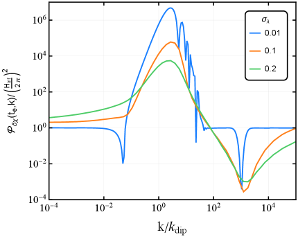
For a fixed $A$, an enlarged $\sigma_{\lambda}$ refers to a dip with a more gentle slope, the enhancement effect from $\lambda_{,\phi}$ becomes weaker. The maximum of the total friction is less than that of a smaller $\sigma_{\lambda}$ (see the evolution of the total friction as shown in the right panel of Fig. 1), which therefore leads to a less enhancement of peak displayed in the right panel of Fig. 4. For a wide dip with $\sigma_{\lambda}=0.2$, the peak amplitude of $\mathcal{P}_{\delta\chi}(t_{\text{e}},k)$ is comparable with the approximation (2.15) shown in the left panel of Fig. 2. However, the shapes of $\mathcal{P}_{\delta\chi}(t_{\text{e}},k)$ are still distinct, due to the effect arising from $\lambda_{,\phi}$. We notice that the first dip prior to the growth becomes shallower ($\sigma_{\lambda}=0.1$) or even disappears for a wider dip ($\sigma_{\lambda}=0.2$). This trend results from the fact that the condition (2.19) occurs at an earlier time for a larger $\sigma_{\lambda}$ (see the right panel of Fig. 1), which results in the growth of “decaying mode” in $\delta\chi$. It dominates over the constant mode at an earlier time (corresponding to a smaller $k$). This fact can also be observed from the slopes of $\mathcal{P}_{\delta\chi}(t_{\text{e}},k)$ in the small-$k$ region for $\sigma_{\lambda}=0.1$ and $\sigma_{\lambda}=0.2$, such that the growth of $\mathcal{P}_{\delta\chi}(t_{\text{e}},k)$ becomes earlier. Additionally, both cases display a broader second dip, which is caused by the fact that the positively large total friction term with a larger $\sigma_{\lambda}$ lasts for a longer time, as shown in the right panel of Fig. 1.

The $\delta\mathcal{N}$ formalism is a powerful tool that enables us to analytically calculate the nonlinear evolutions of scalar perturbations on large scales by solely solving the background equations without any knowledge of complicated perturbation dynamics. This formalism establishes a connection between the superhorzion curvature perturbation on the uniform-density hypersurface and the perturbation in e-folding number between the initial spatially-flat hypersurface $\Sigma_{s}(t_{i})$ and the final uniform-density hypersurface $\Sigma_{u}(t_{f})$, namely

$$\zeta(t_{f},\mathbf{x})=N(t_{i},t_{f};\mathbf{x})-\bar{N}(t_{i},t_{f})~{},$$

(2.21)

where $\bar{N}$ measures the homogeneous expansion from $\Sigma_{s}(t_{i})$ to $\Sigma_{s}(t_{f})$, while $N$ refers to the local expansion from $\Sigma_{s}(t_{i})$ to $\Sigma_{u}(t_{f})$. The non-linear definition of $\zeta$ without imposing $\delta\rho=0$ is given by [53], $\zeta\equiv-\psi+\frac{1}{3}\int_{\bar{\rho}(t)}^{\rho(t,\mathbf{x})}\frac{\mathrm{d}\tilde{\rho}}{\tilde{\rho}+P(\tilde{\rho})}$ along with the parametrization of the full spatial metric $g_{ij}(t,\mathbf{x})=a^{2}(t)e^{2\psi(t,\mathbf{x})}\gamma_{ij}$, where $\psi$ is the non-linear generalization of the linear metric perturbation $\Phi$ shown in Eq. (2.6). In the $\delta\mathcal{N}$ formalism (2.21), the final time $t_{f}$ should be chosen as a moment such that our Universe has already reached the adiabatic limit, i.e., $\zeta$ is time-independent afterward. Hence, we choose $t_{f}$ as the curvaton’s decay since $\zeta$ is conserved after $t_{\text{dec}}$ with a single matter component (radiation) existing in the Universe. For the initial time $t_{i}$, we choose it to be the end of inflation $t_{\text{e}}$ instead of the horizon-crossing usually adopted in other literature (e.g., [55, 39, 56, 29, 33, 57]), since all the scales of interest are well outside the horizon at $t_{\text{e}}$ and the curvaton field $\chi$ has the non-trivial evolution between the horizon-crossing to the end of inflation for non-quadratic potentials [39]. The underlying reason that one can choose the initial time to start the $\delta\mathcal{N}$ calculation “at will” is due to the intriguing property of the $\delta\mathcal{N}$ formalism (2.21), such that it is independent of the initial hypersurface. More importantly, the $\delta\mathcal{N}$ formalism states that one can write the Taylor expansion of the final superhorizon curvature perturbation on $\Sigma_{s}(t_{i})$ as

$$\zeta(\mathbf{x})=N_{,\phi^{a}}\delta\phi^{a}+{1\over 2}N_{,\phi^{a}\phi^{b}}\left[\delta\phi^{a}\delta\phi^{b}-\langle\delta\phi^{a}\delta\phi^{b}\rangle\right]+\mathcal{O}(\delta\phi^{3})~{},$$

(2.22)

where the summation is implied with repeated indices of $\phi^{a}$. For notational simplicity, we drop the time arguments on both sides, and one should keep in mind that all the derivatives and field perturbations are evaluated on the initial hypersurface $\Sigma_{s}(t_{i})$. On the other hand, the local non-Gaussianity of curvature perturbations is described in the following form,

$$\zeta(\mathbf{x})=\zeta_{g}(\mathbf{x})+{3\over 5}f_{\text{NL}}\left[\zeta_{g}^{2}(\mathbf{x})-\langle\zeta_{g}^{2}(\mathbf{x})\rangle\right]+\mathcal{O}(\zeta_{g}^{3})~{},$$

(2.23)

where $\zeta_{g}(\mathbf{x})$ is the Gaussian part of $\zeta(\mathbf{x})$ satisfying the ensemble average $\langle\zeta_{g}\rangle=0$. Hence, matching Eq. (2.23) with Eq. (2.22), one immediately obtains the following relations,

	$\displaystyle\mathcal{P}_{\zeta}$	$\displaystyle=\left(N_{,\phi}\right)^{2}\mathcal{P}_{\delta\phi}+\left(N_{,\chi}\right)^{2}\mathcal{P}_{\delta\chi}~{},$		(2.24)
	$\displaystyle f_{\text{NL}}$	$\displaystyle={5\over 6}{\left(N_{,\phi}\right)^{2}N_{,\phi\phi}+\left(N_{,\chi}\right)^{2}N_{,\chi\chi}\over\left[\left(N_{,\phi}\right)^{2}+\left(N_{,\chi}\right)^{2}\right]^{2}}~{}.$		(2.25)

In the above steps, $\delta\phi$ and $\delta\chi$ are assumed to be uncorrelated random fields at the time of interest. In the following calculations, we also assume that the curvaton field perturbation $\delta\chi_{\text{e}}\equiv\delta\chi(t_{\text{e}})$ is Gaussian, which is reasonable since $\chi$ is assumed to be a light field during inflation, and its field perturbation $\delta\chi$ should be scale-invariant and Gaussian during inflation [58].

In what follows, we shall apply the formalism developed in Ref. [39] to our mixed scenario, which is suitable for a general curvaton’s potential. The most crucial conclusion presented in Ref. [39] is that the statistical properties of curvature perturbations receive the potentially significant correction from the non-uniform onset of curvaton’s oscillation, that typically arises in non-quadratic potentials. The onset of the curvaton’s oscillation is naturally defined as a moment when the time scale of the curvaton rolling becomes comparable to the Hubble time [39], namely $H_{\text{osc}}\equiv\left|\dot{\chi}/\chi\right|$, instead of the usual uniform one $H_{\text{osc}}=m_{\chi}$ for a quadratic potential. In the period $(t_{\text{e}},t_{\text{osc}})$, the radiation is still dominant, and the Hubble friction term is much stronger than the curvaton’s mass term, so that one can use the slow-roll approximation to the curvaton’s evolution in this period [39],

$$5H\dot{\chi}\simeq-V_{,\chi}~{},$$

(2.26)

which is subject to the condition $|V_{,\chi\chi}/5H^{2}|\ll 1$ that holds during the period $(t_{\text{e}},t_{\text{osc}})$ and $\dot{H}/H^{2}=-2$ during the radiation-dominated era. With above preparations, the Hubble parameter at $t_{\text{osc}}$ is identified as a unique function of $\chi_{\text{osc}}$,

$$H_{\text{osc}}^{2}\simeq{V_{,\chi}(\chi_{\text{osc}})\over 5\chi_{\text{osc}}}={1\over 5\chi_{\text{osc}}}f_{a}m_{\chi}^{2}\sin\left({\chi_{\text{osc}}\over f_{a}}\right)~{},$$

(2.27)

which is consistent with $H_{\text{osc}}^{2}\simeq m_{\chi}^{2}$ in the small-field limit $\chi_{\text{osc}}\ll f_{a}$ for the axion-like potential (2.2). Integrating Eq. (2.26), one can obtain the non-linear evolution of the curvaton field in the period $(t_{\text{e}},t_{\text{osc}})$,

$${\partial\chi_{\text{osc}}\over\partial\chi_{\text{e}}}={1\over 1-Y(\chi_{\text{osc}})}{V_{,\chi}(\chi_{\text{osc}})\over V_{,\chi}(\chi_{\text{e}})}~{},$$

(2.28)

where $Y(\chi_{\text{osc}})\equiv{1\over 4}\left({\chi_{\text{osc}}V_{,\chi\chi}(\chi_{\text{osc}})\over V_{,\chi}(\chi_{\text{osc}})}-1\right)={\chi_{\text{osc}}\cot(\chi_{\text{osc}}/f_{a})-f_{a}\over 4f_{a}}$, and we solve Eq. (2.28) as

$$\ln\left|{\tan(\theta_{\text{osc}}/2)\over\tan(\theta_{\text{e}}/2)}\right|=-{\theta_{\text{osc}}\over 4\sin\theta_{\text{osc}}}~{},$$

(2.29)

which is shown by the solid blue curve in the left panel of Fig. 5, and its asymptotic behavior can be written as

$$\theta_{\text{osc}}\simeq\theta_{\text{e}}-0.286\theta_{\text{e}}^{2}+0.086\theta_{\text{e}}^{4}-0.012\theta_{\text{e}}^{6}+0.0006\theta_{\text{e}}^{8}~{},$$

(2.30)

where $\theta\equiv\chi/f_{a}$. Note that this asymptotic expansion is consistent with the fact that the non-linear evolution disappears in the small-field limit $\theta_{\text{e}}\rightarrow 0$, namely $\theta_{\text{osc}}\rightarrow\theta_{\text{e}}$, in contrast to the approximation used in Ref. [39]. The asymptotic expansion (2.30) performs better compared to our numerical results of the power spectrum and non-Gaussianity (see the solid blue curve shown in Fig. 6).

In order to calculate the statistical properties of the final curvature perturbation using the $\delta\mathcal{N}$ formalism (2.24), we need to know the total homogeneous e-folding number from $t_{\text{e}}$ to $t_{\text{dec}}$, namely $N\equiv\ln{a_{\text{dec}}\over a_{\text{e}}}$, and it is divided into two parts,

$$N=N_{\text{osc}}+N_{\text{dec}}~{},$$

(2.31)

where $N_{\text{osc}}=\ln{a_{\text{osc}}\over a_{\text{e}}}={1\over 4}\ln{\rho_{r}^{\text{e}}\over\rho_{r}^{\text{osc}}}$ and $N_{\text{dec}}=\ln{a_{\text{dec}}\over a_{\text{osc}}}={1\over 4}\ln{\rho_{r}^{\text{osc}}\over\rho_{r}^{\text{dec}}}$. Using the Friedmann equation $3M_{\text{Pl}}^{2}H_{\text{osc}}^{2}=\rho_{r}^{\text{osc}}$ at the onset of the curvaton oscillation and $\rho_{\chi}^{\text{dec}}=\rho_{\chi}^{\text{osc}}e^{-3N_{\text{dec}}}$, along with Eqs. (2.27) and (2.28), one can calculate the first and second derivatives of the total e-folding number $N$ as

	$\displaystyle N_{,\chi_{\text{e}}}$	$\displaystyle={\alpha\over 3f_{a}\theta_{\text{osc}}}{\sin\theta_{\text{osc}}\left(4\theta_{\text{osc}}+\theta_{\text{osc}}\cos\theta_{\text{osc}}+3\sin\theta_{\text{osc}}\right)\over\sin\theta_{\text{e}}\left(5\sin\theta_{\text{osc}}-\theta_{\text{osc}}\cos\theta_{\text{osc}}\right)}~{},$		(2.32)
	$\displaystyle N_{,\chi_{\text{e}}\chi_{\text{e}}}$	$\displaystyle={\alpha\over 9f_{a}^{2}}{\left(4\theta_{\text{osc}}+\theta_{\text{osc}}\cos\theta_{\text{osc}}+3\sin\theta_{\text{osc}}\right)^{2}\sin^{2}\theta_{\text{osc}}\over\theta_{\text{osc}}^{2}\sin^{2}\theta_{\text{e}}(-5\sin\theta_{\text{osc}}+\theta_{\text{osc}}\cos\theta_{\text{osc}})^{2}}$
		$\displaystyle\times\Bigg{\{}(1-\alpha)(\alpha+3)+{1\over 3+4\theta_{\text{osc}}\cot{\theta_{\text{osc}}\over 2}-3\theta_{\text{osc}}}\Bigg{[}-3\theta_{\text{osc}}\csc\theta_{\text{osc}}\cos\theta_{\text{e}}\left(5-\theta_{\text{osc}}\cot\theta_{\text{osc}}\right)$
		$\displaystyle+12\theta_{\text{osc}}\cot\theta_{\text{osc}}+12\theta_{\text{osc}}\frac{\cot\theta_{\text{osc}}-\theta_{\text{osc}}\csc^{2}\theta_{\text{osc}}}{5-\theta_{\text{osc}}\cot\theta_{\text{osc}}}$
		$\displaystyle+\frac{3\left(-2\theta_{\text{osc}}^{2}-8\theta_{\text{osc}}^{2}\cos\theta_{\text{osc}}+3\cos(2\theta_{\text{osc}})-3\right)\csc\frac{\theta_{\text{osc}}}{2}\sec\frac{\theta_{\text{osc}}}{2}}{4\theta_{\text{osc}}+3\sin\theta_{\text{osc}}+\theta_{\text{osc}}\cos\theta_{\text{osc}}}\Bigg{]}\Bigg{\}}~{},$		(2.33)

where we defined

$$\alpha\equiv{3\rho_{\chi}\over 3\rho_{\chi}+4\rho_{r}}\Big{|}_{\text{dec}}$$

(2.34)

to characterize the relative density fraction of curvaton at its decay, and manifestly $0\leq\alpha\leq 1$. It is straightforward to check that if we set the uniform-oscillation condition, namely $\rho_{\chi}^{\text{osc}}=m_{\chi}^{2}\chi_{\text{osc}}^{2}$ and $H_{\text{osc}}=m_{\chi}$, the above expressions (2.32) and (2.2.1) reduce to the results found in Ref. [55]: $N_{,\chi_{\text{e}}}=2\alpha g_{,\chi_{\text{e}}}/(3g)$ and $N_{,\chi_{\text{e}}\chi_{\text{e}}}=2\alpha/9\left[\left(3-4\alpha-2\alpha^{2}\right)\left(g_{,\chi_{\text{e}}}/g\right)^{2}+3g_{,\chi_{\text{e}}\chi_{\text{e}}}/g\right]$. Note that the $g$ function here can characterize the non-linear evolution of $\chi$ from $t_{\text{e}}$ to $t_{\text{osc}}$, which is the case for a non-quadratic potential as we have seen in the left panel of Fig. 5.

Finally, we derive the final curvature power spectrum $\mathcal{P}_{\zeta}(t_{\text{dec}},k)$ and the non-linear parameter $f_{\text{NL}}$ at $t_{\text{dec}}$ using Eqs. (2.24) and (2.25), respectively,

	$\displaystyle\mathcal{P}_{\zeta}(t_{\text{dec}},k)$	$\displaystyle=\mathcal{P}_{\delta\phi}(t_{\text{e}},k)+(N_{,\chi_{\text{e}}})^{2}\mathcal{P}_{\delta\chi}(t_{\text{e}},k)$
		$\displaystyle=\mathcal{P}_{\delta\phi}(t_{\text{e}},k)+\left[{2\alpha\over 3f_{a}\theta_{\text{osc}}}F(\theta_{\text{e}},\theta_{\text{osc}})\right]^{2}\mathcal{P}_{\delta\chi}(t_{\text{e}},k)~{},$		(2.35)
	$\displaystyle f_{\text{NL}}$	$\displaystyle={5\over 6}{N_{,\chi\chi}\over\left(N_{,\chi}\right)^{2}}~{},$		(2.36)

where

$$F(\theta_{\text{e}},\theta_{\text{osc}})\equiv{\sin\theta_{\text{osc}}\left(4\theta_{\text{osc}}+\theta_{\text{osc}}\cos\theta_{\text{osc}}+3\sin\theta_{\text{osc}}\right)\over 2\sin\theta_{\text{e}}\left(5\sin\theta_{\text{osc}}-\theta_{\text{osc}}\cos\theta_{\text{osc}}\right)}$$

(2.37)

is defined to describe the deviation from the quadratic potential in terms of the non-linear evolution of $\chi$ during the period $(t_{\text{e}},t_{\text{osc}})$ for the axion-like potential (2.2). This deviation becomes larger when $\chi_{e}$ approaches the hilltop of the axion-like potential [39], as shown by the solid blue curve in the right panel of Fig. 5. Since the curvaton oscillation epoch will be significantly delayed, causing more contribution to $N_{,\chi_{\text{e}}}$ and $N_{,\chi_{\text{e}}\chi_{\text{e}}}$. From the left and right panels of Fig. 6, our analytic results (solid blue curves) are comparable to the numerical results (the numerical method will be presented later) and perform better than the analytic formulas used in Ref. [57]. Meanwhile, to satisfy the constraint on $f_{\text{NL}}$, namely $f_{\text{NL}}=-0.9\pm 5.1$ (Planck $68\%$ confidence level) [59], $\chi_{e}$ must be away from $\pi f_{a}$. It follows from the right panel of Fig. 6 that the curvaton field value at the end of inflation lies in the range $0<\theta_{\text{e}}\lesssim 3$ for $\alpha\rightarrow 1$. It is also known that $f_{\text{NL}}$ would be significantly enhanced if the curvaton is still subdominant when it decays [39]. Hence, the current constraint on $f_{\text{NL}}$ favors $\alpha\rightarrow 1$, namely the curvaton already dominates when it decays. In addition, the perturbativity condition also suggests the smallness of $f_{\text{NL}}$ [60, 61]. For the above considerations and simplicity, we do not consider the non-Gaussianity in our model, and the curvaton field value is thus determined from the right panel of Fig. 6 such that $\theta_{\text{e}}\simeq 2$. Consequently, there is a slight difference in the peak amplitude of $\mathcal{P}_{\zeta}(t_{\text{dec}},k)$ for the axion-like and quadratic curvaton potentials, see the right panel of Fig. 5 and the left panel of Fig. 6.

It follows from the left panel of Fig. 6 and the expression (2.2.1), the peak of the final curvature spectrum $\mathcal{P}_{\zeta}(t_{\text{dec}},k)$ is thus approximately enhanced by a factor $10^{-1}(M_{\text{Pl}}/f_{a})^{2}$ compared to the peak of $\mathcal{P}_{\delta\chi}(t_{\text{e}},k)$ shown in Fig. 2. The left panel of Fig. 2 also implies that $\mathcal{P}_{\zeta}(t_{\text{dec}},k)$ on large scales will be dominated by $\delta\chi$ if $10^{-1}(M_{\text{Pl}}/f_{a})^{2}>10^{3}$, namely $f_{a}<10^{-2}M_{\text{Pl}}$, which is favored by the concrete particle models [57, 33]. Hence, we focus on this parameter region in this paper, namely the final curvature power spectrum on all scales are dominated by the contribution from the curvaton, and consequently, two dips of $\mathcal{P}_{\delta\chi}(t_{\text{e}},k)$ shown in Fig. 2 and Fig. 4 also display to some extent in the final curvature spectra $\mathcal{P}_{\zeta}(t_{\text{dec}},k)$ as shown in Fig. 7.

Employing the sudden-decay approximation, the full background equations are written as

	$\displaystyle 3M_{\mathrm{Pl}}^{2}H^{2}=\rho_{r}+\rho_{\chi}~{},$		(2.38)
	$\displaystyle\rho_{\chi}={1\over 2}\dot{\chi}^{2}+V_{\text{cur}}(\chi)~{},$		(2.39)
	$\displaystyle\dot{\rho}_{r}+4H\rho_{r}=0~{},$		(2.40)
	$\displaystyle\ddot{\chi}+3H\dot{\chi}+V_{\text{cur},\chi}=0~{}.$		(2.41)

Taking the change of variables, namely $N=\ln a(t)$ and $x\equiv m_{\chi}t$, we obtain two independent equations [62],

	$\displaystyle N^{\prime}=\left\{Ae^{-4N}+B\left[{1\over 2}(\theta^{\prime})^{2}+\tilde{V}(\theta)\right]\right\}^{1/2}~{},$		(2.42)
	$\displaystyle\theta^{\prime\prime}+3N^{\prime}\theta^{\prime}+{\mathrm{d}\tilde{V}(\theta)\over\mathrm{d}\theta}=0~{},$		(2.43)

where the prime denotes the derivative with respect to $x$, and $\tilde{V}(\theta)\equiv V_{\text{cur}}(\chi)/(f_{a}^{2}m_{\chi}^{2})=1-\cos\theta$, $A\equiv{\rho_{r,e}\over 3M_{\mathrm{Pl}}^{2}m_{\chi}^{2}}$ and $B\equiv{f_{a}^{2}\over 3M_{\mathrm{Pl}}^{2}}$. Here $\rho_{r,e}$ is the radiation energy density at the end of inflation. The numerical results of $N_{,\theta_{\text{e}}}$ and $f_{\text{NL}}$ are shown by black thick solid curves in Fig. 6. Then, we derive the final curvature spectrum $\mathcal{P}_{\zeta}(t_{\text{dec}},k)$ as shown in Fig. 7, in terms of four sets of parameters: $\left\{\phi_{\text{dip}}/M_{\text{Pl}}=4.8,\sigma_{\lambda}=0.01\right\}$ (the blue curve); $\left\{\phi_{\text{dip}}/M_{\text{Pl}}=4.5,\sigma_{\lambda}=0.01\right\}$ (the black curve); $\left\{\phi_{\text{dip}}/M_{\text{Pl}}=5.0,\sigma_{\lambda}=0.01\right\}$ (the purple curve); $\left\{\phi_{\text{dip}}/M_{\text{Pl}}=4.8,\sigma_{\lambda}=0.1\right\}$ (the green curve), and the rest parameters are the same with Fig. 2.

References

- Akrami et al. [2020a] Y. Akrami et al. (Planck), Astron. Astrophys. 641, A10 (2020a), arXiv:1807.06211 [astro-ph.CO] .
- Hawking [1971] S. Hawking, Mon. Not. Roy. Astron. Soc. 152, 75 (1971).
- Carr and Hawking [1974] B. J. Carr and S. W. Hawking, Mon. Not. Roy. Astron. Soc. 168, 399 (1974).
- Carr [1975] B. J. Carr, Astrophys. J. 201, 1 (1975).
- Carr et al. [2010] B. J. Carr, K. Kohri, Y. Sendouda, and J. Yokoyama, Phys. Rev. D 81, 104019 (2010), arXiv:0912.5297 [astro-ph.CO] .
- Carr et al. [2021] B. Carr, K. Kohri, Y. Sendouda, and J. Yokoyama, Rept. Prog. Phys. 84, 116902 (2021), arXiv:2002.12778 [astro-ph.CO] .
- Luo et al. [2021] Y. Luo, C. Chen, M. Kusakabe, and T. Kajino, JCAP 05, 042 (2021), arXiv:2011.10937 [astro-ph.CO] .
- Cai et al. [2022] Y.-F. Cai, C. Chen, Q. Ding, and Y. Wang, Eur. Phys. J. C 82, 464 (2022), arXiv:2105.11481 [astro-ph.CO] .
- Cai et al. [2021] Y.-F. Cai, C. Chen, Q. Ding, and Y. Wang, (2021), arXiv:2112.10422 [astro-ph.CO] .
- Bean and Magueijo [2002] R. Bean and J. Magueijo, Phys. Rev. D 66, 063505 (2002), arXiv:astro-ph/0204486 .
- Kawasaki et al. [2012] M. Kawasaki, A. Kusenko, and T. T. Yanagida, Phys. Lett. B 711, 1 (2012), arXiv:1202.3848 [astro-ph.CO] .
- Yuan et al. [2023] G.-W. Yuan, L. Lei, Y.-Z. Wang, B. Wang, Y.-Y. Wang, C. Chen, Z.-Q. Shen, Y.-F. Cai, and Y.-Z. Fan, (2023), arXiv:2303.09391 [astro-ph.CO] .
- Cai et al. [2023] Y.-F. Cai, C. Tang, G. Mo, S. Yan, C. Chen, X. Ma, B. Wang, W. Luo, D. Easson, and A. Marciano, (2023), arXiv:2301.09403 [astro-ph.CO] .
- Bird et al. [2016] S. Bird, I. Cholis, J. B. Muñoz, Y. Ali-Haïmoud, M. Kamionkowski, E. D. Kovetz, A. Raccanelli, and A. G. Riess, Phys. Rev. Lett. 116, 201301 (2016), arXiv:1603.00464 [astro-ph.CO] .
- Sasaki et al. [2016] M. Sasaki, T. Suyama, T. Tanaka, and S. Yokoyama, Phys. Rev. Lett. 117, 061101 (2016), [Erratum: Phys.Rev.Lett. 121, 059901 (2018)], arXiv:1603.08338 [astro-ph.CO] .
- Jedamzik [2020] K. Jedamzik, JCAP 09, 022 (2020), arXiv:2006.11172 [astro-ph.CO] .
- Carr and Kuhnel [2020] B. Carr and F. Kuhnel, Ann. Rev. Nucl. Part. Sci. 70, 355 (2020), arXiv:2006.02838 [astro-ph.CO] .
- Green and Kavanagh [2021] A. M. Green and B. J. Kavanagh, J. Phys. G 48, 043001 (2021), arXiv:2007.10722 [astro-ph.CO] .
- Escrivà et al. [2022] A. Escrivà, F. Kuhnel, and Y. Tada, (2022), arXiv:2211.05767 [astro-ph.CO] .
- Pi and Sasaki [2021] S. Pi and M. Sasaki, (2021), arXiv:2112.12680 [astro-ph.CO] .
- Meng et al. [2022a] D.-S. Meng, C. Yuan, and Q.-G. Huang, (2022a), arXiv:2212.03577 [astro-ph.CO] .
- Kawasaki et al. [1998] M. Kawasaki, N. Sugiyama, and T. Yanagida, Phys. Rev. D 57, 6050 (1998), arXiv:hep-ph/9710259 .
- Choudhury and Mazumdar [2014] S. Choudhury and A. Mazumdar, Phys. Lett. B 733, 270 (2014), arXiv:1307.5119 [astro-ph.CO] .
- Byrnes et al. [2019] C. T. Byrnes, P. S. Cole, and S. P. Patil, JCAP 06, 028 (2019), arXiv:1811.11158 [astro-ph.CO] .
- Carrilho et al. [2019] P. Carrilho, K. A. Malik, and D. J. Mulryne, Phys. Rev. D 100, 103529 (2019), arXiv:1907.05237 [astro-ph.CO] .
- Cole et al. [2022] P. S. Cole, A. D. Gow, C. T. Byrnes, and S. P. Patil, (2022), arXiv:2204.07573 [astro-ph.CO] .
- Dimopoulos et al. [2003] K. Dimopoulos, D. H. Lyth, A. Notari, and A. Riotto, JHEP 07, 053 (2003), arXiv:hep-ph/0304050 .
- Kasuya and Kawasaki [2009] S. Kasuya and M. Kawasaki, Phys. Rev. D 80, 023516 (2009), arXiv:0904.3800 [astro-ph.CO] .
- Kawasaki et al. [2013] M. Kawasaki, N. Kitajima, and T. T. Yanagida, Phys. Rev. D 87, 063519 (2013), arXiv:1207.2550 [hep-ph] .
- Ando et al. [2018a] K. Ando, K. Inomata, M. Kawasaki, K. Mukaida, and T. T. Yanagida, Phys. Rev. D 97, 123512 (2018a), arXiv:1711.08956 [astro-ph.CO] .
- Ando et al. [2018b] K. Ando, M. Kawasaki, and H. Nakatsuka, Phys. Rev. D 98, 083508 (2018b), arXiv:1805.07757 [astro-ph.CO] .
- Inomata et al. [2021] K. Inomata, M. Kawasaki, K. Mukaida, and T. T. Yanagida, Phys. Rev. Lett. 126, 131301 (2021), arXiv:2011.01270 [astro-ph.CO] .
- Kawasaki and Nakatsuka [2021] M. Kawasaki and H. Nakatsuka, JCAP 05, 023 (2021), arXiv:2101.11244 [astro-ph.CO] .
- Linde and Mukhanov [1997] A. D. Linde and V. F. Mukhanov, Phys. Rev. D 56, R535 (1997), arXiv:astro-ph/9610219 .
- Lyth and Wands [2002] D. H. Lyth and D. Wands, Phys. Lett. B 524, 5 (2002), arXiv:hep-ph/0110002 .
- Lyth et al. [2003] D. H. Lyth, C. Ungarelli, and D. Wands, Phys. Rev. D 67, 023503 (2003), arXiv:astro-ph/0208055 .
- Malik et al. [2003] K. A. Malik, D. Wands, and C. Ungarelli, Phys. Rev. D 67, 063516 (2003), arXiv:astro-ph/0211602 .
- Malik and Lyth [2006] K. A. Malik and D. H. Lyth, JCAP 09, 008 (2006), arXiv:astro-ph/0604387 .
- Kawasaki et al. [2011] M. Kawasaki, T. Kobayashi, and F. Takahashi, Phys. Rev. D 84, 123506 (2011), arXiv:1107.6011 [astro-ph.CO] .
- Gomez-Reino and Scrucca [2006] M. Gomez-Reino and C. A. Scrucca, JHEP 09, 008 (2006), arXiv:hep-th/0606273 .
- Covi et al. [2008a] L. Covi, M. Gomez-Reino, C. Gross, J. Louis, G. A. Palma, and C. A. Scrucca, JHEP 06, 057 (2008a), arXiv:0804.1073 [hep-th] .
- Covi et al. [2008b] L. Covi, M. Gomez-Reino, C. Gross, J. Louis, G. A. Palma, and C. A. Scrucca, JHEP 08, 055 (2008b), arXiv:0805.3290 [hep-th] .
- Lalak et al. [2007] Z. Lalak, D. Langlois, S. Pokorski, and K. Turzynski, JCAP 07, 014 (2007), arXiv:0704.0212 [hep-th] .
- Armendariz-Picon et al. [1999] C. Armendariz-Picon, T. Damour, and V. F. Mukhanov, Phys. Lett. B 458, 209 (1999), arXiv:hep-th/9904075 .
- Armendariz-Picon et al. [2001] C. Armendariz-Picon, V. F. Mukhanov, and P. J. Steinhardt, Phys. Rev. D 63, 103510 (2001), arXiv:astro-ph/0006373 .
- Domènech and Sasaki [2015] G. Domènech and M. Sasaki, JCAP 04, 022 (2015), arXiv:1501.07699 [gr-qc] .
- De Angelis and van de Bruck [2023] M. De Angelis and C. van de Bruck, (2023), arXiv:2304.12364 [hep-th] .
- Lola et al. [2021] S. Lola, A. Lymperis, and E. N. Saridakis, Eur. Phys. J. C 81, 719 (2021), arXiv:2005.14069 [gr-qc] .
- Choudhury et al. [2023a] S. Choudhury, S. Panda, and M. Sami, (2023a), arXiv:2302.05655 [astro-ph.CO] .
- Choudhury et al. [2023b] S. Choudhury, S. Panda, and M. Sami, (2023b), arXiv:2304.04065 [astro-ph.CO] .
- Starobinsky [1985] A. A. Starobinsky, JETP Lett. 42, 152 (1985).
- Sasaki and Stewart [1996] M. Sasaki and E. D. Stewart, Prog. Theor. Phys. 95, 71 (1996), arXiv:astro-ph/9507001 .
- Lyth et al. [2005] D. H. Lyth, K. A. Malik, and M. Sasaki, JCAP 05, 004 (2005), arXiv:astro-ph/0411220 .
- Abolhasani et al. [2019] A. A. Abolhasani, H. Firouzjahi, A. Naruko, and M. Sasaki, Delta N Formalism in Cosmological Perturbation Theory (WSP, 2019).
- Sasaki et al. [2006] M. Sasaki, J. Valiviita, and D. Wands, Phys. Rev. D 74, 103003 (2006), arXiv:astro-ph/0607627 .
- Ichikawa et al. [2008] K. Ichikawa, T. Suyama, T. Takahashi, and M. Yamaguchi, Phys. Rev. D 78, 023513 (2008), arXiv:0802.4138 [astro-ph] .
- Kobayashi [2020] T. Kobayashi, Phys. Rev. Lett. 125, 011302 (2020), arXiv:2005.01741 [astro-ph.CO] .
- Maldacena [2003] J. M. Maldacena, JHEP 05, 013 (2003), arXiv:astro-ph/0210603 .
- Akrami et al. [2020b] Y. Akrami et al. (Planck), Astron. Astrophys. 641, A9 (2020b), arXiv:1905.05697 [astro-ph.CO] .
- Kristiano and Yokoyama [2022] J. Kristiano and J. Yokoyama, Phys. Rev. Lett. 128, 061301 (2022), arXiv:2104.01953 [hep-th] .
- Meng et al. [2022b] D.-S. Meng, C. Yuan, and Q.-g. Huang, Phys. Rev. D 106, 063508 (2022b), arXiv:2207.07668 [astro-ph.CO] .
- Huang [2010] Q.-G. Huang, JCAP 11, 026 (2010), [Erratum: JCAP 02, E01 (2011)], arXiv:1008.2641 [astro-ph.CO] .
- Bird et al. [2011] S. Bird, H. V. Peiris, M. Viel, and L. Verde, Mon. Not. Roy. Astron. Soc. 413, 1717 (2011), arXiv:1010.1519 [astro-ph.CO] .
- Fixsen et al. [1996] D. J. Fixsen, E. S. Cheng, J. M. Gales, J. C. Mather, R. A. Shafer, and E. L. Wright, Astrophys. J. 473, 576 (1996), arXiv:astro-ph/9605054 .
- Musco et al. [2021] I. Musco, V. De Luca, G. Franciolini, and A. Riotto, Phys. Rev. D 103, 063538 (2021), arXiv:2011.03014 [astro-ph.CO] .
- Salopek and Bond [1990] D. S. Salopek and J. R. Bond, Phys. Rev. D 42, 3936 (1990).
- Deruelle and Langlois [1995] N. Deruelle and D. Langlois, Phys. Rev. D 52, 2007 (1995), arXiv:gr-qc/9411040 .
- Afshordi and Brandenberger [2001] N. Afshordi and R. H. Brandenberger, Phys. Rev. D 63, 123505 (2001), arXiv:gr-qc/0011075 .
- Shibata and Sasaki [1999] M. Shibata and M. Sasaki, Phys. Rev. D 60, 084002 (1999), arXiv:gr-qc/9905064 .
- Kawasaki and Nakatsuka [2019] M. Kawasaki and H. Nakatsuka, Phys. Rev. D 99, 123501 (2019), arXiv:1903.02994 [astro-ph.CO] .
- Young et al. [2019] S. Young, I. Musco, and C. T. Byrnes, JCAP 11, 012 (2019), arXiv:1904.00984 [astro-ph.CO] .
- Kalaja et al. [2019] A. Kalaja, N. Bellomo, N. Bartolo, D. Bertacca, S. Matarrese, I. Musco, A. Raccanelli, and L. Verde, JCAP 10, 031 (2019), arXiv:1908.03596 [astro-ph.CO] .
- Yoo et al. [2018] C.-M. Yoo, T. Harada, J. Garriga, and K. Kohri, PTEP 2018, 123E01 (2018), arXiv:1805.03946 [astro-ph.CO] .
- De Luca et al. [2019] V. De Luca, G. Franciolini, A. Kehagias, M. Peloso, A. Riotto, and C. Ünal, JCAP 07, 048 (2019), arXiv:1904.00970 [astro-ph.CO] .
- Gow et al. [2021] A. D. Gow, C. T. Byrnes, P. S. Cole, and S. Young, JCAP 02, 002 (2021), arXiv:2008.03289 [astro-ph.CO] .
- Germani and Musco [2019] C. Germani and I. Musco, Phys. Rev. Lett. 122, 141302 (2019), arXiv:1805.04087 [astro-ph.CO] .
- Musco [2019] I. Musco, Phys. Rev. D 100, 123524 (2019), arXiv:1809.02127 [gr-qc] .
- Sasaki et al. [2018] M. Sasaki, T. Suyama, T. Tanaka, and S. Yokoyama, Class. Quant. Grav. 35, 063001 (2018), arXiv:1801.05235 [astro-ph.CO] .
- Press and Schechter [1974] W. H. Press and P. Schechter, Astrophys. J. 187, 425 (1974).
- Ananda et al. [2007] K. N. Ananda, C. Clarkson, and D. Wands, Phys. Rev. D 75, 123518 (2007), arXiv:gr-qc/0612013 .
- Baumann et al. [2007] D. Baumann, P. J. Steinhardt, K. Takahashi, and K. Ichiki, Phys. Rev. D 76, 084019 (2007), arXiv:hep-th/0703290 .
- Domènech [2021] G. Domènech, Universe 7, 398 (2021), arXiv:2109.01398 [gr-qc] .
- Janssen et al. [2015] G. Janssen et al., PoS AASKA14, 037 (2015), arXiv:1501.00127 [astro-ph.IM] .
- Ruan et al. [2020] W.-H. Ruan, Z.-K. Guo, R.-G. Cai, and Y.-Z. Zhang, Int. J. Mod. Phys. A 35, 2050075 (2020), arXiv:1807.09495 [gr-qc] .
- Kawamura et al. [2011] S. Kawamura et al., Class. Quant. Grav. 28, 094011 (2011).
- Crowder and Cornish [2005] J. Crowder and N. J. Cornish, Phys. Rev. D 72, 083005 (2005), arXiv:gr-qc/0506015 .
- Baker et al. [2019] J. Baker et al., (2019), arXiv:1907.06482 [astro-ph.IM] .
- El-Neaj et al. [2020] Y. A. El-Neaj et al. (AEDGE), EPJ Quant. Technol. 7, 6 (2020), arXiv:1908.00802 [gr-qc] .
- Garcia-Bellido et al. [2021] J. Garcia-Bellido, H. Murayama, and G. White, JCAP 12, 023 (2021), arXiv:2104.04778 [hep-ph] .
- Sesana et al. [2021] A. Sesana et al., Exper. Astron. 51, 1333 (2021), arXiv:1908.11391 [astro-ph.IM] .
- Kohri and Terada [2018] K. Kohri and T. Terada, Phys. Rev. D 97, 123532 (2018), arXiv:1804.08577 [gr-qc] .
- Espinosa et al. [2018] J. R. Espinosa, D. Racco, and A. Riotto, JCAP 09, 012 (2018), arXiv:1804.07732 [hep-ph] .
- Brill and Hartle [1964] D. R. Brill and J. B. Hartle, Phys. Rev. 135, B271 (1964).
- Isaacson [1968a] R. A. Isaacson, Phys. Rev. 166, 1263 (1968a).
- Isaacson [1968b] R. A. Isaacson, Phys. Rev. 166, 1272 (1968b).
- Ford and Parker [1977] L. H. Ford and L. Parker, Phys. Rev. D 16, 1601 (1977).
- Ota et al. [2022] A. Ota, H. J. Macpherson, and W. R. Coulton, Phys. Rev. D 106, 063521 (2022), arXiv:2111.09163 [gr-qc] .
- Pi and Sasaki [2020] S. Pi and M. Sasaki, JCAP 09, 037 (2020), arXiv:2005.12306 [gr-qc] .