Group-Theoretic Wideband Radar Waveform Design

The analytical theory of radar signal processing employs cross-correlation technique for target detection and parameter estimation [1, 2]. The radar’s ability to distinguish closely-spaced targets is completely specified by the ambiguity function (AF) of its transmit waveform. Through the AF, the transmit waveform enters into the performance analyses related to detection, target parameter accuracy, and resolution of multiple closely-spaced targets. The AF was first introduced by Ville [3] and its significance as a signal design metric in the mathematical radar theory is credited to Woodward [4, 5], later expounded in detail by Siebert [6]. The AF is not uniquely defined, including in the works of Woodward, which focused on narrowband waveforms [2, 7, 8, 9].

However, many radar applications such as for ground penetration [10], synthetic apertures [11], and vehicular sensing systems [12] employ wideband waveforms that yield higher range resolution and improved interference suppression. Unlike the narrowband AF (NAF), the Doppler effect on the envelopes of transmit signal reflected off the targets is not constant across the bandwidth. This led to several generalizations of Woodward’s definition to wideband ambiguity function (WAF) [13, 14, 15]. In this paper, we focus on such wideband interpretations of AF.

There is a large body of research on using the AF as an aid to select suitable radar waveforms. An AF equal to zero except at one point is ideal for detection tasks [16, Chapter 3]. But, in this case, the probability of the target lying within the response region would be near zero [17]. In the absence of an ideal AF, significant theoretical efforts have been devoted to the problem of finding functions of delay and Doppler that are not only realizable as AFs but also have suitable radar performance. The resulting procedure of waveform design has traditionally focused on achieving AFs that are thumbtack with a sharp central spike and low sidelobes in the delay-Doppler plane. The inverse problem - given an AF, design a signal that yields it - is traced back to the 1970 work by Rudolf de Buda. This study claimed that when the NAF is bounded by a Hermite function, then the signal is also a Hermite function where the polynomial is found from its AF by comparing coefficients [18]. Later works such as [19] extended de Buda’s results by showing that the bounding assumption over the radar AF is removed to uniquely identify (up to trivial ambiguities) a Hermite function and rectangular pulse trains. More recently, phase retrieval techniques have been applied to estimate a band-limited signal from its NAF [8].

The interest in studying both NAF and WAF in a unified framework resulted in analyzing these functions from the perspective of a group representation theory [20]. The NAF and WAF are coefficients of the unitary representations of their respective groups. For example, for the NAF, the delayed and Doppler-shifted replicas of a signal are obtained by a unitary operator that is a member of a Heisenberg group [21]. On the other hand, the time dilated and delayed replicas result from the transmit signal through a unitary operator that comes from an affine group. The wideband cross-AFs are, therefore, affine wavelet transforms [20].

In this paper, we investigate group-theoretic formulations to design signals that obey a given WAF. Similar prior works were largely limited to analyzing the NAF. In [21], using the theory developed in [22] for the extraspecial 2-group, it was shown that finite Heisenberg-Weyl groups provide a unifying framework for several sequences to design narrowband phase-coded radar waveforms. Later, this was expanded to design complementary sequences in [23, 24]. Initial investigations into the group representation theory for WAF appeared in [25, 20, 26]. This was expanded to include Mellin transform in [27]. Nearly all of the aforementioned works did not examine the design of wideband waveforms from a given WAF using group-theoretic tools. In this work, we build upon the unitary representation of WAF to design complementary sequences. In particular, we exploit the seminal work of [28, 29] to build a tight frame, whose bounding constants are then utilized to obtain low WAF sidelobes. We show that the resulting tight frame is related to the wavelet transform that defines the WAF.

The rest of the paper is organized as follows. In the next section, we introduce the definitions of WAF. We then make a connection with affine groups in Section III. We analytically design the signal using this theory in Section IV before concluding in Section V. Throughout the paper, for reference, the NAF of an uncoded pulse $w(t)$ with duration $T_{c}$ and unit energy $\int_{-\frac{T_{c}}{2}}^{\frac{T_{c}}{2}}|w(t)|^{2}dt=1$ is the inner product of the transmit waveform $w(t)$ and its time-delayed/frequency-shifted version:

$\displaystyle\psi_{w}(\tau,\nu)=\int_{-\frac{T_{c}}{2}}^{\frac{T_{c}}{2}}w(t)w^{*}(t-\tau)e^{-j\nu t}dt,$

(1)

where $(\tau,\nu)$ are the delay-Doppler coordinates.

As a traveling wavefield reflects off a moving target, the field either expands or compresses in time because of the movement of the target. When a narrowband waveform is transmitted, this compressive effect is ignored for the waveform’s complex envelope and only considered for the carrier. The WAF for which this approximation is not permissible is

$\displaystyle\chi_{w}^{1}(\tau,\nu)=\sqrt{\gamma}\int_{-\frac{T_{c}}{2}}^{\frac{T_{c}}{2}}w(t)w^{*}(\gamma(t-\tau))e^{-j\nu t}dt,$

(2)

where the factor $\gamma=1+f_{v}/f_{c}$ accounts for the stretching/compressing in time of the reflected signal (Doppler factor). Assume $f_{0}$ to be the central frequency of the spectra $W(\nu)$. Denote

	$\displaystyle\Delta f$	$\displaystyle=\nu-f_{0},$	$\displaystyle\textit{ frequency deviation},$
	$\displaystyle\delta$	$\displaystyle=\frac{2v}{c+v},$	$\displaystyle\textit{the relative velocity}.$

Then,

	$\displaystyle w(\gamma(t-\tau))$	$\displaystyle=e^{-2\pi jf_{0}\delta(t-\tau)}$
		$\displaystyle\times\int_{-\frac{T_{c}}{2}}^{\frac{T_{c}}{2}}W(\nu)e^{2\pi j\nu(t-\tau)}e^{-2\pi j\Delta f\delta(t-\tau)}d\nu.$		(3)

Observe that there are two factors affecting the signal behaviour in time $e^{-2\pi jf_{0}\delta(t-\tau)}$ and $e^{-2\pi j\Delta f\delta(t-\tau)}$. The first shifts the signal spectra; the second accounts for the stretching/compressing in time of the reflected signal. If the target-source velocity $v\ll c$ then $\delta\ll 1$ and thus $e^{-2\pi j\Delta f\delta(t-\tau)}\approx 1$. In this case,

$\displaystyle w(\gamma(t-\tau))=e^{-2\pi jf_{0}(\gamma-1)(t-\tau)}w(t-\tau).$

(4)

It follows from (4) that the WAF is, equivalently,

$\displaystyle\chi_{w}^{1}(\tau,\nu)=\sqrt{\gamma}e^{-2\pi jf_{0}(\gamma-1)\tau}\int_{-\frac{T_{c}}{2}}^{\frac{T_{c}}{2}}w(t)w^{*}(t-\tau)e^{-j\nu t}dt.$

(5)

There is a scalar term in front of the integral to account for a change in amplitude of the reflected signal as it is stretched. The amplitude scaling is necessary for the conservation of energy when the waveform is stretched in time.

Note that, like its narrowband counterpart, the definition of WAF is also not unique. The form in (5) (hereafter, $\chi_{w}(\tau,\nu)$) is due to Kelly-Wishner [14] and Altes [30, 31]. A second form appears as wavelets in the works by Daubechies [28]; Auslander and Gertner [25]; Miller [32]:

$\displaystyle\chi_{w}^{2}(\tau,\nu)=\frac{1}{\sqrt{\gamma}}\int_{-\frac{T_{c}}{2}}^{\frac{T_{c}}{2}}w(t)w^{\ast}\left(\frac{t-\tau}{\gamma}\right)e^{-j\nu t}dt.$

(6)

Speiser [13] and Chaiyasena et al. [26] deal with the following WAF, where the dilation is inside the integral:

$\displaystyle\chi_{w}^{3}(\tau,\nu)=\sqrt{\gamma}\int_{-\frac{T_{c}}{2}}^{\frac{T_{c}}{2}}w(t)w^{\ast}(\gamma t-\tau)e^{-j\nu t}dt.$

(7)

In [33, 34], the dilation is included as an exponential (similar to a Doppler shift):

$\displaystyle\chi_{w}^{4}(\tau,\nu)=e^{\frac{\nu}{2}}\int_{-\frac{T_{c}}{2}}^{\frac{T_{c}}{2}}w(t)w^{\ast}\left(e^{-\nu}t-\tau\right)e^{-j\nu t}dt.$

(8)

In this paper, we concern ourselves with the definition in (5).

Consider a baseband waveform constructed by phase coding translates of $w(t)$ with a unimodular sequence $x[n]$ of length $L$ as

$$x(t)=\sum_{\ell=0}^{L-1}x[\ell]w\left(t-\ell T_{c}\right),$$

with the energy

$\displaystyle E_{x}$

$\displaystyle=\int_{\mathbb{R}}|x(t)|^{2}dt=\left(\sum_{\ell=0}^{L-1}x[\ell]^{2}\right)\int_{-\frac{T_{c}}{2}}^{\frac{T_{c}}{2}}|w(t)|^{2}dt=L.$

The WAF $\chi_{x}(\tau,\nu)$ of $x(t)$ becomes

	$\displaystyle\chi_{x}(\tau,\nu)$	$\displaystyle=\sqrt{\gamma}\int_{-\frac{T_{c}}{2}}^{\frac{T_{c}}{2}}x(t)x^{\ast}(\gamma(t-\tau))e^{-j\nu t}dt$
		$\displaystyle=\sqrt{\gamma}\int_{-\frac{T_{c}}{2}}^{\frac{T_{c}}{2}}\sum_{\ell,\ell^{\prime}=0}^{L-1}x[\ell]w\left(t-\ell T_{c}\right)x^{*}[\ell^{\prime}]$
		$\displaystyle\hskip 80.00012pt\times w^{*}\left(\gamma t-\gamma\tau-\ell^{\prime}T_{c}\right)e^{-j\nu t}dt$
		$\displaystyle=\sum_{\ell,k=0}^{L-1}A_{x}^{\ell}\left(k,\nu T_{c}\right)\chi_{w}\left(\tau-\frac{T_{c}(k+\ell(\gamma-1))}{\gamma},\nu\right),$		(9)

where $\displaystyle A_{x}^{\ell}\left(k,\nu T_{c}\right)=x[\ell]x^{*}[\ell-k]e^{-j\nu\ell T_{c}}$.

Next, we extend WAF to complementary sequence pair [24]. Denote a binary sequence of length $N$ by $P=\left\{p_{n}\right\}_{n=0}^{N-1}$ and the complement of $p_{n}$ by $\bar{p}_{n}=1-p_{n}$. The $P$-pulse train $x_{P}(t)$ transmitted at a pulse repetition interval $T$ is

$\displaystyle x_{P}(t)=\sum_{n=0}^{N-1}p_{n}x(t-nT)+\bar{p}_{n}\tilde{x}(t-nT).$

(10)

Multiplying (10) by a discrete-valued real nonnegative sequence $Q=\left\{q_{n}\right\}_{n=0}^{N-1}$, $\left(q_{n}\geq 0\right)$ of length $N$ gives the $Q$-pulse train $x_{Q}(t)$ is

$\displaystyle x_{Q}(t)=\sum_{n=0}^{N-1}q_{n}\left[p_{n}x(t-nT)+\bar{p}_{n}\tilde{x}(t-nT)\right].$

(11)

Transmitting $x_{P}(t)$ and correlating the return with $x_{Q}(t)$ yields

	$\displaystyle\chi_{PQ}(\tau,\nu)$	$\displaystyle=\int_{\mathbb{R}}x_{P}(t)x_{Q}^{\ast}(\gamma(t-\tau))e^{-j\nu t}dt$		(12)
		$\displaystyle\approx\frac{1}{\sqrt{\gamma}}\sum_{n=0}^{N-1}q_{n}e^{-j\nu nT}\left[p_{n}\chi_{x}(\tau,\nu)+\bar{p}_{n}\chi_{\tilde{x}}(\tau,\nu)\right],$		(13)

where range aliases at offset $\pm nT,n=$ $1,2,\ldots,N-1$ are ignored and the last approximation follows from the fact that $\nu\ll 1/T$ so that the phase rotation within one coherent processing interval (CPI) (slow time) can be approximated as a constant. Our goal is to obtain the sequences $p_{n}$ and $q_{n}$ from a given WAF.

The WAF in (2) is related to a representation of the affine or $a\cdot x+b$ group. The $a\cdot x+b$ group is a set $\mathbb{R}\setminus\{0\}\times\mathbb{R}$ equipped with the product

$\displaystyle(a,b)\circ(a^{\prime},b^{\prime})=(a\cdot a^{\prime},b+a\cdot b^{\prime}).$

(14)

The unity of the group is $(1,0)$ because

	$\displaystyle(1,0)\circ(a,b)$	$\displaystyle=(a,b)$
	$\displaystyle(a,b)\circ(1,0)$	$\displaystyle=(a,b).$		(15)

The right and left inverse of $(a,b)$ is $\left(\frac{1}{a},-\frac{b}{a}\right)$ since

	$\displaystyle(a,b)\circ\left(\frac{1}{a},-\frac{b}{a}\right)$	$\displaystyle=(1,0)$
	$\displaystyle\left(\frac{1}{a},-\frac{b}{a}\right)\circ(a,b)$	$\displaystyle=(1,0).$		(16)

The group is non-commutative

	$\displaystyle(a,b)\circ(a^{\prime},b^{\prime})$	$\displaystyle=(a\cdot a^{\prime},b+a\cdot b^{\prime})$
	$\displaystyle(a^{\prime},b^{\prime})\circ(a,b)$	$\displaystyle=(a\cdot a^{\prime},b^{\prime}+a^{\prime}\cdot b).$		(17)

From the definition of this group, we now introduce unitary representation.

Difference sets have been well studied in the combinatorial design theory [36, 37]. They are known to exist for certain cases and a comprehensive repository of difference sets is provided in [38]. As an illustration of our approach, we employ the Singer difference sets [39] to design the sequences $p_{n}$ and $q_{n}$ in (11).

Consider the prime number $q=11$ and a power constant $d=2$. Then, the size of the sequences is directly determined from these values as

$$N=\frac{q^{d+1}-1}{q-1}=133.$$

Define $C_{1}=\frac{q^{d}-1}{q-1}$ and $C_{2}=\frac{q^{d-1}-1}{q-1}$. This yields a $(N,C_{1},C_{2})$-difference set. Under this setup, the resultant difference set is

$\displaystyle\mathcal{F}=\{0,1,8,14,30,45,47,56,66,106,109,129\}.$

(41)

From (33), the WAF in (13) corresponds to the inner product between $x_{P}$ and $x_{Q}$. The function uses the product $p_{n}q_{n}$ as

	$\displaystyle\left\lvert\langle x_{P},x_{Q}^{(1/\gamma,\tau)}\rangle\right\rvert\equiv\chi_{PQ}(\tau,\nu)$
	$\displaystyle\approx\frac{1}{\sqrt{\gamma}}\sum_{n=0}^{N-1}q_{n}e^{-j\nu nT}\left[p_{n}\chi_{x}(\tau,\nu)+\bar{p}_{n}\chi_{\tilde{x}}(\tau,\nu)\right]$
	$\displaystyle\leq\frac{1}{\sqrt{\gamma}}\sum_{n=0}^{N-1}q_{n}p_{n}\lvert\chi_{x}(\tau,\nu)\rvert+q_{n}(1-p_{n})\lvert\chi_{\tilde{x}}(\tau,\nu)\rvert.$		(42)

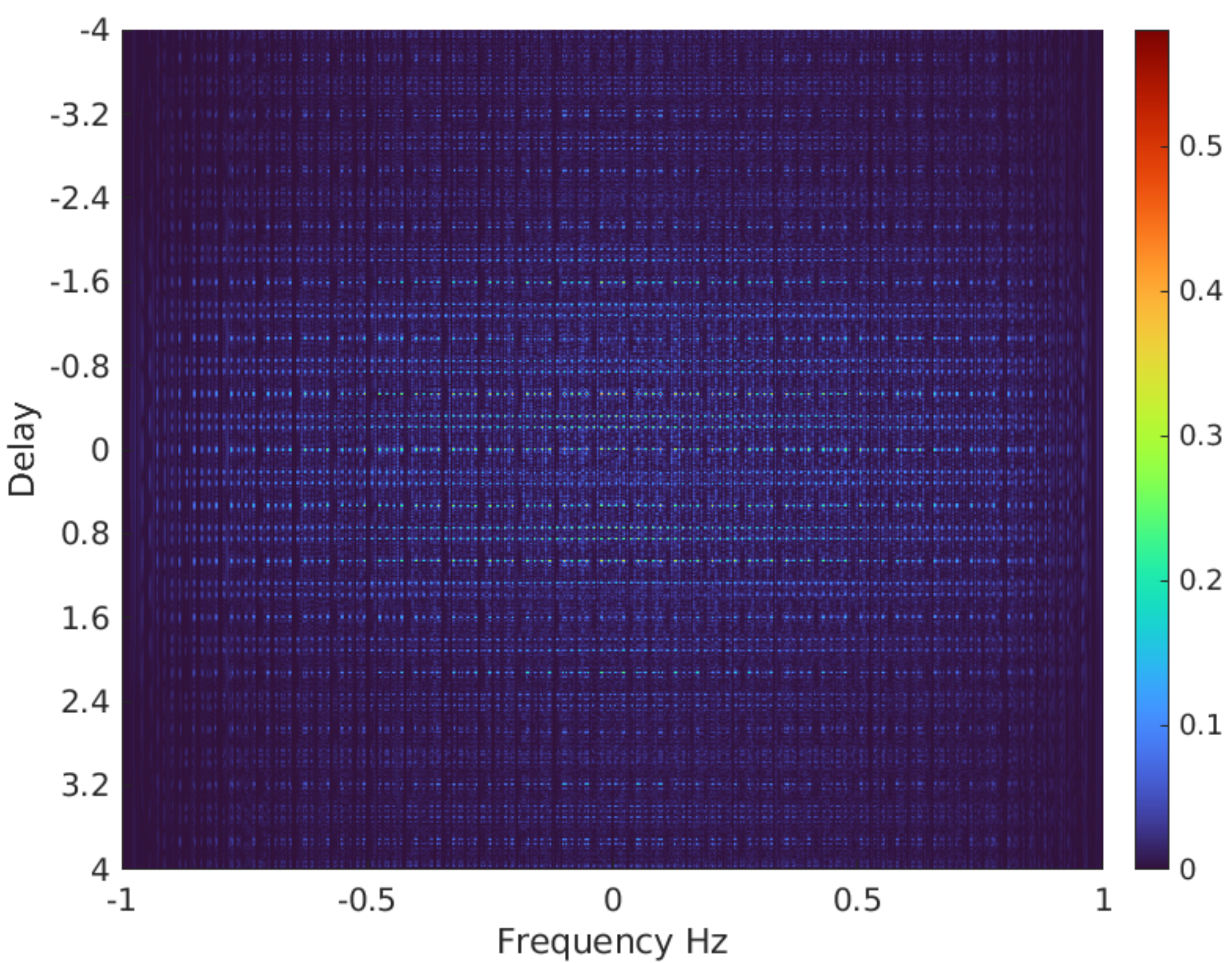
Therefore, in order to minimize the ratio $B/A$ of the resultant frame applied to $x_{Q}$ (following the strategy explained in the previous section), we need to design $p_{n}q_{n}$. To this end, we set $p_{n}q_{n}=1$ for all $n\in\mathcal{F}$, and $p_{n}q_{n}=0$ for all $n\in\{0,\dots,N\}\setminus\mathcal{F}$. From these constraints, we can determine $(p_{n},q_{n})$ as

$$(p_{n},q_{n})=\left\{\begin{array}[]{ll}(1,1)&\text{ if }n\in\mathcal{F}\\ (n\mod 2,n+1\mod 2)&\text{ if }n\not\in\mathcal{F}\end{array}\right..$$

(45)

The resultant wideband cross-AF is plotted in Fig. 1.

In the context of tight frames in [40, 41], it has been shown that, if the Welch bound is reached, with overwhelming probability we are able to guarantee the reconstruction. It turns out that difference sets can provide patterns that reach the Welch bound [35]. For the particular scenario we considered, this bound is $\mu=\sqrt{\frac{N-C_{1}}{C_{1}(N-1)}}=\sqrt{\frac{121}{1584}}\approx 0.27$. Therefore, $\frac{B}{A}=1+\mathcal{O}(\mu)$. We remark that this strategy is limited by the calculation of the difference set in (41), which is computationally demanding. In the future, we intend to develop a numerical algorithm to estimate new difference sets to produce higher values of $N$.

We analytically demonstrated design procedure a wideband radar waveform using group-theoretic strategy via difference sets. We first mathematically expressed the waveform’s WAF as a coefficient function of the unitary representation of the group $a\cdot x+b$. From this representation, we connected the wavelet expansions of frame to the WAF. This allowed us to derive a strategy to design two binary sequences in order to minimize the ratio of the bounding constant of the wavelet frame so constructed. The analytical estimation of these bounds is usually computationally expensive. As an alternative, we targeted achieving the Welch bound using difference sets. Our proposed group-theoretic waveform design guarantees a near-optimal reconstruction.

References

- [1] N. Levanon and E. Mozeson, Radar signals. John Wiley & Sons, 2004.
- [2] P. Z. Peebles, Radar Principles. Wiley-Interscience, 1998.
- [3] J. Ville, “Théorie et application dela notion de signal analytique,” Câbles et transmissions, vol. 2, no. 1, pp. 61–74, 1948, in French.
- [4] P. M. Woodward, Probability and information theory, with applications to radar, 3rd ed., ser. International Series of Monographs on Electronics and Instrumentation. McGraw-Hill, 1965.
- [5] ——, “Radar ambiguity analysis,” Royal Radar Establishment, Malvern, UK, Tech. Rep. RRE-TN-731, 1967.
- [6] W. Siebert, “A radar detection philosophy,” IRE Transactions on Information Theory, vol. 2, no. 3, pp. 204–221, 1956.
- [7] J. George, K. V. Mishra, C. M. Nguyen, and V. Chandrasekar, “Implementation of blind zone and range-velocity ambiguity mitigation for solid-state weather radar,” in IEEE Radar Conference, 2010, pp. 1434–1438.
- [8] S. Pinilla, K. V. Mishra, B. M. Sadler, and H. Arguello, “BanRAW: Band-limited radar waveform design via phase retrieval,” in IEEE International Conference on Acoustics, Speech and Signal Processing, 2021, pp. 5449–5453.
- [9] S. Pinilla, K. V. Mishra, and B. Sadler, “WaveMax: FrFT-based convex phase retrieval for radar waveform design,” in IEEE International Symposium on Information Theory, 2021, pp. 2387–2392.
- [10] F. Giovanneschi, K. V. Mishra, M. A. Gonzalez-Huici, Y. C. Eldar, and J. H. Ender, “Dictionary learning for adaptive GPR landmine classification,” IEEE Transactions on Geoscience and Remote Sensing, vol. 57, no. 12, pp. 10 036–10 055, 2019.
- [11] P. Vouras, K. V. Mishra, A. Artusio-Glimpse, S. Pinilla, A. Xenaki, D. W. Griffith, and K. Egiazarian, “An overview of advances in signal processing techniques for classical and quantum wideband synthetic apertures,” arXiv preprint arXiv:2205.05602, 2022.
- [12] K. V. Mishra, M. B. Shankar, V. Koivunen, B. Ottersten, and S. A. Vorobyov, “Toward millimeter-wave joint radar communications: A signal processing perspective,” IEEE Signal Processing Magazine, vol. 36, no. 5, pp. 100–114, 2019.
- [13] J. Speiser, “Wide-band ambiguity functions (Corresp.),” IEEE Transactions on Information Theory, vol. 13, no. 1, pp. 122–123, 1967.
- [14] E. Kelly and R. Wishner, “Matched-filter theory for high-velocity, accelerating targets,” IEEE Transactions on Military Electronics, vol. 9, no. 1, pp. 56–69, 1965.
- [15] A. W. Rihaczek, “Delay-Doppler ambiguity function for wideband signals,” IEEE Transactions on Aerospace and Electronic Systems, no. 4, pp. 705–711, 1967.
- [16] M. Jankiraman, Design of multi-frequency CW radars. SciTech Publishing, 2007, vol. 2.
- [17] A. W. Rihaczek, Principles of high-resolution radar. Artech House, 1996.
- [18] R. de Buda, “Signals that can be calculated from their ambiguity function,” IEEE Transactions on Information Theory, vol. 16, no. 2, pp. 195–202, 1970.
- [19] P. Jaming, “The phase retrieval problem for the radar ambiguity function and vice versa,” in IEEE Radar Conference, 2010, pp. 230–235.
- [20] A. P. Chaiyasena, L. H. Sibul, A. Banyaga, and M. L. Fowler, “Wavelet transforms and signal ambiguity functions,” in Asilomar Conference on Signals, Systems and Computers, vol. 2, 1990, p. 1084.
- [21] S. D. Howard, A. R. Calderbank, and W. Moran, “The finite Heisenberg-Weyl groups in radar and communications,” EURASIP Journal on Advances in Signal Processing, vol. 2006, pp. 1–12, 2006.
- [22] A. R. Calderbank, P. J. Cameron, W. M. Kantor, and J. J. Seidel, “-Kerdock codes, orthogonal spreads, and extremal Euclidean line-sets,” Proceedings of the London Mathematical Society, vol. 75, no. 2, pp. 436–480, 1997.
- [23] A. Pezeshki, A. R. Calderbank, W. Moran, and S. D. Howard, “Doppler resilient Golay complementary waveforms,” IEEE Transactions on Information Theory, vol. 54, no. 9, pp. 4254–4266, 2008.
- [24] W. Dang, A. Pezeshki, S. D. Howard, W. Moran, and R. Calderbank, “Coordinating complementary waveforms for suppressing range sidelobes in a Doppler band,” arXiv preprint arXiv:2001.09397, 2020.
- [25] L. Auslander and I. Gertner, “Wide-band ambiguity function and group,” in Signal Processing Part I: Signal Processing Theory, ser. IMA Volumes in Mathematics and its Applications, L. Auslander, F. A. Grúnbaum, W. Helton, T. Kailath, P. Khargonekar, and S. Mitter, Eds. Springer-Verlag, 1990, vol. 22, p. 1–12.
- [26] A. Chaiyasena, L. Sibul, and A. Banyaga, “Wavelet transforms, wideband ambiguity functions and group theory,” in Asilomar Conference on Signals, Systems & Computers, 1992, pp. 140–141.
- [27] R. G. Shenoy and T. W. Parks, “Wide-band ambiguity functions and affine wigner distributions,” Signal Processing, vol. 41, no. 3, pp. 339–363, 1995.
- [28] I. Daubechies, “Time-frequency localization operators: A geometric phase space approach,” IEEE Transactions on Information Theory, vol. 34, no. 4, pp. 605–612, 1988.
- [29] ——, “The wavelet transform, time-frequency localization and signal analysis,” IEEE transactions on information theory, vol. 36, no. 5, pp. 961–1005, 1990.
- [30] R. A. Altes, “Methods of wideband signal design for radar and sonar systems,” Ph.D. dissertation, The University of Rochester, 1970.
- [31] ——, “Some invariance properties of the wide-band ambiguity function,” The Journal of the Acoustical Society of America, vol. 53, no. 4, pp. 1154–1160, 1973.
- [32] W. Miller Jr., “Topics in harmonic analysis with applications to radar and sonar, Part 1,” in Radar and Sonar Part I, ser. IMA Volumes in Mathematics and its Applications, R. E. Blahut, W. Miller Jr., and C. H. Wilcox, Eds. Springer-Verlag, 1991, vol. 32, p. 99.
- [33] C. E. Heil and D. F. Walnut, “Continuous and discrete wavelet transforms,” SIAM Review, vol. 31, no. 4, pp. 628–666, 1989.
- [34] M. L. Fowler, “Signal detection using time-frequency and time-scale methods,” Ph.D. dissertation, The Pennsylvania State University, 1991.
- [35] P. Xia, S. Zhou, and G. B. Giannakis, “Achieving the welch bound with difference sets,” IEEE Transactions on Information Theory, vol. 51, no. 5, pp. 1900–1907, 2005.
- [36] J. H. Dinitz and D. R. Stinson, Contemporary design theory: A collection of Surveys. John Wiley & Sons, 1992, vol. 26.
- [37] M. Aigner, Combinatorial theory. Springer Science & Business Media, 2012.
- [38] La Jolla Difference Set Repository, 2021. [Online]. Available: https://www.dmgordon.org/diffset/
- [39] J. Singer, “A theorem in finite projective geometry and some applications to number theory,” Transactions of the American Mathematical Society, vol. 43, no. 3, pp. 377–385, 1938.
- [40] J. A. Tropp, “On the conditioning of random subdictionaries,” Applied and Computational Harmonic Analysis, vol. 25, no. 1, pp. 1–24, 2008.
- [41] C. Mosher, S. Kaplan, and F. Janiszewski, “Non-uniform optimal sampling for seismic survey design,” in EAGE Conference and Exhibition, 2012, pp. cp–293.