Group Sparse Optimization for Inpainting of Random Fields on the Sphere 111This work was partly supported by Hong Kong Research Grant Council PolyU15300120 and the Shenzhen Research Institute of Big Data Grant 2019ORF01002.
Abstract
We propose a group sparse optimization model
for inpainting of a square-integrable isotropic random field on the unit sphere,
where the field is represented by spherical harmonics with random complex coefficients. In the proposed optimization model, the variable is an infinite-dimensional complex vector and the objective function is a real-valued function defined by a hybrid of the norm and non-Liptchitz norm that preserves rotational invariance property and group structure of the random complex coefficients.
We show that the infinite-dimensional optimization problem is equivalent to a convexly-constrained finite-dimensional optimization problem.
Moreover, we propose a smoothing penalty algorithm to solve the finite-dimensional problem via unconstrained optimization problems.
We provide an approximation error bound of the inpainted random field defined by a scaled KKT point of the constrained optimization problem
in the square-integrable space on the sphere with probability measure.
Finally, we conduct numerical experiments on band-limited random fields on the sphere and images from Earth topography data to show the promising performance of the smoothing penalty algorithm for inpainting of random fields on the sphere.
Keywords:
group sparse optimization; exact penalty; smoothing method; random field.
1 Introduction
Let be a probability space, and let be the Borel sigma algebra on the unit sphere , where is the norm. A real-valued random field on is an -measurable function , and it is said to be -weakly isotropic if the expected value and covariance of are rotationally invariant (see [14]). It is known that a -weakly isotropic random field on the sphere has the following Karhunen-Loève (K-L) expansion [23, 25],
| (1.1) |
where are random spherical harmonic coefficients of , , for , are spherical harmonics with degree and order , and is the surface measure on satisfying For convenient, let
denote the coefficient vector of an isotropic random field . The infinite-dimensional coefficient vector can be grouped according to degrees and written in the following group structure
| (1.2) |
where
From [14], we know that for any given degree and any , the sum
is rotationally invariant, while is not invariant under rotation of the coordinate axes. Moreover, in [14] the angular power spectrum is given by
if the expected value for all . In the study of isotropic random fields [12, 23, 25], the angular power spectrum plays an important role since it contains full information of the covariance of the field and provides characterization of the field. Hence, considering the group structure (1.2) of the coefficients of an isotropic random field is essential.
Sparse representation of a random field is an approximation of with few non-zero elements of . In group sparse representation, instead of considering elements individually, we seek an approximation of with few non-zero groups of , i.e., few non-zero entries of the following vector
In recent years, sparse representation of isotropic random fields has been extensively studied. In [6] the authors studied the sparse representation of random fields via an -regularized minimization problem. In [14], the authors considered isotropic group sparse representation of Gaussian and isotropic random fields on the sphere through an unconstrained optimization problem with a weighted norm, which is an example of group Lasso [34]. In [24], the authors proposed a non-Lipschitz regularization problem with a weighted () norm for the group sparse representation of isotropic random fields. The non-Lipschitz regularizer also preserves the rotational invariance property of for any given degree and any .
Isotropic random fields on the sphere have many applications [5, 20, 26, 28, 31], especially in the study of the Cosmic Microwave Background (CMB) analysis [1, 30]. However, the true spherical random field usually presents masked regions and missing observations. Many inpainting methods [1, 13, 30, 32] have been proposed for recovering the true field based on sparse representation. However, they did not take the group structure (1.2) of the coefficients into consideration.
Group sparse optimization models have been successfully used in signal processing, imaging sciences and predictive analysis [3, 11, 18, 17, 27]. In this paper, we propose a constrained group sparse optimization model for inpainting of isotropic random fields on the sphere based on group structure (1.2). Moreover, to recover the true random field by using information only on a subset which contains an open set, we need the unique continuation property [19] of any realization of a random field, that is, for any fixed , if the value of a field equals to zero on , then the random field is identically zero on the sphere (see Appendix A for more details).
Let be the space on the product space with product measure and the induced norm , where is the space of square-integrable functions over endowed with the inner product
and the induced -norm . By Fubini’s theorem, for , , -a.s., where “-a.s.” stands for almost surely with probability . For brevity, we write as or if no confusion arises.
Let the observed field be given by
| (1.3) |
where is the true isotropic random field that we aim to recover, is observational noise and is an inpainting operator defined by
| (1.4) |
where is a nonempty inpainting area and the set has an open subset. In our optimization model, we consider the observed field as one realization of a random field. For notational simplicity, let
| (1.5) |
denote the spherical harmonic coefficient vector of an isotropic random field for a fixed , where , .
By Parseval’s theorem, we have
Hence the sequence , where is the space of square-summable sequences. We write to indicate .
The number of non-zero groups of with group structure (1.5) is calculated by
where and is called norm of . The norm is discontinuous and does not ensure . In [14], the authors used a weighted norm of defined by
where . It is easy to see that . The norm has been widely used in sparse approximation [11, 18]. In this paper, we use a weighted norm of . Let
be a weighted () space with positive weights and for , where is a constant. For a fixed , we consider the following constrained optimization problem
| (1.6) |
where .
A feasible field of problem (1.6) takes the form
Since , for , there is a finite number such that , where and . Let for , , then . From the definition of , we have
Thus, the feasible set of problem (1.6) is nonempty. Moreover the objective function of problem (1.6) is continuous and level-bounded. Hence an optimal solution of problem (1.6) exists.
Since implies that , we assume , which implies that is not a feasible field of problem (1.6).
Our main contributions are summarized as follows.
-
•
Based on the K-L expansion, the constraint of problem (1.6) can be written in a discrete form with variables . We derive a lower bound for the norm of nonzero groups of scaled KKT points of (1.6). Based on the lower bound, we prove that the infinite-dimensional problem (1.6) is equivalent to a finite-dimensional optimization problem.
-
•
We propose a penalty method for solving the finite-dimensional optimization problem via unconstrained optimization problems. We establish the exact penalization results regarding local minimizers and -minimizers. Moreover, we propose a smoothing penalty algorithm and prove that the sequence generated by the algorithm is bounded and any accumulation point of the sequence is a scaled KKT point of the finite-dimensional optimization problem.
-
•
We give the approximation error of the random field represented by scaled KKT points of the finite-dimensional optimization problem in
The rest of this paper is organised as follows. In Section 2, we prove that the infinite-dimensional discrete optimization problem is equivalent to a finite-dimensional problem. In Section 3, we present the penalty method and give exact penalization results. In Section 4, we discuss optimality conditions of the finite-dimensional optimization problem and its penalty problem. Moreover, we propose a smoothing penalty algorithm and establish its convergence. In Section 5, we give the approximation error in In Section 6, we conduct numerical experiments on band-limited random fields and images from Earth topography data to compare our approach with some existing methods on the quality of the solutions and inpainted images. Finally, we give conclusion remarks in Section 7.
2 Discrete formulation of problem (1.6)
In this section, we propose the discrete formulation of problem (1.6) and prove that the discrete problem is equivalent to a finite-dimensional problem (2.5).
Based on the definition of and the spherical harmonic expansion of , we obtain that
| (2.1) |
where is an infinite-dimensional matrix with with , and
The minimization problem (1.6) can be written as the following optimization problem
| (2.2) |
From the setting of in problem (1.6) and Theorem 8, the feasible set of (2.2) has an interior point and bounded. The following assumption follows from our assumption on problem (1.6).
Assumption 1.
The feasible set of problem (2.2) does not contain .
Note that the objective function and constraint function in (2.2) are real-valued functions with complex variables. Thus, following [24], we apply the Wirtinger calculus (See Appendix B for more details) in this paper.
Since the objective function in problem (2.2) is not Lipschitz continuous at points containing zero groups. We shall consider first-order stationary points of (2.2) and extend the definition of scaled KKT points for finite-dimensional optimization problem with real variables in [8, 10, 29].
Definition 1.
We call a scaled KKT point of (2.2), if there exists such that
| (2.3) |
From (2.3), for any nonzero vector , we have
and . Then,
By definition of and feasibility of , there exists such that . Hence for any nonzero vector , we have
| (2.4) |
By definition of , , we obtain that
which implies that is a finite set. Thus, the number of nonzero vectors of a scaled KKT point of problem (2.2) is finite and there exists an such that . Therefore, the infinite-dimensional problem (2.2) can be truncated to a finite-dimensional problem and approximated in a finite-dimensional space.
For notational simplicity, we truncate to , where . We use to denote the truncated vector whose elements are the first elements of and to denote the leading principal submatrix of order of . Since has an open subset, we have for any nonzero . Thus, the matrix is positive definite.
The truncated finite-dimensional problem of problem (2.2) has the following version
| (2.5) |
By the definition of , the feasible set of (2.5) is nonempty and has an interior point. The objective function is continuous, nonnegative with , and differentiable except at points containing zero groups. The penalty formulation for (2.5) is
| (2.6) |
for some , where . For any nontrivial solution of (2.6), we have
| (2.7) |
3 Exact penalization
In this section, we consider the relationship between problems (2.5) and (2.6). We first give some notations. For a closed set , denotes the distance from a point to and denotes a closed ball with radius and center . Let be defined as
for , and . We denote the feasible set of problem (2.5) by Let .
Since is positive definite, is strongly convex and has a unique global minimizer which implies that Since is strongly convex and quadratic, there is such that for . Choosing such that , from [29, Theorem 9.48], we obtain the following lemma.
Lemma 1.
There exists a constant such that for any ,
Theorem 1.
Proof.
Let be a local minimizer of problem (2.5), that is there exists a neighborhood of such that for . We denote the group support set of by , and the complement set of in by . Let and denote the restrictions of onto and , respectively. We obtain that is a local minimizer of the following problem
| (3.1) |
Let . Then, there exists a small such that is a local minimizer of (3.1) and for all . Let
Let be the vector with and It is easy to see that and By Lemma 1, for all .
The objective function of (3.1) is Lipschitz continuous on . Then by [8, Lemma 3.1], there exists a such that, for any , is a local minimizer of the following problem
that is, there exists a neighborhood of with such that
We now show that is a local minimizer of (2.6) with .
For fixed and , we consider problem (2.6) in the neighborhood , where . Let be a Lipschitz constant of the function over . There exists an such that whenever , ,
| (3.2) |
Hence for any , we have
where the first inequality follows from the Lipschitz continuity of with Lipschitz constant and (3.2), and the last inequality follows from the local optimality of . Thus, is a local minimizer of problem (2.6) with . This completes the proof. ∎
Theorem 2.
Proof.
Note that is a strongly convex function and is a minimizer of . Since the feasible set of (2.5) has an interior point, we have .
By the global optimality of , we have and
| (3.3) |
Hence for any , we obtain
where the first inequality is from the global optimality of , the second inequality is from Lemma 2.4 in [8], the fifth inequality is from the concavity of function for , the sixth inequality is from Lemma 1, the seventh inequality is from (3.3) and the last inequality follows from the choice of . Thus, the projection is an -minimizer of (2.5). This completes the proof. ∎
4 Optimality conditions and a smoothing penalty algorithm
In this section, we first define first-order optimality conditions of (2.5) and (2.6), which are necessary conditions for local optimality. We also derive lower bounds for the norm of nonzero groups of first-order stationary points of (2.5) and (2.6). Next we propose a smoothing penalty algorithm for solving (2.5) and prove its convergence to a first-order stationary point of (2.5).
4.1 First-order optimality conditions
We first present a first-order optimality condition of problem (2.6).
Definition 2.
Theorem 3.
Proof.
The next theorem gives a lower bound for the norm of nonzero groups of stationary points of (2.6).
Theorem 4.
Let be a scaled first-order stationary point of (2.6) and for some . Then,
The proof is similar with that of (2.4), and thus we omit it here. According to Theorems 1 and 3, Theorem 4 gives a lower bound for the norm of nonzero groups of local minimizers of problem (2.5).
Next, we consider the first-order optimality condition of problem (2.5). Similar to Definition 1, we call is a scaled first-order stationary point or a scaled KKT point of (2.5) if the following conditions hold,
| (4.4) |
Since is not a feasible point, thus . Hence, replacing by in Theorem 4, we can obtain a lower bound for the norm of nonzero groups of the scaled KKT point of problem (2.5).
Theorem 5.
Proof.
Let be a local minimizer of problem (2.5), then is a local minimizer of problem (3.1). Recall , then .
The condition that there exists such that implies that if . Thus the LICQ (linear independence constraint qualification) holds at for problem (3.1).
Note that, the objective function of problem (3.1) and are continuously differentiable at and Hence is a KKT point of (3.1), that is, there exists such that
| (4.5) |
Multiplying on both sides of the first equality in (4.5), we obtain
Since for , we obtain
Combining this with (4.5) and , we find that is a scaled KKT point of (2.5). The proof is completed. ∎
From the definitions we can see that for some , any scaled KKT point of problem (2.5) is a scaled first order stationary point of (2.6). Moreover, any scaled first order stationary point of problem (2.6) which belongs to the feasible set is a scaled KKT point of problem (2.5).
4.2 A smoothing penalty algorithm for problem (2.5)
We define a smoothing function of the nonsmooth function as follows
with and is a smoothing parameter. It is easy to verify that and , It is not hard to show that
and
| (4.6) |
By Wirtinger calculus, we obtain where and
More details about the smoothing function can be found in [7] and references therein.
We consider the following optimization problem
| (4.7) |
For fixed positive parameters and , is continuous and level-bounded since is level-bounded and is nonnegative. Moreover, the gradient of is Lipschitz continuous.
Now, we propose a smoothing penalty algorithm for solving problem (2.5).
We give the convergence of Algorithm 4.2 in the following theorem.
Theorem 6.
Proof.
(i) We can see that
where the first inequality follows from that , the second inequality follows from step (1) of Algorithm 4.2, and the equality is from and . Since is level-bounded, is bounded.
(ii) Let be an accumulation point of and be a subsequence of such that as , . Note that
where the first inequality follows from (4.6). Then, we have
| (4.9) |
From step (3) in Algorithm 4.2, and , as , . Taking limits in (4.9) as , , we obtain that . Hence, .
From (4.8), we have
| (4.10) |
We first assume that . For all sufficiently large , we obtain and (4.10) becomes
Taking limits on both sides of the above relation, we obtain which contradicts to Assumption 1. Thus, .
Let for notational simplicity, we have . Then (4.10) reduces to
| (4.11) |
Now, we prove that is bounded. On the contrary, we assume is unbounded and , then,
Passing to the limit in the above relation gives
Since implies is in , but is not a minimizer of , we have and . Moreover, implies that and . Thus, is bounded. Let . Taking limits on both sides of (4.11) gives
Therefore, is a scaled KKT point of (2.5). ∎
5 Approximation error
In [14], the authors gave the approximation error for random field using regularized model based on the observed random field . In this section, we estimate the approximation error of the inpainted random field in the space based on the observed random field .
For any fixed , let with the group support set be a scaled KKT point of problem (2.5). By our results in the previous sections, is a finite number. Moreover, is a scaled KKT point of problem (2.2) in the infinite-dimensional space .
Lemma 2.
If the random variable has finite second order moment that is and there is such that , , then
Proof.
Let be fixed. Since for any ,
we have
Hence, we obtain
where the last inequality follows from . Thus, ∎
Theorem 7.
Let be the observed random field. Then for any there exists such that
where .
Proof.
Since , by Fubini’s theorem, for , , -a.s., in which case admits an expansion in terms of spherical harmonics, -a.s., that is, -a.s., where is the Fourier coefficient vector of .
By Definition 1 for any , , we have . Now, we prove that there exists a positive scalar such that for any . On the contrary, if there exists a such that , then from
we have which is a contradiction with . Thus, from and (2.4), there exists a positive scalar such that for any . Thus, for any there exists such that for any , which implies that
By Lemma 2, for any there exists such that . Let , and .
For notational simplicity, let , where , and , where . Let , we have
| (5.2) |
where the first equality follows from the second equality in (2.3) with for any . For any fixed , by Definition 1 for a scaled KKT point of problem (2.2), there is such that
From (2.1), for , . Thus, for any fixed ,
| (5.3) |
We obtain
| (5.4) |
Thus,
| (5.5) |
where the first equality follows from (5.4) and the first inequality follows from that . Combining (5.2) and (5.5), we obtain
The proof is completed. ∎
6 Numerical experiments
In this section, we conduct numerical experiments to compare the - optimization model (2.5) with the optimization model (31) in [32] on the inpainting of banded-limited random fields and images from Earth topography data to show the efficiency of problem (2.5) and Algorithm 4.2.
Following [8], we adapt the nonmonotone proximal gradient (NPG) method to solve subproblem (4.7) in Algorithm 4.2. For completeness, we present the NPG method as follows.
NPG method for problem (4.7)
For the NPG method to solve (4.7) in Algorithm 4.2 at , we set , , , , , , and for any ,
Algorithm 6 is terminated when
In Algorithm 4.2, we set , , , , . The smoothing penalty algorithm is terminated when where is updated by instead of in the experiments. All codes were written in MATLAB and the realizations were implemented in Python.
6.1 Random data
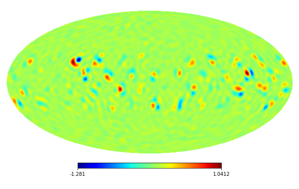
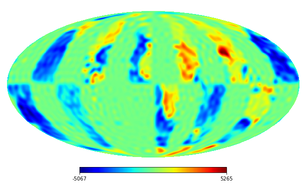
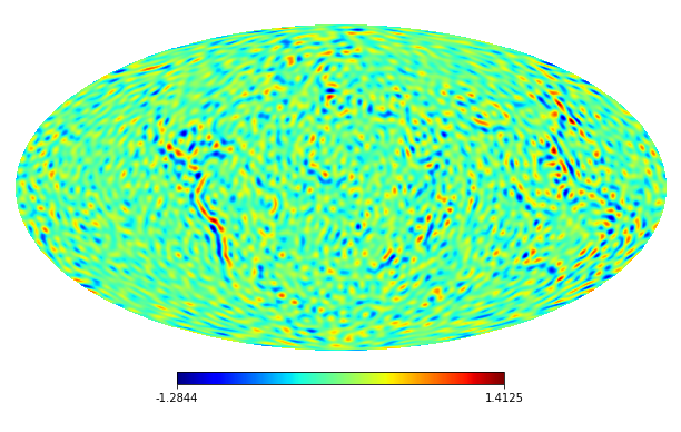
In the following experiments, we consider randomly generated instances which are generated as follows. First, we choose a subset and generate a group sparse coefficient vector such that if and if , where is the coefficient vector with maximum degree of the CMB 2018 map computed by the HEALPy package [15].
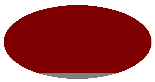
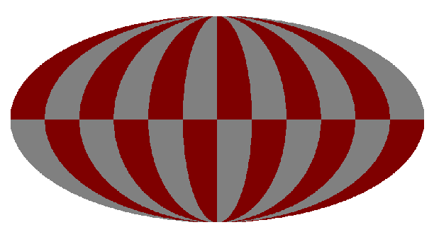
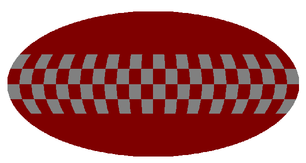
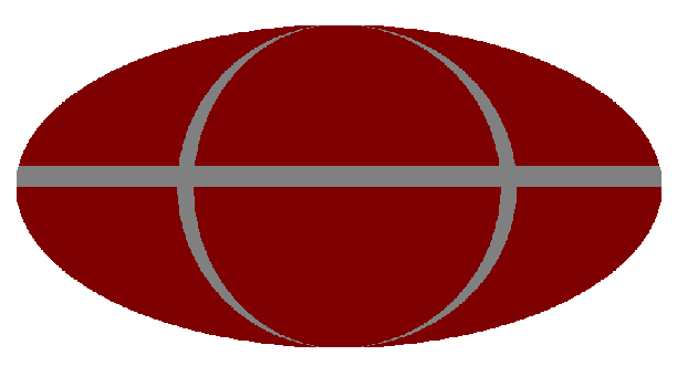
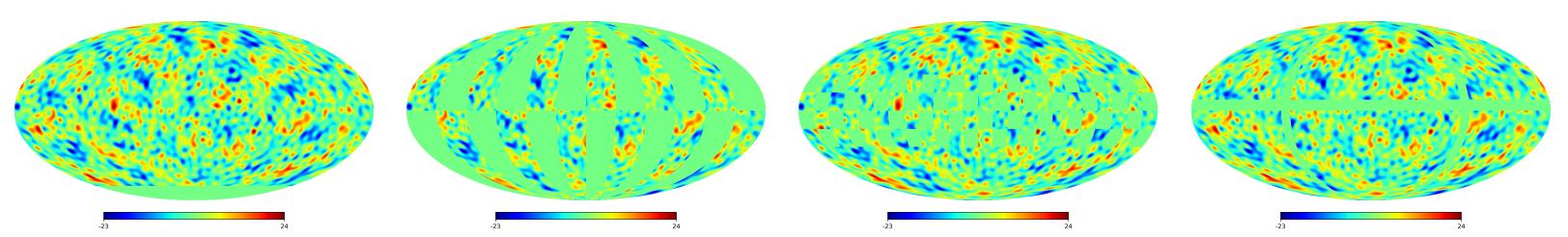
We assume that the noise also has the K-L expansion and set . We generate the data for the noise on the HEALPix points with by the MATLAB command: , where and is a scaling parameter. Then we use the Python HEALPy package to compute the coefficients of the noise. The masks denoted by are shown in Figure 1.
In the experiments, we set , for and . We compare the - optimization model (2.5) by using Algorithm 4.2 with the optimization model (31) in [32] using the YALL1 method [33] under the KKM sampling scheme [21]. We also compare our method with the group SPGl1 method (https://friedlander.io/spgl1/). We present the results in Tables 1 and 2. Following [9], denotes the number of nonzero groups that and have in common and denotes the number of “false positives” where is a zero vector, but is a nonzero vector. The signal-to-noise ratio (SNR) and relative error are defined by
respectively, where and are estimated on the HEALPix points with and is the terminating solution,.
From Tables 1 and 2, we can see that our optimization model (2.5) using Algorithm 4.2 achieves smaller relative errors and higher SNR values than the optimization model (31) in [32]. Although the group SPGl1 method archives small relative errors for some experiments, the SNR values is smaller than ours. Moreover, compared with the optimization model and group SPGl1, our optimization model (2.5) can exactly recover the number and positions of nonzero groups of .
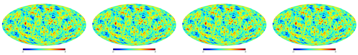
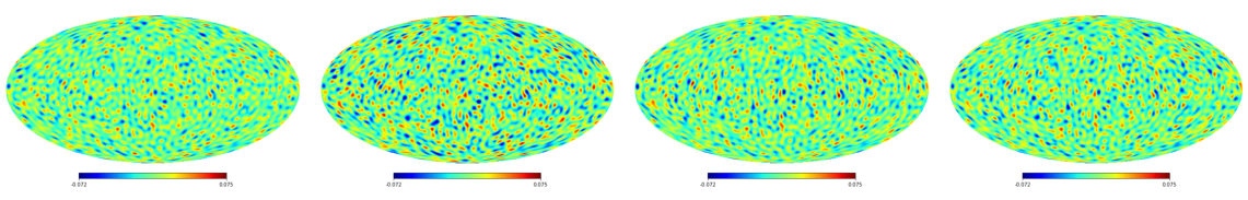
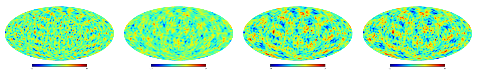
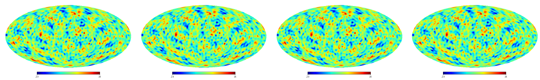
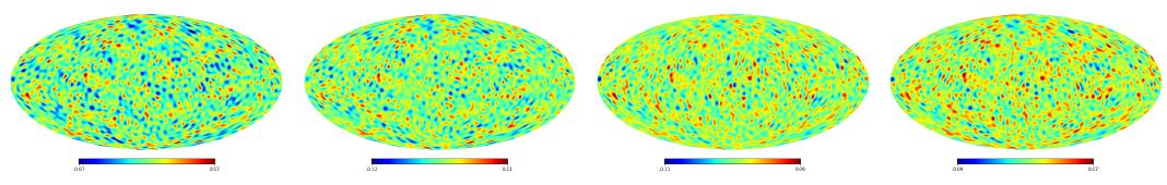
We select some numerical results from Table 1 with and to show the inpainting quality in Figure 2. We observe that our model using Algorithm 4.2 achieves smaller pointwise errors than the optimization model (31) in [32] and group SPGl1 method.
| Algorithm 4.2 | YALL1 | Group SPGl1 | ||||||||||||||
| Mask | RelErr | SNR | RelErr | SNR | RelErr | SNR | ||||||||||
| 7 | 0.0017 | 7 | 7 | 0 | 55.54 | 0.511 | 14 | 6 | 8 | 5.82 | 0.0023 | 12 | 7 | 5 | 52.65 | |
| 11 | 0.0012 | 11 | 11 | 0 | 58.28 | 0.575 | 13 | 9 | 4 | 4.80 | 0.0788 | 23 | 11 | 12 | 56.19 | |
| 19 | 0.0013 | 19 | 19 | 0 | 57.73 | 0.374 | 25 | 17 | 8 | 8.55 | 0.3965 | 29 | 19 | 10 | 46.25 | |
| 7 | 0.0023 | 7 | 7 | 0 | 52.47 | 0.668 | 19 | 7 | 12 | 3.08 | 0.0043 | 17 | 7 | 10 | 47.29 | |
| 11 | 0.0022 | 11 | 11 | 0 | 53.19 | 0.651 | 25 | 11 | 14 | 2.67 | 0.0788 | 32 | 11 | 21 | 22.07 | |
| 19 | 0.0059 | 19 | 19 | 0 | 44.54 | 0.683 | 26 | 19 | 7 | 1.87 | 0.3965 | 33 | 19 | 14 | 8.03 | |
| 7 | 0.0019 | 7 | 7 | 0 | 54.60 | 0.378 | 21 | 7 | 14 | 8.50 | 0.0035 | 16 | 7 | 9 | 49.01 | |
| 11 | 0.0014 | 11 | 11 | 0 | 57.30 | 0.357 | 13 | 11 | 2 | 8.89 | 0.0024 | 26 | 11 | 15 | 52.57 | |
| 19 | 0.0015 | 19 | 19 | 0 | 56.28 | 0.321 | 25 | 19 | 6 | 9.70 | 0.1195 | 34 | 19 | 15 | 18.45 | |
| 7 | 0.0017 | 7 | 7 | 0 | 55.33 | 0.351 | 16 | 6 | 10 | 8.91 | 0.0022 | 12 | 7 | 5 | 52.65 | |
| 11 | 0.0013 | 11 | 11 | 0 | 57.72 | 0.321 | 11 | 9 | 2 | 10.78 | 0.0019 | 23 | 11 | 12 | 54.29 | |
| 19 | 0.0014 | 19 | 19 | 0 | 56.84 | 0.273 | 22 | 17 | 5 | 11.25 | 0.0073 | 32 | 19 | 13 | 42.76 | |
| 6 | 0.0027 | 6 | 6 | 0 | 51.43 | 0.551 | 28 | 5 | 23 | 5.18 | 0.0030 | 13 | 6 | 7 | 50.40 | |
| 16 | 0.0024 | 16 | 16 | 0 | 52.43 | 0.591 | 33 | 13 | 20 | 4.57 | 0.0024 | 33 | 16 | 17 | 52.29 | |
| 26 | 0.0031 | 26 | 26 | 0 | 50.21 | 0.511 | 35 | 23 | 12 | 5.84 | 0.0038 | 37 | 26 | 11 | 48.50 | |
| 6 | 0.0032 | 6 | 6 | 0 | 49.84 | 0.676 | 39 | 6 | 33 | 2.83 | 0.0044 | 15 | 6 | 9 | 47.04 | |
| 16 | 0.0044 | 16 | 16 | 0 | 47.15 | 0.643 | 43 | 16 | 27 | 2.68 | 0.0729 | 45 | 16 | 29 | 22.74 | |
| 26 | 0.0090 | 26 | 26 | 0 | 40.93 | 0.664 | 42 | 26 | 16 | 2.73 | 0.3549 | 47 | 26 | 21 | 8.99 | |
| 6 | 0.0027 | 6 | 6 | 0 | 51.43 | 0.212 | 41 | 6 | 35 | 13.21 | 0.0036 | 14 | 6 | 8 | 48.89 | |
| 16 | 0.0024 | 16 | 16 | 0 | 52.43 | 0.191 | 37 | 16 | 21 | 14.61 | 0.0041 | 38 | 16 | 22 | 47.72 | |
| 26 | 0.0031 | 26 | 26 | 0 | 50.21 | 0.298 | 38 | 26 | 12 | 10.50 | 0.1393 | 48 | 26 | 22 | 17.11 | |
| 6 | 0.0027 | 6 | 6 | 0 | 51.25 | 0.197 | 37 | 6 | 31 | 16.42 | 0.0031 | 14 | 6 | 8 | 50.14 | |
| 16 | 0.0023 | 16 | 16 | 0 | 52.47 | 0.193 | 37 | 16 | 21 | 14.21 | 0.0030 | 32 | 16 | 16 | 50.51 | |
| 26 | 0.0030 | 26 | 26 | 0 | 50.55 | 0.239 | 37 | 25 | 12 | 13.05 | 0.0078 | 44 | 26 | 18 | 42.21 | |
| Algorithm 4.2 | YALL1 | Group SPGl1 | ||||||||||||||
| Mask | RelErr | SNR | RelErr | SNR | RelErr | SNR | ||||||||||
| 7 | 1.90e-4 | 7 | 7 | 0 | 74.42 | 0.551 | 6 | 6 | 0 | 5.83 | 2.88e-4 | 11 | 7 | 4 | 70.78 | |
| 11 | 1.27e-4 | 11 | 11 | 0 | 77.89 | 0.591 | 12 | 9 | 3 | 4.80 | 1.61e-4 | 21 | 11 | 10 | 75.82 | |
| 19 | 1.39e-4 | 19 | 19 | 0 | 77.13 | 0.511 | 25 | 17 | 8 | 8.55 | 0.0035 | 33 | 19 | 14 | 49.18 | |
| 7 | 2.58e-4 | 7 | 7 | 0 | 71.73 | 0.676 | 19 | 19 | 0 | 3.08 | 5.24e-4 | 17 | 7 | 10 | 65.60 | |
| 11 | 2.35e-4 | 11 | 11 | 0 | 72.57 | 0.643 | 21 | 11 | 10 | 2.67 | 0.0859 | 34 | 11 | 23 | 21.32 | |
| 19 | 6.89e-4 | 19 | 19 | 0 | 63.22 | 0.664 | 10 | 7 | 3 | 1.87 | 0.3949 | 33 | 19 | 14 | 8.06 | |
| 7 | 2.08e-4 | 7 | 7 | 0 | 73.60 | 0.212 | 16 | 7 | 9 | 8.50 | 4.05e-4 | 15 | 7 | 8 | 67.84 | |
| 11 | 1.40e-4 | 11 | 11 | 0 | 77.05 | 0.191 | 14 | 11 | 3 | 8.89 | 2.54e-4 | 25 | 11 | 14 | 71.89 | |
| 19 | 1.70e-4 | 19 | 19 | 0 | 75.37 | 0.298 | 21 | 19 | 2 | 9.70 | 0.1172 | 35 | 19 | 16 | 18.62 | |
| 7 | 1.97e-4 | 7 | 7 | 0 | 74.09 | 0.197 | 11 | 6 | 5 | 8.91 | 2.65e-4 | 11 | 7 | 4 | 71.50 | |
| 11 | 1.28e-4 | 11 | 11 | 0 | 77.83 | 0.193 | 9 | 9 | 0 | 10.78 | 1.93e-4 | 22 | 11 | 11 | 74.25 | |
| 19 | 1.56e-4 | 19 | 19 | 0 | 76.13 | 0.239 | 20 | 17 | 3 | 11.26 | 0.0046 | 35 | 19 | 16 | 46.66 | |
| 6 | 2.56e-4 | 6 | 6 | 0 | 71.81 | 0.551 | 13 | 5 | 8 | 5.18 | 3.10e-4 | 11 | 6 | 5 | 70.17 | |
| 16 | 2.15e-4 | 16 | 16 | 0 | 73.32 | 0.591 | 18 | 13 | 5 | 4.57 | 2.67e-4 | 27 | 16 | 11 | 71.44 | |
| 26 | 2.46e-4 | 26 | 26 | 0 | 72.17 | 0.511 | 35 | 22 | 12 | 5.84 | 3.94e-4 | 35 | 26 | 9 | 68.08 | |
| 6 | 3.18e-4 | 6 | 6 | 0 | 69.92 | 0.676 | 16 | 6 | 10 | 2.83 | 4.48e-4 | 16 | 6 | 10 | 66.96 | |
| 16 | 5.09e-4 | 16 | 16 | 0 | 65.85 | 0.643 | 36 | 16 | 20 | 2.68 | 0.0829 | 45 | 16 | 29 | 21.63 | |
| 26 | 9.97e-4 | 26 | 26 | 0 | 60.01 | 0.664 | 32 | 26 | 6 | 2.73 | 0.3562 | 47 | 26 | 21 | 8.98 | |
| 6 | 2.97e-4 | 6 | 6 | 0 | 70.52 | 0.212 | 30 | 6 | 24 | 13.21 | 3.84e-4 | 13 | 6 | 7 | 68.31 | |
| 16 | 2.70e-4 | 16 | 16 | 0 | 71.34 | 0.191 | 24 | 16 | 8 | 14.61 | 4.59e-4 | 34 | 16 | 18 | 66.75 | |
| 26 | 3.28e-4 | 26 | 26 | 0 | 69.65 | 0.298 | 31 | 26 | 5 | 10.50 | 0.1387 | 50 | 26 | 24 | 17.15 | |
| 6 | 2.86e-4 | 6 | 6 | 0 | 70.85 | 0.197 | 23 | 6 | 17 | 16.42 | 3.43e-4 | 11 | 6 | 5 | 69.29 | |
| 16 | 2.56e-4 | 16 | 16 | 0 | 71.82 | 0.193 | 24 | 16 | 8 | 14.21 | 3.27e-4 | 28 | 16 | 12 | 69.69 | |
| 26 | 3.09e-4 | 26 | 26 | 0 | 70.19 | 0.239 | 29 | 25 | 4 | 13.05 | 8.06e-4 | 43 | 26 | 17 | 61.86 | |
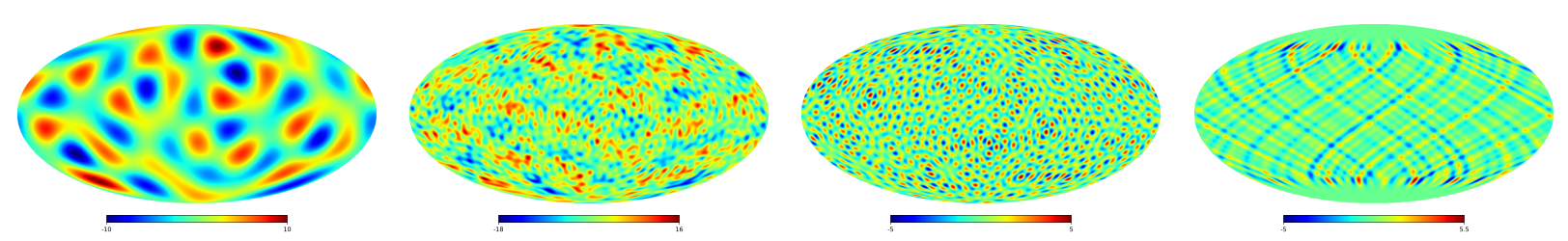
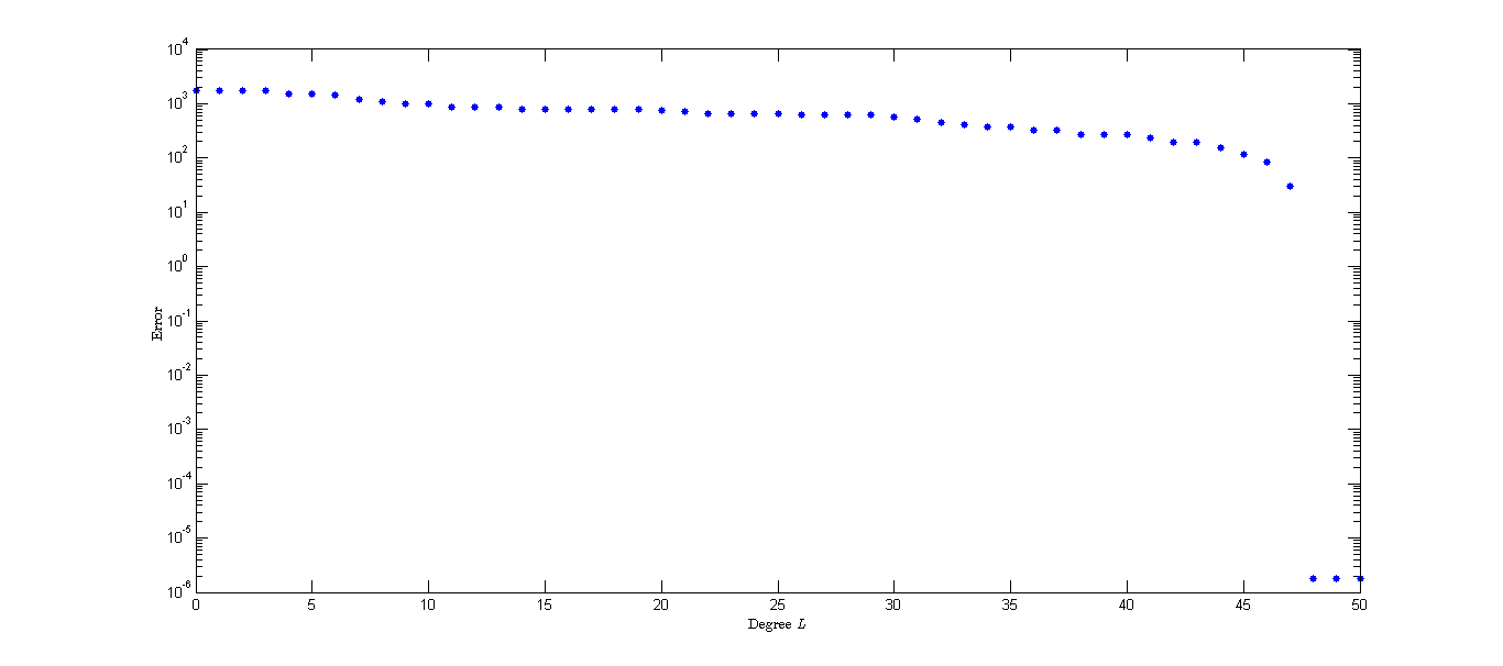
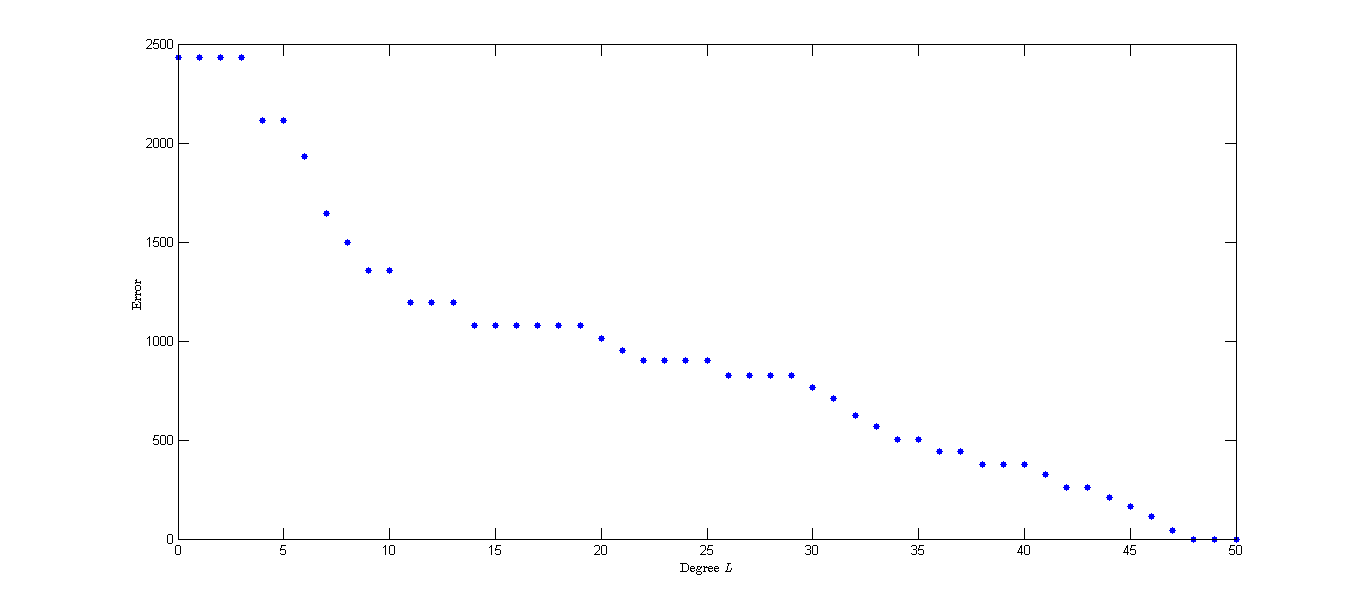
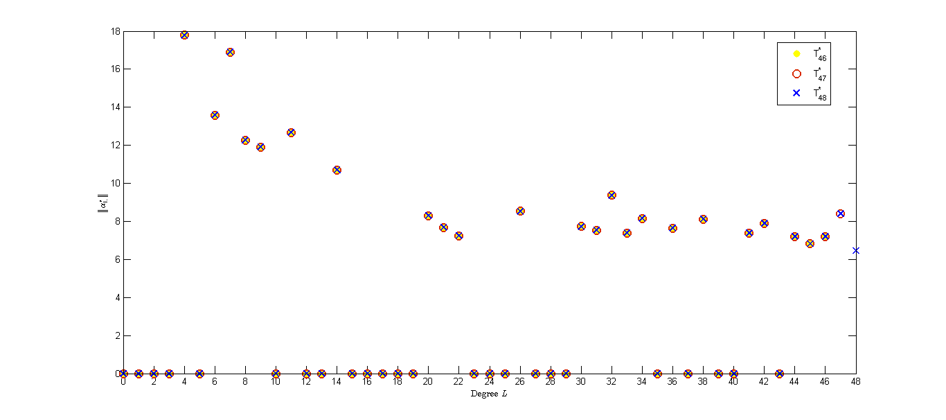
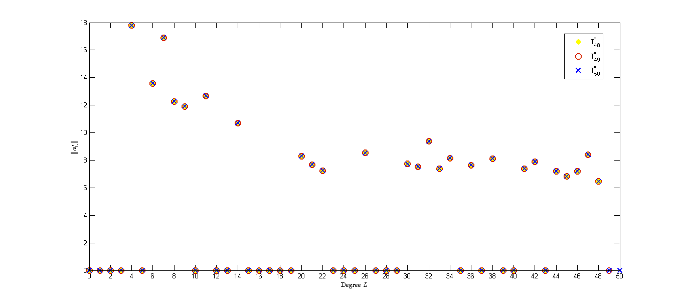
To give some insight for the choice of of the truncated space, we conduct experiments on a random field with different under the noiseless case. We choose the mask and the observed field with degree . In Figure 3(a) we show the approximation error on a logarithmic scale. We can see that the error decreases as increases and the errors are same for . Moreover, and are zero groups of for . From our discussion in Section 2 and Theorem 5.2, we can guess that the value of for (a) is . We plot the error for different in Figure 3(b). We can observe that the error decreases as increases and the errors are zero for due to and . In Figure 3 (c) and (d), we plot the values of of with different to give some insight of the sparsity pattern of .
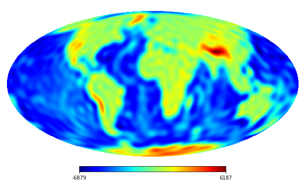
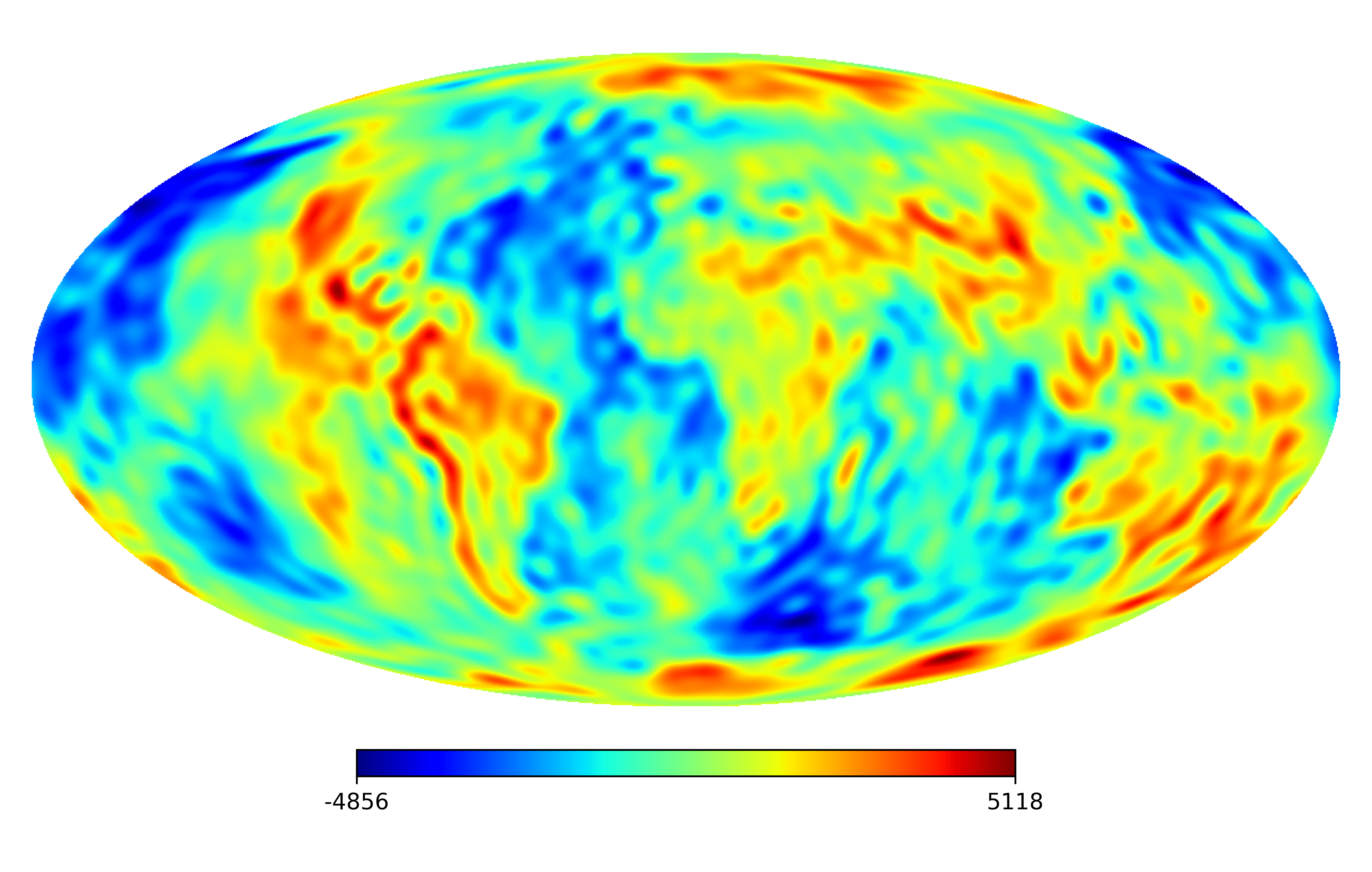
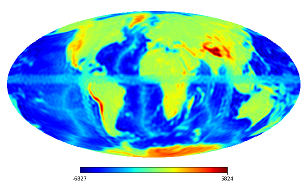
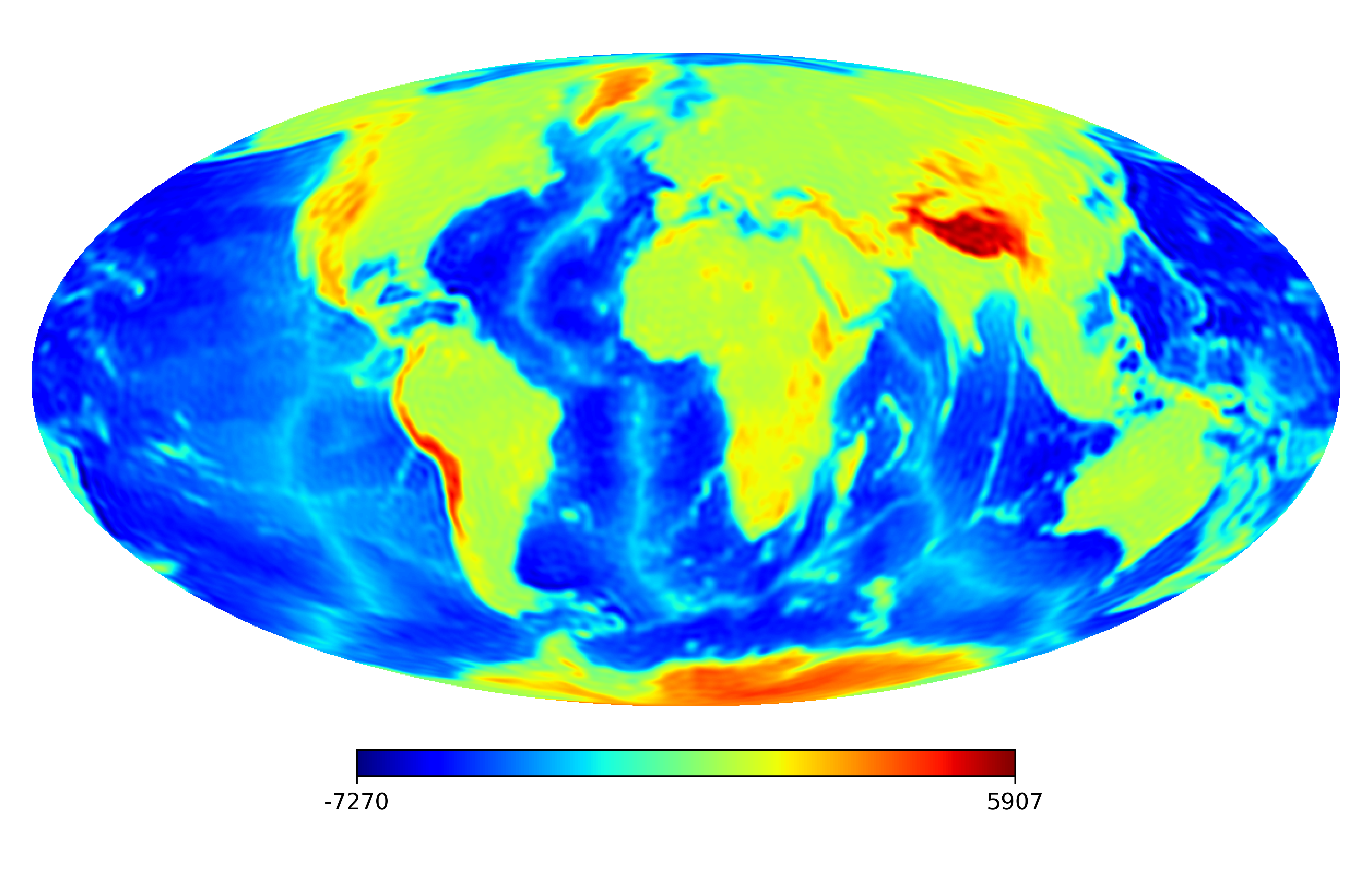
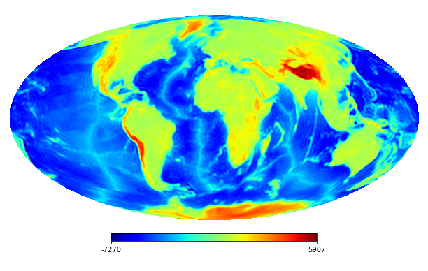
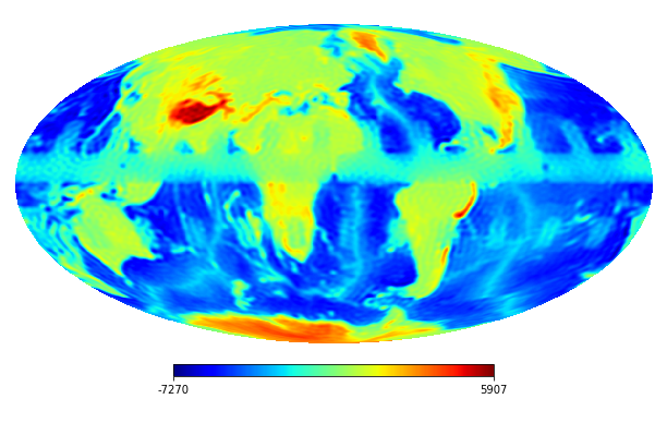
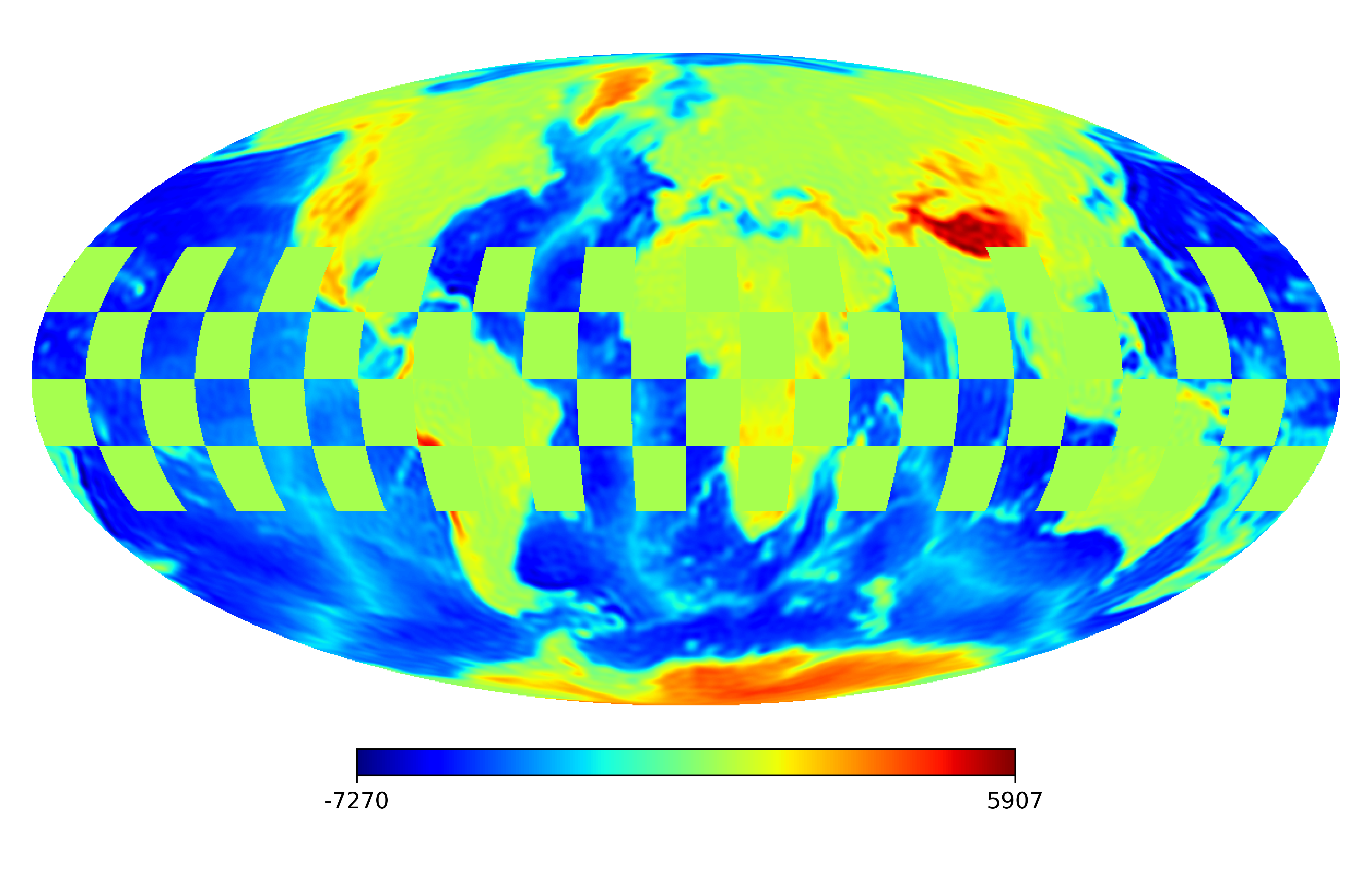
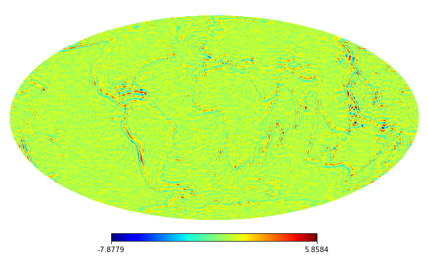
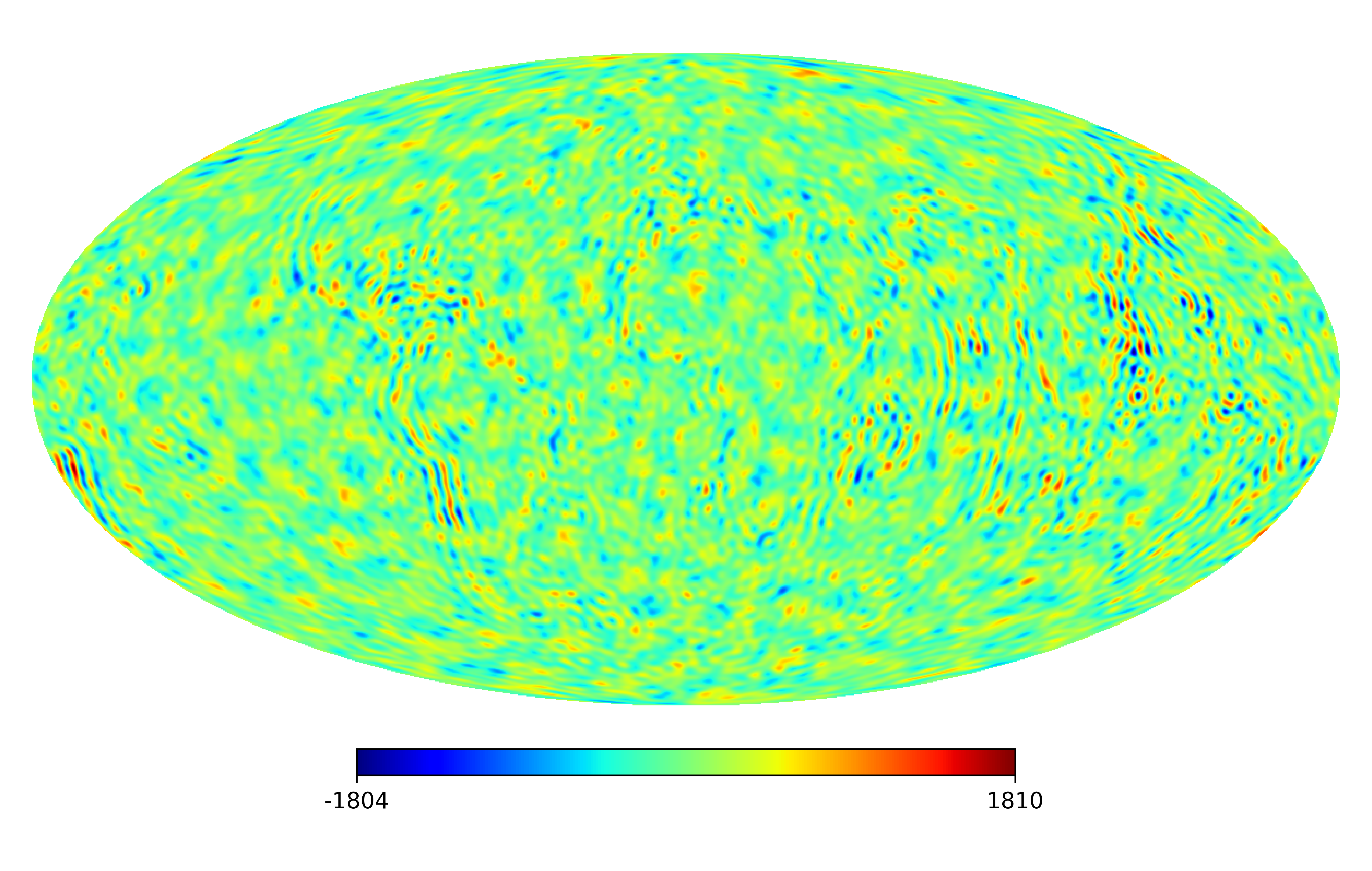
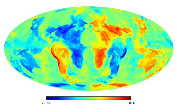
6.2 Real image
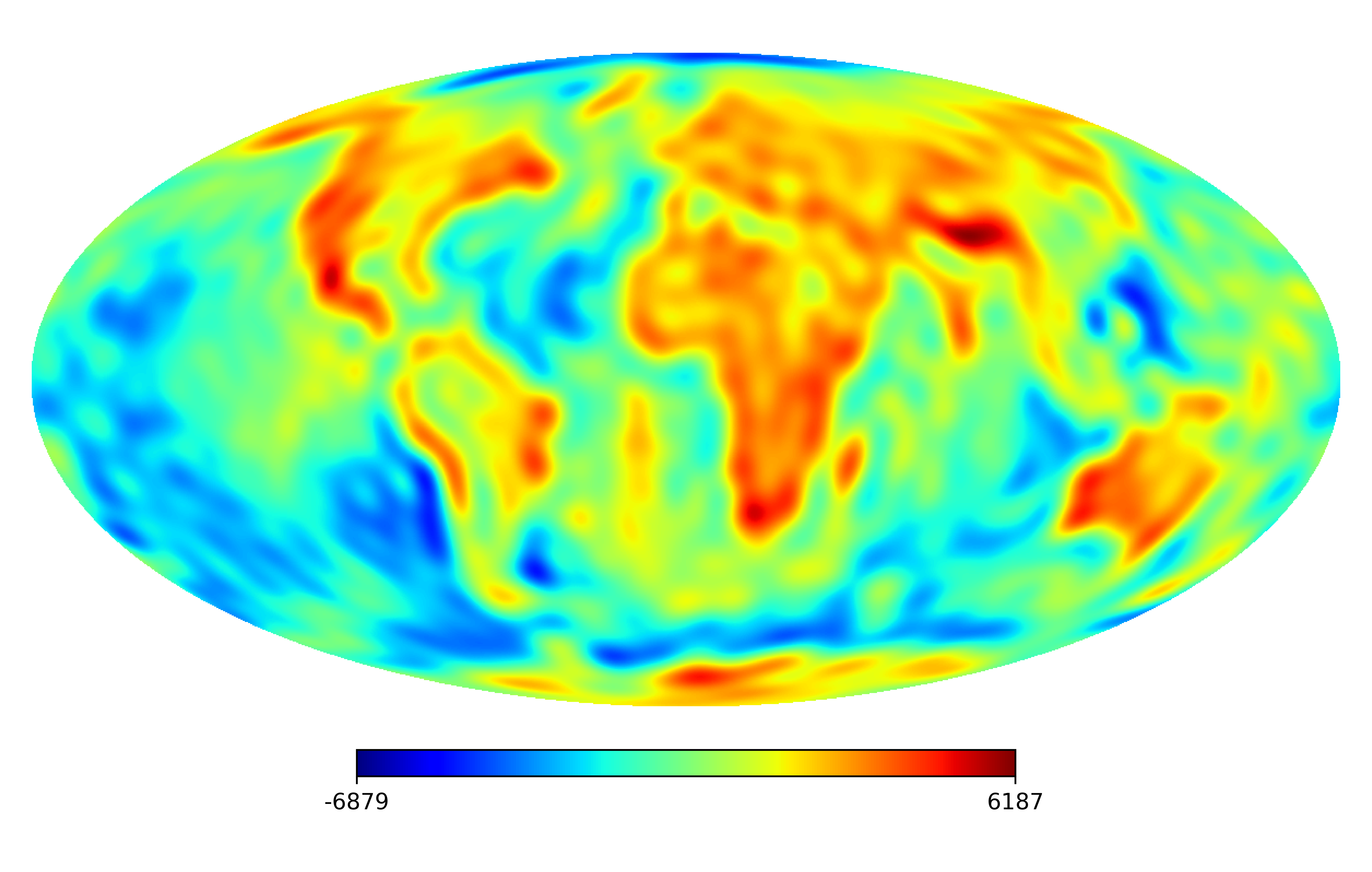
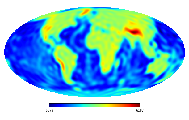
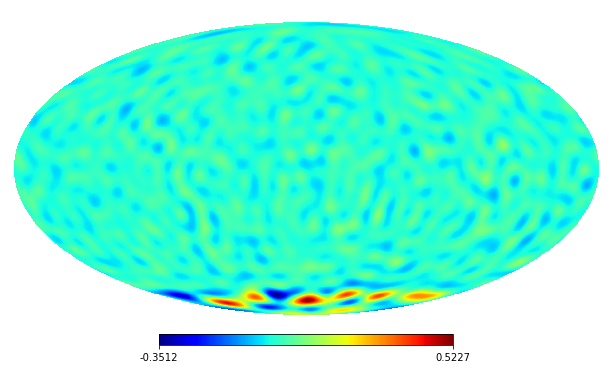
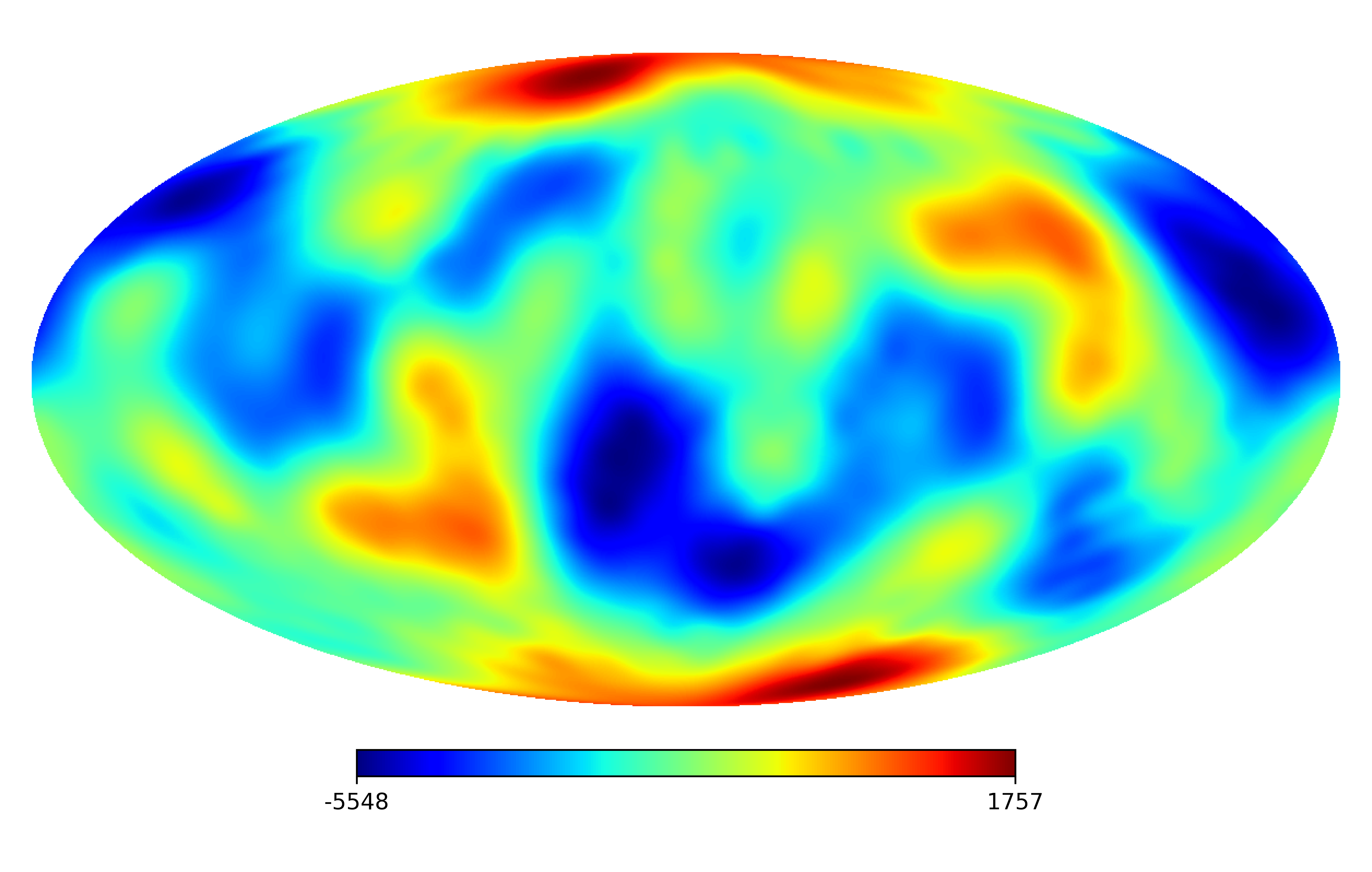
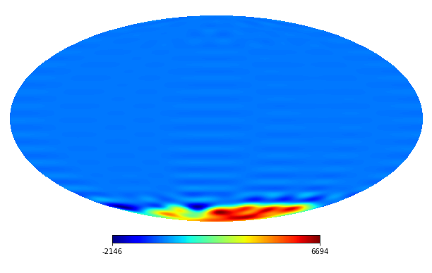
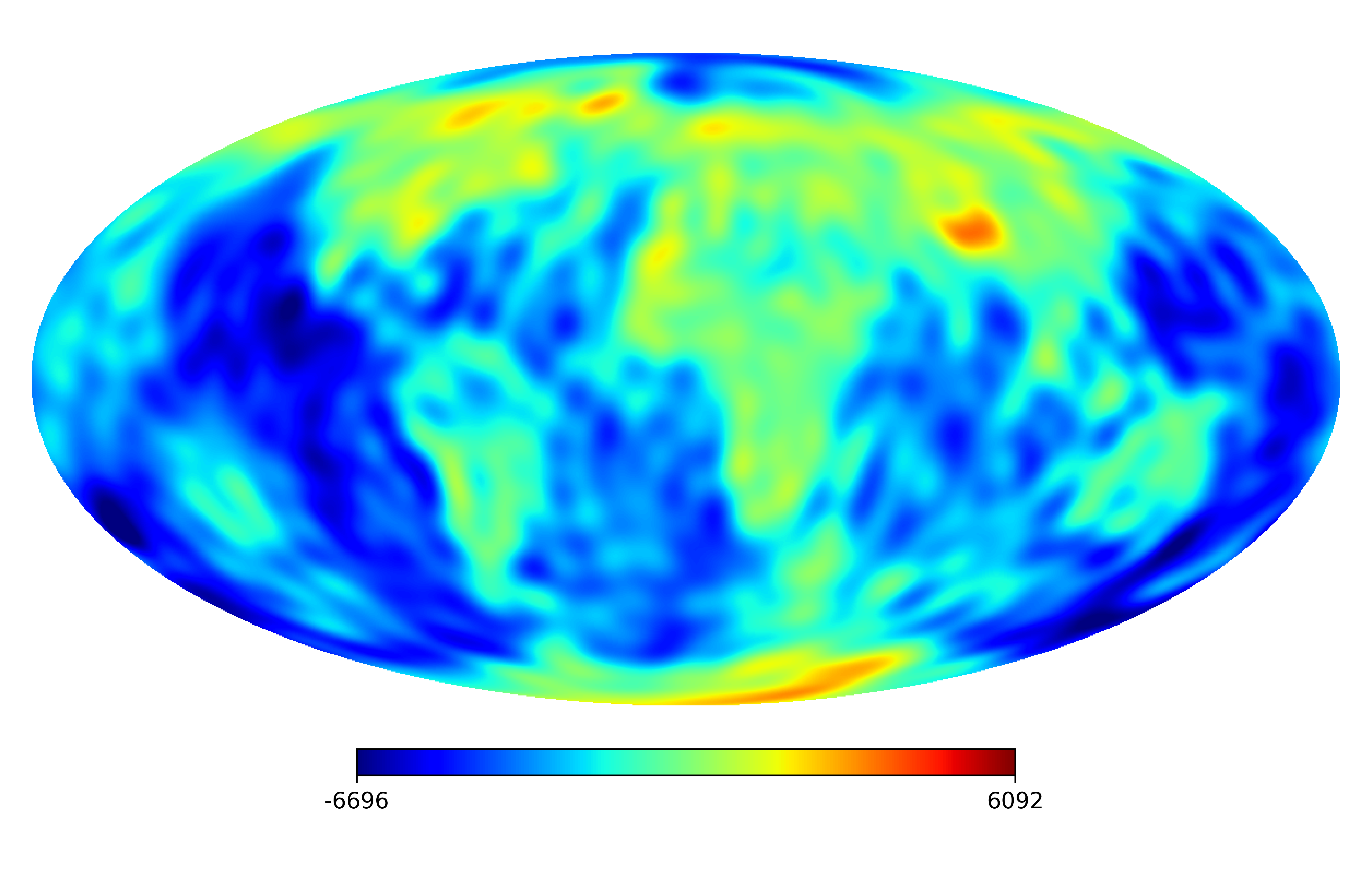
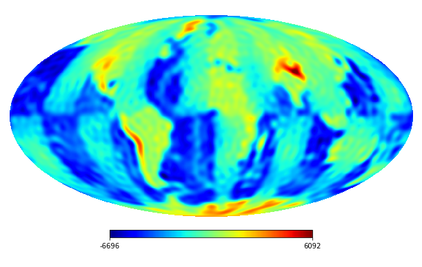
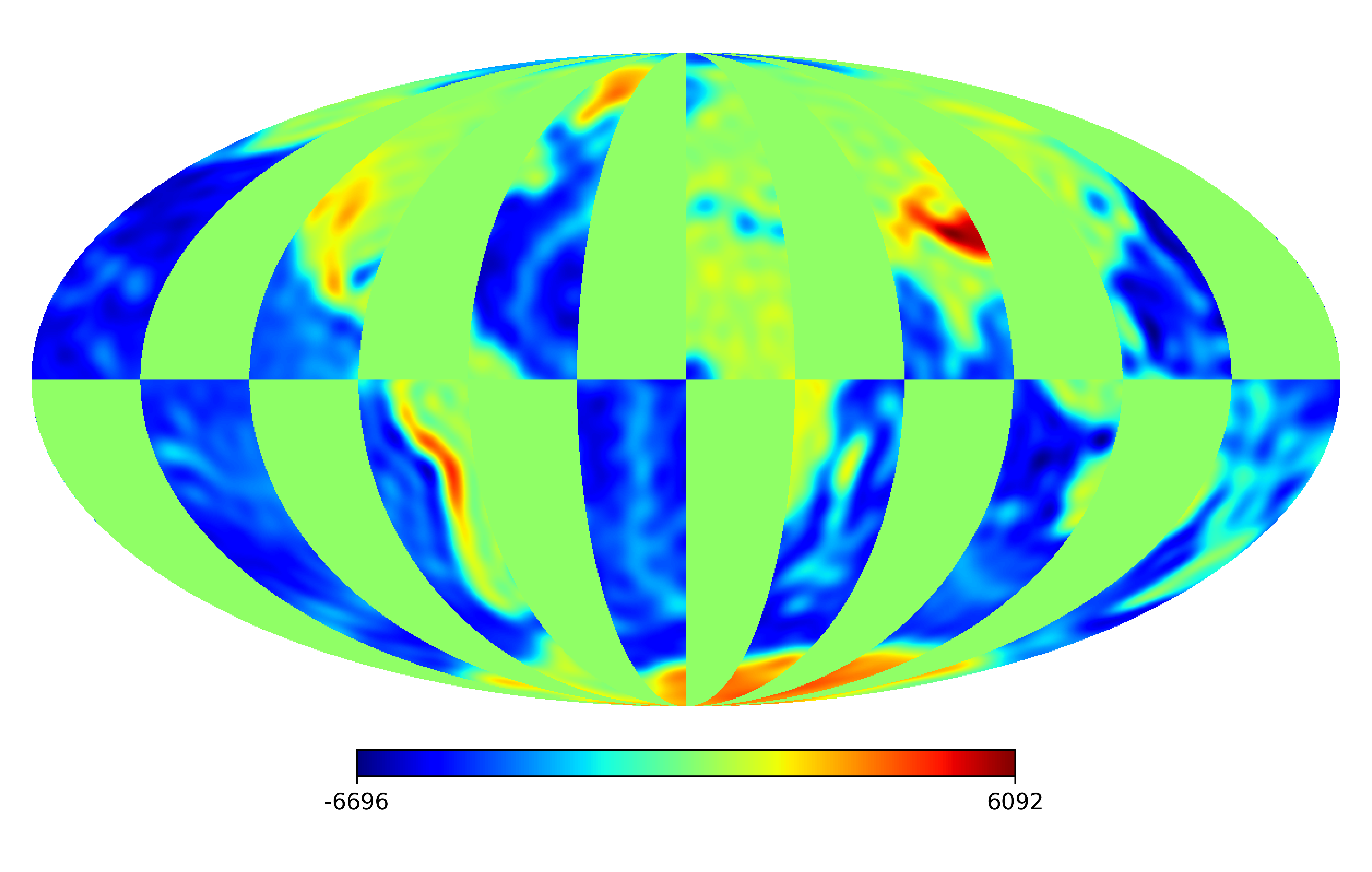
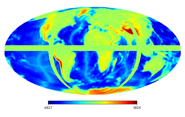
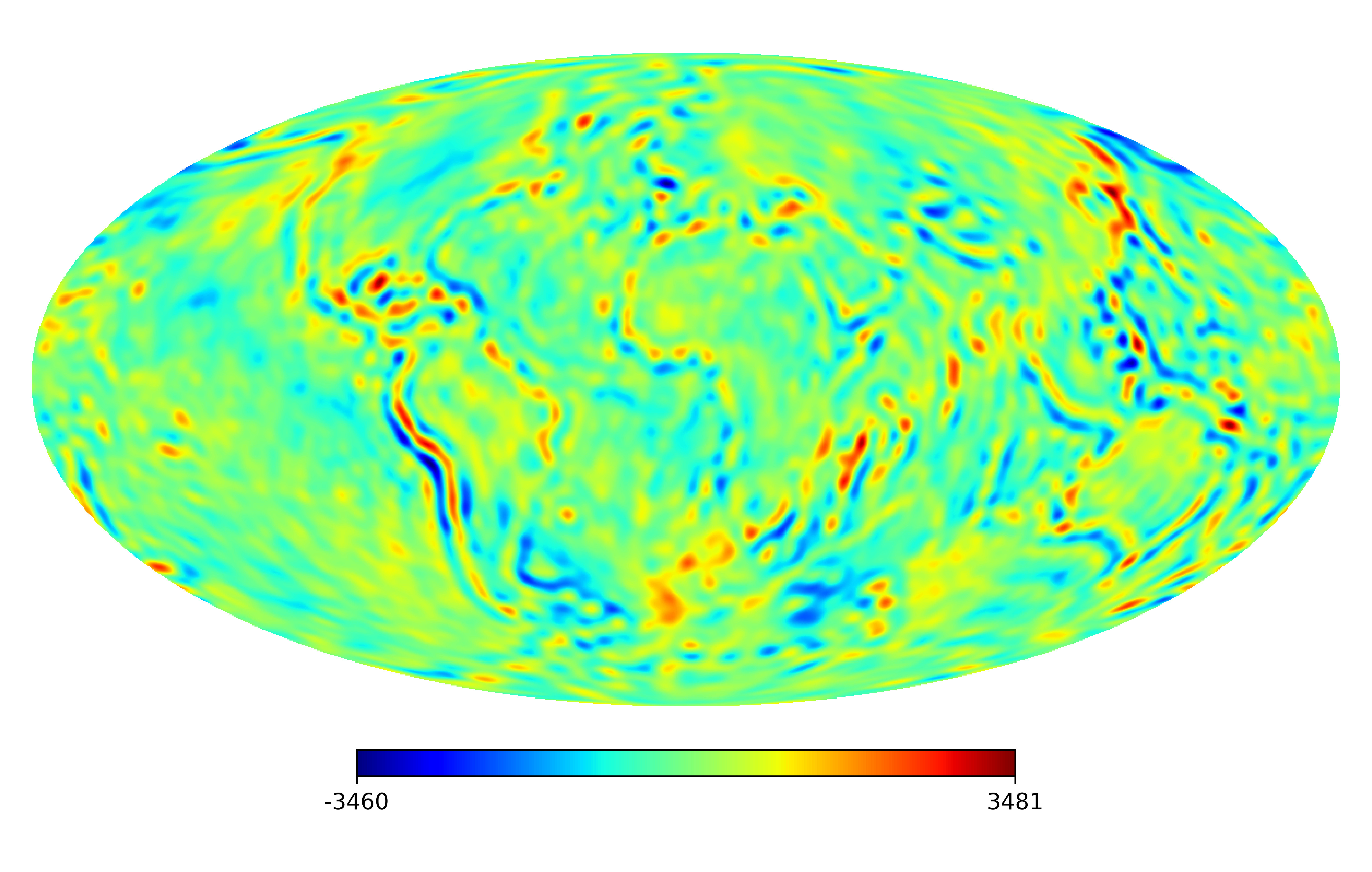
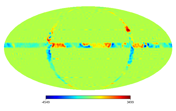
We consider the inpainting of images from Earth topographic data, taken from Earth Gravitational Model (EGM2008) publicly released by the U.S. National Geospatial-Intelligence Agency (NGA) EGM Development Team444http://geoweb.princeton.edu/people/simons/DOTM/Earth.mat. We generate four resolution test images from the Earth topography data which are shown in Figures 5(a), 6(a), 7(a) and 8(a). For each resolution test image we consider a mask which is shown in Figures 5(d), 6(d), 7(d), and 8(d) respectively. For all the images we set . The recovered images and pointwise errors are presented in Figures 5, 6, 7 and 8. We can see that model (2.5) using Algorithm 4.2 yields higher quality images with smaller pointwise errors and higher SNR values than the optimization model (31) in [32] and the group SPGl1 method under different resolutions.


7 Conclusion
In this paper, we propose a constrained group sparse optimization model (1.6) for the inpainting of random fields on the unit sphere with unique continuation property. Based on the K-L expansion, we rewrite the constraint in (1.6) in a discrete form and derive an equivalence formulation (2.2) of problem (1.6). For problem (2.2), we derive a lower bound (2.4) for the norm of nonzero groups of its scaled KKT points. We show that problem (2.2) is equivalent to the finite-dimensional problem (2.5). For this finite-dimensional problem (2.5) and its penalty problem (2.6), we prove the exact penalization in terms of local minimizers and -minimizers. Moreover, we propose a smoothing penalty algorithm for solving problem (2.5) and prove its convergence. We also present the approximation error of the inpainted random field represented by the scaled KKT point in the space . Finally, we present numerical results on band-limited random fields on the sphere and the images from Earth topographic data to show the promising performance of our model by using the smoothing penalty algorithm.
References
- [1] P. Abrial, Y. Moudden, J.L. Starck, B. Afeyan, J. Bobin, J. Fadili, and M.K. Nguyen. Morphological component analysis and inpainting on the sphere: application in physics and astrophysics. J. Fourier Anal. Appl., 13(6):729–748, 2007.
- [2] S. Axler, P. Bourdon, and R. Wade. Harmonic Function Theory, volume 137. Springer Science & Business Media, 2013.
- [3] Amir Beck and Nadav Hallak. Optimization problems involving group sparsity terms. Math. Program., 178(1):39–67, 2019.
- [4] D.H. Brandwood. A complex gradient operator and its application in adaptive array theory. IEE Proceedings H - Microwaves, Optics and Antennas, 130(1):11–16, 1983.
- [5] P. Cabella and D. Marinucci. Statistical challenges in the analysis of cosmic microwave background radiation. Ann. Appl. Stat., 3:61–95, 2009.
- [6] V. Cammarota and D. Marinucci. The stochastic properties of -regularized spherical Gaussian fields. Appl. Comput. Harmon. Anal., 38(2):262–283, 2015.
- [7] X. Chen. Smoothing methods for nonsmooth, nonconvex minimization. Math. Program., 134(1):71–99, 2012.
- [8] X. Chen, Z. Lu, and T.K. Pong. Penalty methods for a class of non-Lipschitz optimization problems. SIAM J. Optim., 26(3):1465–1492, 2016.
- [9] X. Chen and R.S. Womersley. Spherical designs and nonconvex minimization for recovery of sparse signals on the sphere. SIAM J. Imaging Sci., 11(2):1390–1415, 2018.
- [10] X. Chen, F. Xu, and Y. Ye. Lower bound theory of nonzero entries in solutions of - minimization. SIAM J. Sci. Comput., 32(5):2832–2852, 2010.
- [11] Xiaojun Chen and Ph L Toint. High-order evaluation complexity for convexly-constrained optimization with non-lipschitzian group sparsity terms. Math. Program., 187(1):47–78, 2021.
- [12] P.E. Creasey and A. Lang. Fast generation of isotropic Gaussian random fields on the sphere. Monte Carlo Methods Appl., 24(1):1–11, 2018.
- [13] S.M. Feeney, D. Marinucci, J.D. McEwen, H.V. Peiris, B.D. Wandelt, and V. Cammarota. Sparse inpainting and isotropy. J. Cosmol. Astropart. Phys., 2014(1):050, 2014.
- [14] Q.T. Le Gia, I.H. Sloan, R.S. Womersley, and Y.G. Wang. Sparse isotropic regularization for spherical harmonic representations of random fields on the sphere. Appl. Comput. Harmon. Anal., 49:257–278, 2019.
- [15] K.M. Górski, E. Hivon, A.J. Banday, B.D. Wandelt, F.K. Hansen, M. Reinecke, and M. Bartelmann. Healpix: a framework for high-resolution discretization and fast analysis of data distributed on the sphere. Astrophys. J., 622(2):759–771, 2005.
- [16] E. Hille. Analytic Function Theory, volume 2. American Mathematical Soc., 2005.
- [17] Jian Huang, Shuange Ma, Huiliang Xie, and Cun-Hui Zhang. A group bridge approach for variable selection. Biometrika, 96(2):339–355, 2009.
- [18] Junzhou Huang and Tong Zhang. The benefit of group sparsity. Ann. Statist., 38(4):1978–2004, 2010.
- [19] V. Isakov. Inverse Problems for Partial Differential Equations, volume 127. Springer, 2006.
- [20] J. Jeong, M. Jun, and M. Genton. Spherical process models for global spatial statistics. Stat. Sci., 32(4):501–513, 2017.
- [21] Z. Khalid, R.A. Kennedy, and J.D. McEwen. An optimal-dimensionality sampling scheme on the sphere with fast spherical harmonic transforms. IEEE Trans. Signal Process., 62(17):4597–4610, 2014.
- [22] K. Kreutz-Delgado. The complex gradient operator and the CR-calculus. arXiv:0906.4835, 2009.
- [23] A. Lang and C. Schwab. Isotropic Gaussian random fields on the sphere: regularity, fast simulation and stochastic partial differential equations. Ann. Appl. Probab., 25(6):3047–3094, 2015.
- [24] C. Li and X. Chen. Isotropic non-Lipschitz regularization for sparse representations of random fields on the sphere. Math. Comp., 91:219–243, 2022.
- [25] D. Marinucci and G. Peccati. Random Fields on the Sphere: Representations, Limit Theorems and Cosmological Applications. Cambridge University Press, Cambridge, 2011.
- [26] H.S. Oh and T.H. Li. Estimation of global temperature fields from scattered observations by a spherical-wavelet-based spatially adaptive method. J. R. Statist. Soc. B, 66(1):221–238, 2004.
- [27] Lili Pan and Xiaojun Chen. Group sparse optimization for images recovery using capped folded concave functions. SIAM J. Imaging Sci., 14(1):1–25, 2021.
- [28] E. Porcu, A. Alegria, and R. Furrer. Modeling temporally evolving and spatially globally dependent data. Int. Stat. Rev., 86(2):344–377, 2018.
- [29] R.T. Rockafellar and R.J-B Wets. Variational Analysis. Springer Science & Business Media, 2009.
- [30] J.L. Starck, M. Fadili, and A. Rassat. Low- CMB analysis and inpainting. Astron. Astrophys., 550:A15, 2013.
- [31] M.L. Stein. Spatial variation of total column ozone on a global scale. Ann. Appl. Stat., 1(1):191–210, 2007.
- [32] C.G.R. Wallis, Y. Wiaux, and J.D. McEwen. Sparse image reconstruction on the sphere: analysis and synthesis. IEEE Trans. Image Process., 26(11):5176–5187, 2017.
- [33] J. Yang and Y. Zhang. Alternating direction algorithms for -problems in compressive sensing. SIAM J. Sci. Comput., 33(1):250–278, 2011.
- [34] Ming Yuan and Yi Lin. Model selection and estimation in regression with grouped variables. J. R. Stat. Soc. B, 68(1):49–67, 2006.
Appendix A. Unique continuation property
In this Appendix, we give details about the unique continuation property of a class of fields with spherical harmonic representations.
Let be a positive constant for some , be an open ball centered at of radius . Let
| (.1) |
be a class of fields with spherical harmonic representations and coefficients belong to . Then we show that any has the unique continuation property. Let be given by
where .
Lemma 3.
If , then .
Proof.
Since and , there exists an integer such that for any , Then, we obtain, for any , which implies that . Thus, This completes the proof. ∎
Lemma 4.
is real analytic in .
Proof.
Let , where . By definition of harmonic functions [2], , , are harmonic functions on . Then we obtain that , are harmonics functions on . Moreover, for any and ,
where the first inequality follows from Cauchy-Schwarz inequality, the second equality follows from addition theorem of spherical harmonics and the last inequality follows from and .
By Lemma 3, , then for any , there exists such that for any , we have that for any ,
Thus, the sequence of harmonic functions converges uniformly to on .
Lemma 5.
For any , if there exists a sequence of distinct points , with at least one limit point in , and if , , then on .
Proof.
Now we present the unique continuation property of any .
Theorem 8.
For any , if on , then on .
Proof.
Since the coefficients and has an open subset, we know from Lemma 5 that if on then on . ∎
By Parseval’s theorem, for any , we have , which implies that if and only if . Hence, we can claim that for any , if and only if .
Appendix B. Wirtinger gradient
In this appendix, we briefly introduce the Wirtinger gradient of real-valued functions with complex variables. For more details about Wirtinger calculus, we refer to [4, 22, 24].
Let be a real-valued function of a vector of complex variables , which can be written as , that is . Let , where . We say is Wirtinger differentiable, if is differentiable with respect to and , respectively. Following [4, 22], under the conjugate coordinates , the Wirtinger gradient of at is
where , Since is real-valued, . Thus,
We say is a stationary point of if it satisfies
It is easy to verify that the Wirtinger gradient of , , is and is a stationary point of if .