Greybody factors for higher-dimensional non-commutative geometry inspired black holes
Abstract
Greybody factors are computed for massless fields of spin 0, 1/2, 1, and 2 emitted from higher-dimensional non-commutative geometry inspired black holes. Short-range potentials are used with path-ordered matrix exponentials to numerically calculate transmission coefficients. The resulting absorption cross sections and emission spectra are computed on the brane and compared with the higher-dimensional Schwarzschild-Tangherlini black hole. A non-commutative black hole at its maximum temperature in seven extra dimensions will radiate a particle flux and power of 0.72-0.81 and 0.75-0.81, respectively, times lower than a Schwarzschild-Tangherlini black hole of the same temperature. A non-commutative black hole at its maximum temperature in seven extra dimensions will radiate a particle flux and power of 0.64-0.72 and 0.60-0.64, respectively, times lower than a Schwarzschild-Tangherlini black hole of the same mass.
,
Keywords: greybody factors, black holes, extra dimensions, quantum gravity, non-commutative geometry
1 Introduction
Non-commutative (NC) space-time geometry has allowed insight into the quantum nature of gravity. Within the effective theory for NC black holes, the point-like sources in the energy-momentum tensor, that are normally represented by Dirac delta functions of position, are replaced by Gaussian smeared matter distributions of width . Effective theories for non-commutativity have enable calculations of black hole properties distinctly different from those of classical gravity. The NC black hole has a finite maximum temperature. A minimum mass and horizon radius exist at which the temperature is zero and the heat capacity vanishes which may terminate Hawking evaporation. These properties are in clear contradistinction to the classical black hole with temperature becoming infinite as it approaches zero mass and horizon radius.
Many studies have elucidated the nature of NC geometry inspired black holes but little attention has been devoted to the calculation of greybody factors and their subsequent use in studying absorption cross sections, and particle and energy spectra. Models for NC geometry inspired chargeless, non-rotating black holes were developed by Nicolini, Smailagic and Spallucci [1]. The model was extended to the case of charge in four dimensions [2], generalized to higher dimensions by Rizzo [3], and then to charge in higher dimensions [4]. A review of the developments can be found in Ref. [5]. The Hawking effect and other thermodynamic aspects of NC black holes have been studies in Ref. [6, 7, 8]. Phenomenological considerations for searches with the Large Hadron Collider (LHC) experiments appeared in Ref. [9]. Graybody factor calculations for massless scalar emission were presented in Ref. [10].
The aim of this paper is to present the emission spectra from non-rotating NC inspired black holes in higher dimensions for massless fields of spin 0, 1/2, 1, and 2. The results are compared with the higher-dimensional Schwarzschild-Tangherlini (ST) black hole. One of our goals is to separate the temperature characteristics from the transmission factors in the comparison of emission by performing calculations of the graybody factors for different black hole masses.
Throughout, we will work in units of , and use the PDG [11] definition for the higher-dimensional ADD Planck scale . Note that is often used in the literature. When TeV is taken, the value of will be more than four times beyond the current experimental lower bounds on for , and ruled out for and 2 extra dimensions. To allow comparisons with the literature, we have taken the common values of . For , the units are TeV and m, and for , and units can be chosen as TeV and fm.
2 Non-commutative geometry inspired black holes
A nice review of NC geometry inspired black holes already exists [5]. We will only present the mathematical results used here. The component of the NC inspired metric is
| (1) |
where
| (2) |
and is the normalized lower-incomplete gamma function
| (3) |
The symbols are for the mass of the black hole and for the radial distance from the center of the black hole.
For the effective potentials to be discussed soon, we will also require the derivative of the metric function with respect to :
| (4) |
These expressions reduce to the higher-dimensional commutative forms in the limit or .
The horizon radius for non-commutative inspired black holes is given by
| (5) |
We are unaware of a closed form solution to this equation and so have solved it numerically for . In the commutative limit, the horizon reduces to the usual higher-dimensional ST case, which can be written as
| (6) |
Depending on the context, will be used to refer to both NC and ST black hole horizon radii.
For given , , , and , there can be one, two, or no horizon. For reasons related to positive temperature given later, only the outer horizon radius is relevant to the work presented here. Figure 1 shows for the case of a single event horizon for , , and , and a comparison with the ST black hole.
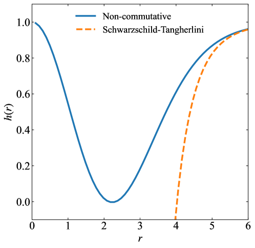
Because there is a minimum mass, there are masses below which the black hole will not form, and above the minimum mass the horizon radius is double valued. As the mass increases, the inner horizon radius shrinks to zero, while the outer horizon radius approaches the commutative value. The situation thus depicted in Figure 1 represents the minimum mass case in which the values of the horizon radii for NC and ST black holes are maximally different. This will be a useful condition when considering maximum differences in the transmission coefficients between NC and ST black holes.
3 Transmission coefficients
Hawking radiation from black holes is typically studied by examining the response to perturbations. Hence, understanding modifications of Hawking radiation due to NC geometry requires one to solve the equations of motion for various spin perturbations on the NC inspired black hole metric.
The Teukolsky equation describes spin 0, 1/2, 1, and 2 field perturbations in the background metric due to the black hole [12, 13, 14]. The partial differential equations can be separated. The angular equation can be numerically solved to obtain the energy eigenvalues or separation constant. The energy eigenvalues are then used in the radial equation. The radial equation can be solve to find transmission coefficients for fields emitted from the black hole horizon. The transmission coefficients describe the probability that a particle, generated by quantum fluctuations at the horizon of a black hole, escapes to spatial infinity.
The Teukolsky radial equation can be numerically solved directly, but the convergence of the solution at the integration boundaries is not clear. The difficulty with the radial equation in the context of a scattering problem is that the first order radial derivatives create complex terms which have a behaviour at infinity. This can eventually lead to problems in the numerical computations.
Another approach uses a Chandrasekhar transformation [15] to cast the radial equation into an effective Schrödinger equation with a short-range barrier potential different for each spin field, allowing a more careful numerical treatment. The equation takes the form
| (7) |
where is the spin of the field and a generalized tortoise coordinate. We are now faced with a potential-barrier problem.
The purpose of this transformation is that the potentials are now short-ranged. They vanish faster than which is advantageous for numerical computations. It should be noted that these potentials contain a dependence on through the connection coefficient to the angular equation. Working with real-valued potentials has benefits.
Arbey et al. [16] have derived general potentials for spherical symmetric metrics for different spins of massless fields. The effective potentials seen by , and 2 massless fields can be written as
| (8a) | |||||
| (8b) | |||||
| (8c) | |||||
| (8d) | |||||
where , , , and is the angular momentum quantum number.
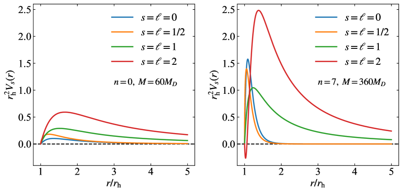
For spin 1/2, one must take the positive sign in Eq. (8b) to get a positive potential for all . For the spin-2 case, for high and , it is possible to get a negative potential. We will discuss this further below when describing absorption cross section results. These potentials differ from those in Ref. [16] in that they are missing a factor in the second term of Eq. (5.1d), and Eq. (5.9c) should have a first constant of 4 rather than 2 in the second term and a constant of 3 rather than 1 in the last term.
Figure 2 shows two representative cases for the NC black hole potentials with for spin 0, 1/2, 1, and 2; the case of is shown.
The Schrödinger Eq. (7) is in the tortoise coordinate while the potential is in ; or one can view . The relationship between the coordinates is defined by
| (8i) |
We note that at , , and as , .
One thus needs to solve differential Eq. (8i) for and also invert it to obtain . While the result is well known for the four-dimensional Schwarzschild metric it is less apparent for others. Analytic expressions exist for for the higher dimensional ST case but we are unaware of such analytic expressions for the NC case. We have thus numerically integrated Eq. (8i). For the initial condition, we take for a very large value (approximating ), and integrate backwards. The procedure has been validated in the ST case by comparing the numerical integrations with the analytic results. The analytic formulae are taken from Ref. [17], to which we have added the case:
| (8j) |
where . We note that Eq. (A5) in Ref. [17] is missing an essential negative sign under the square-root for the first .
We integrate the tortoise equation using a variable step size over the range , where . To obtain the inverse relation for in terms of , we have integrated the tortoise equation and numerically inverted it using linear interpolation.
Gray and Visser [18] showed that the Bogoliubov coefficients relating incoming and outgoing waves on a potential barrier can be directly obtained from the following path-ordered exponential
| (8k) |
where is a path-ordering operator. Using the product calculus definition of path-ordered integrals, they compute the Bogoliubov coefficients via the product integrals
| (8l) |
where is the identity matrix and is the transfer matrix given by
| (8m) |
The product integral can be approximated numerically by
| (8n) |
where and is the step size. We have taken .
The transmission probabilities are related to the Bogoliubov coefficients by
| (8o) |
By using this procedure, one does not actually solve numerically a differential equation. The problem becomes one of performing a single numerical integral, Eq. (8n).
4 Hawking emission
In studying Hawking emission from NC geometry inspired black holes, we consider the following. The absorption cross section is an observable acting as an effective area representing the likelihood of a particle to be scattered by the black hole:
| (8p) |
where are transmission coefficients, greybody factors, for angular momentum mode , and is a multiplicity factor for the azimuthal modes in spherical geometry.
One of the most interesting aspects of NC inspired black holes is their temperature properties. The temperature in terms of the horizon radius is given by
| (8q) |
The quantity in square brackets modifies the usual higher-dimensional commutative form. In addition, since has been modified, it also leads to temperature differences. Since the inner horizon radius corresponds to negative temperature, we only considered the outer radius. Figure 3 shows the temperature versus horizon radius for NC black holes with . The temperature vanishes at the minimum mass and there is a maximum temperature. Also shown for comparison are the usual temperatures for ST black holes.
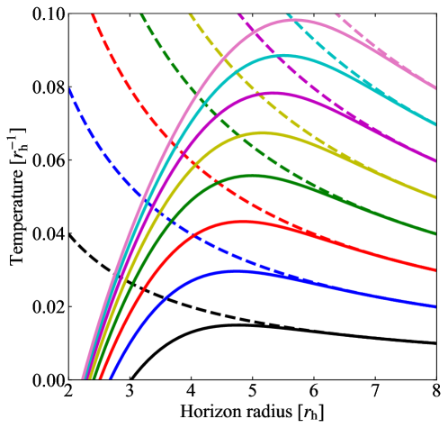
Of interest to us will be the NC black hole maximum temperature and mass at which the maximum temperature occurs. In addition, we will use values of the ST black hole mass at which the temperature is the same as the NC black hole maximum temperature. These values are shown in Table 1.
-
0 1 2 3 4 5 6 7 0.015 0.030 0.043 0.056 0.067 0.078 0.089 0.098 60.47 108.3 157.5 204.9 249.1 289.4 325.6 357.7 66.95 136.0 224.8 332.0 456.4 597.0 753.0 923.7
We now introduce the main physical variables that can be formulated using the transmission coefficients. The number of particles emitted per unit time and per unit frequency is
| (8r) |
The energy emitted per unit time (or power) and per unit frequency is
| (8s) |
We acknowledge a damping factor that was developed in Ref.[10] that multiplies Eq. (8r) and Eq. (8s). Including this factor gives a sub-dominate effect [10] which is not particularly relevant to our discussion and will be ignored.
The black body radiation leaving the horizon sees an effective potential barrier due to the geometry of the space-time surrounding the black hole. The potential barrier attenuates the radiation such that an observer at spatial infinity away from the black hole will measure a different emission spectrum than the one at the horizon by a factor called the greybody factor. Thus the grey body factor represents the fraction of the black body emission which penetrates through the potential barrier and escapes to spatial infinity. The expressions for absorption cross section Eq. (8p) and emission rates Eq. (8r) and Eq. (8s) are only applicable to radiation on the brane.
5 Results
We present calculations of transmission coefficients, absorption cross sections, and spectra for spin 0, 1/2, 1, and 2 fields. We have validated the method by comparing with well known results for four dimensional Schwarzschild and Kerr black holes, as well as the ST black holes [19, 20] that we use for comparison with the NC results.
The model of NC geometry inspired black holes in higher dimensions has three unknown parameters , , and . Typically we present results for each extra dimension . Usually it is necessary to fix the other two parameters. One possibility for fixing the parameters is to be guided by experimental constraints. Updating the approach taken in Ref. [9] (see the Appendix) restricts the values of that can be probed from 0.25 to 0.98, different for each number of extra dimensions. The allowed range in for any given number of extra dimensions is severely restricted.
Calculations using values of begin to probe the details of the matter smearing distribution and become model dependent. However, the primary goal in this paper is to study the differences in Hawking emission from NC and ST black holes so we choose the usual condition . This implies that our phenomenological predictions will not have particular consequence for the physics at the LHC.
5.1 Transmission coefficients
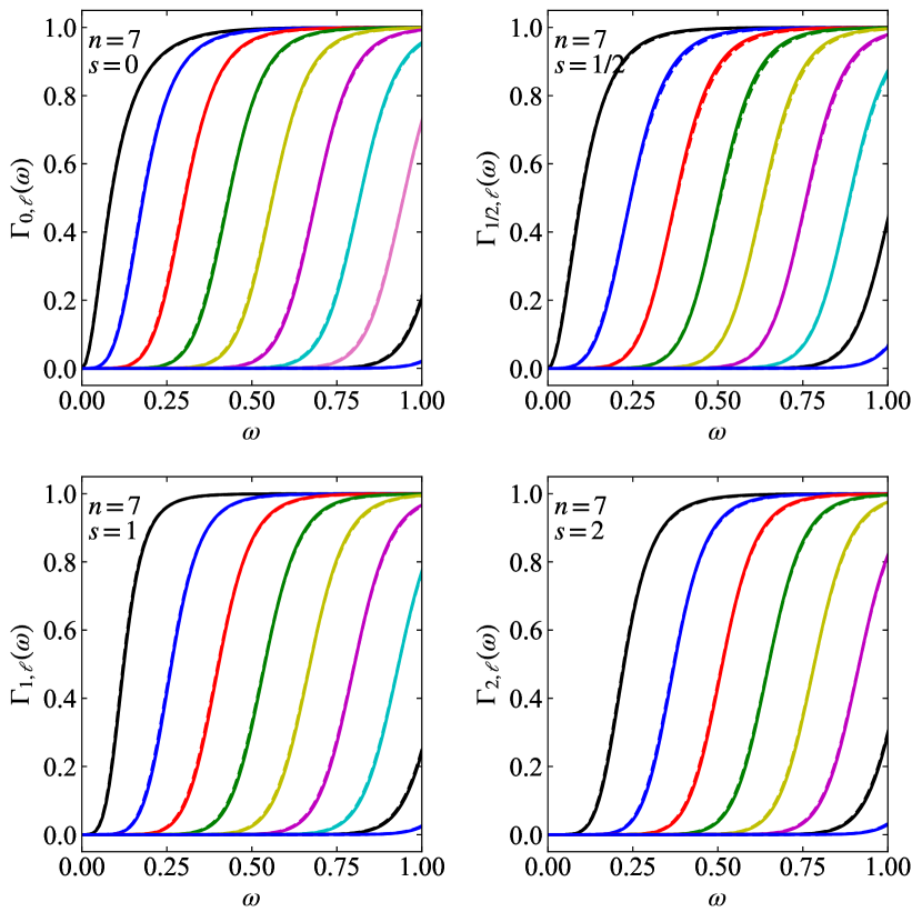
The fundamental calculated quantity is the transmission coefficient as a function of frequency for different black hole masses, number of extra dimensions, spin, and modes. Figure 4 shows transmission coefficients for and as a function of frequency for different modes. The solid lines are for NC black holes and dashed lines for ST black holes. The quantum number increases from going from left to right. A black hole mass of is used and corresponds to the NC black hole maximum temperature. We observe that the NC and ST black hole transmissions coefficients at this mass are very similar, differing slightly for higher . This is because they have a similar horizon radius at this mass of 5.68 for NC black holes and 5.76 for ST black holes.
If the horizon radius difference between NC and ST black holes is significantly different, the comparison changes. Figure 5 shows transmission coefficients for and as a function of frequency for different modes. A black hole mass of and are used for the NC black hole and ST black hole, respectively, corresponding to the NC black hole maximum temperature. In this case, significant differences are observed for a horizon radius of 5.68 for NC black holes and 6.48 for ST black holes.
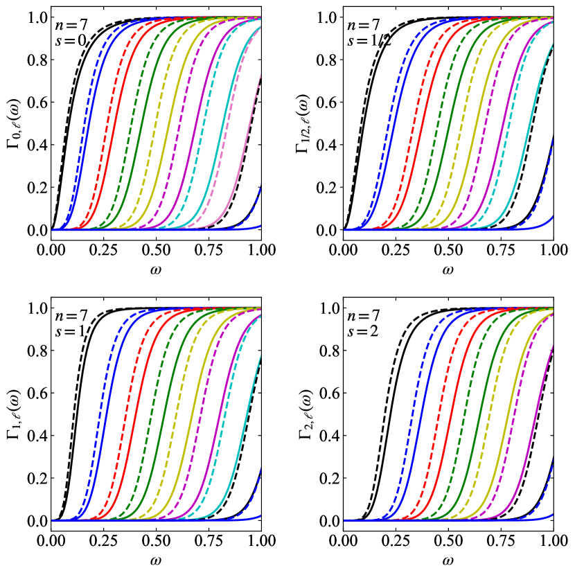
To examine more significant differences in transmission coefficients, a value for the black holes mass at the minimum NC black hole mass can be chosen and is shown in Figure 6. The horizon radius of the NC black hole is 2.32 and that of the ST black hole 4.02. We observe significant differences between NC and ST black hole transmission coefficients with increasing . The NC black hole transmission probabilities begin to rise at higher frequencies but rise more steeply than the ST transmission probabilities. This behaviour was first observed for spin 0 in Ref. [10].
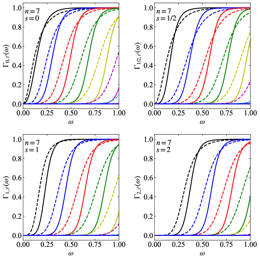
The number of effective modes used in the calculations can vary. The total number of modes considered are 15, 15, 14, 13 for , respectively. The number of effective modes giving a non-negligible contribution in the frequency range is different depending on , , and . Typically, and 1/2 have the same number of effective modes, while has one less and has two less modes. The and 2 cases have transmission coefficients that turn-on at higher frequencies relative to the and 1/2 cases, i.e. because of , the higher spins are missing the lower modes. As increases, the transmission coefficients become more spread out, and thus less modes will contribute to the given frequency range. The case has about four more modes than . The lowest masses we consider will have about three less effective modes than the highest masses we consider. The number of effective modes that will fit into the frequency range is largely determined by the spacing of the transmission coefficients in frequency.
Another important characteristic of the transmission coefficients is how steeply they rise with increasing frequency. In general, the turn-on steepness is largely independent of spin except for the and 1 modes. The more effective number of modes, the steeper the turn-on. Visually, the turn-on is most steep for and less step for .
The differences in transmission coefficients between NC and ST black holes depend significantly on their relative horizon radii. Typically a bigger horizon radius will give transmission coefficients that turn-on lower in frequency; the difference becoming more pronounced as increases. In addition, it is observed that at lower masses although the ST black hole transmission coefficients turn-on sooner, the NC black hole coefficients rise steeper and become higher before plateauing to unity, especially for .
5.2 Absorption cross sections
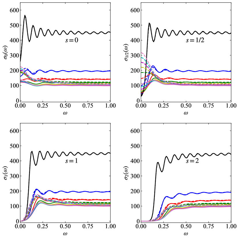
The absorption cross section depends on the weighted sum over of transmission coefficients and inversely as . Figure 7 shows cross sections versus frequency for . The solid lines are for NC black holes and dashed lines for ST black holes. Black hole masses corresponding to the NC black hole maximum temperature have been used; equal NC and ST black hole masses, in Table 1. Differences in cross sections are observed at low frequencies. These differences are most significant for and less pronounced for .
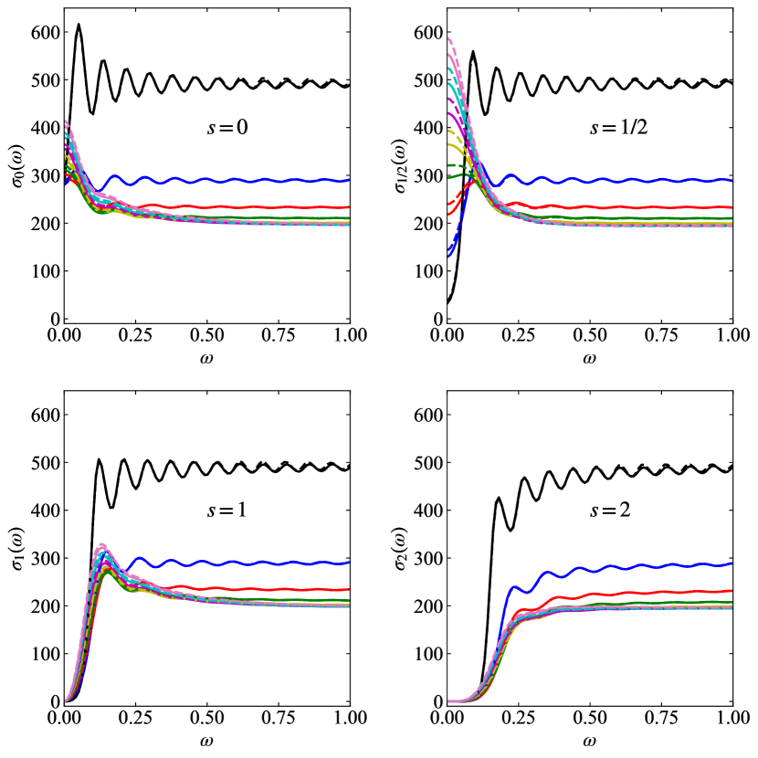
Hawking radiation for spin-2 fields in the ST metric was first discussed by Park [20]. Direct comparison is not possible since we use a different effective potential which is taken from Ref. [16] but originally comes from Ref. [21]. The difference in the general form of the potential appears significant but when substituting the particular ST metric, the difference is replacing the coefficient of the second term in Eq. (8d) by . Noteworthy in Ref. [20] is the acknowledgement that the spin-2 potential can become negative – potential well – for some masses (or radii), number of extra dimensions, and modes. The potential well can occur in the region . For the ST metric, the condition for non-negative potential is . If , the mode feel a potential well. The depth of the potential well, and height of the barrier, increase with increasing number of extra dimensions. A trade-off can occur between barrier suppression and well enhancement. For the ST case, this causes the –7 spin-2 cross sections to rise slightly faster at low-frequency than the –4 cross sections. The same observations are made for the NC case. However, the effect is small and will not concern use for the remainder of this paper.
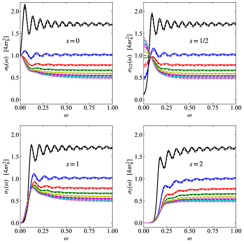
The differences in Figure 7 at low frequency are predominately due to differences in horizon area. It is enlightening to effectively remove these by scaling the cross sections by as shown in Figure 8. The cross sections are now in better agreement for but have almost constant residual differences for . These differences are due to the universal nature of the cross section – to be discussed later.
At the mass giving maximum NC black hole temperature, the horizon radius of the NC and ST black holes are similar. To examine larger differences due to the transmission coefficients, we take masses near the minimum NC back hole horizon; values from Table 10 (for numerical stability). Figure 9 shows significant differences for all but the low cases.
For ST black holes, the absorption cross section results are the same as Ref. [19]. Although the absorption cross section results for NC black holes and agree qualitatively with Ref. [10], they are quantitatively different 222We do not understand the normalization of Figure 7 in Ref. [10]. Figure 3 Ref. [10] shows values of at the maximum temperature. These values correspond to horizon areas of about which are in contradiction to what is shown in Figure 7 Ref. [10]..
The transmission coefficients for spin 0 and 1/2 turn on immediately for tiny frequencies, leading to finite absorption cross sections at zero frequency. Transmission coefficient for spin 1 and 2 are essential zero at , leading to an absorption cross section of zero at zero frequency. The usual oscillations are seen and the number of peaks correspond to the number of modes. The oscillation are more predominate at low where the transmission coefficients rise the steepest. After normalizing by the horizon radius, the absorption cross sections for NC black holes are higher than the ST back hole.
For spin 0, the low-frequency limit should correspond to the area of the black hole for both ST and NC black holes: . Numerically, for , we obtain the black hole area to better than 0.9% for both ST and NC black holes for high and low mass and for all number of dimensions and spins; except for for which it agrees to 1.7% for ST black holes of mass . For spin 1/2, the low-frequency limit is given by [22]
| (8t) |
which we are able to reproduce numerically to better than 0.4%, except for the case in which we obtain 2% agreement. We also mention that we obtain zero absorption cross section at for spin 1 and 2 fields from NC and ST black holes to 0.01%.
In the high-frequency limit, it has been shown that the absorption cross section approaches a universal geometrical optics limit of , where and is given by the solution to [23]. Using the ST metric, one obtains
| (8u) |
where is the ST horizon radius. This result was first obtained a long time ago [24]. In the case of the NC metric, we have calculated numerically. For , we obtain the optical cross section for ST and NC black holes to better than 3% for high mass, all number dimensions, and all spins. For low mass, the NC accuracy remains but the ST and case worsens by up to 5%. Visually, we already approach the geometrical limit for . Reproducing these known analytical values is a good test of the numerical validity of our calculations.
5.3 Particle spectra
The particle spectra have an additional dependence on temperature and the dependence on frequency is only indirectly through the sum of transmission coefficients and the statistical factor. This time it is not possible to take the minimum NC black hole mass (zero temperature) as the spectra will vanish due to the statistical factor. An interesting choice is to take the NC black hole mass at its maximum temperature. For the ST black hole comparison, logical choices are to take the same mass or the mass that gives the same temperature. If the same temperature is taken, the statistical factor in the particle spectra will be identical and the only difference will be the transmission coefficient sum part of the formula. First, we consider the case of equal mass which means the temperature of the ST black hole will be hotter, and hence lead to significantly more particle flux. Figure 10 shows particle spectra versus frequency for , and 2. The solid lines are for NC black holes and dashed lines for ST black holes. The number of extra dimensions increases from 0 to 7 as the curves move from bottom to top. Black hole masses corresponding to the NC black hole maximum temperature have been used, as shown in Table 1.
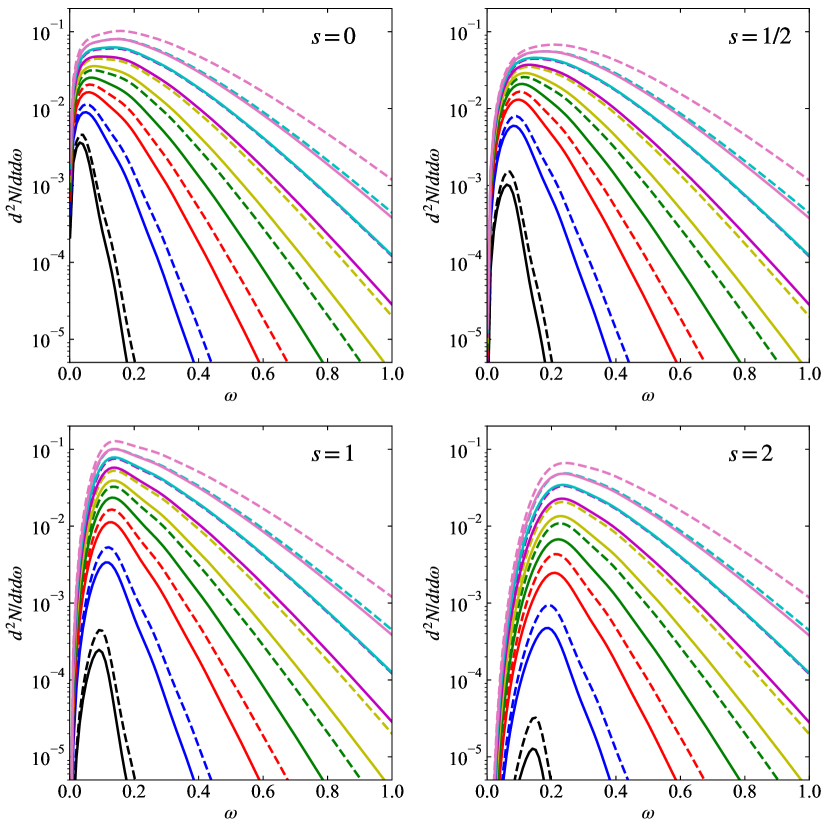
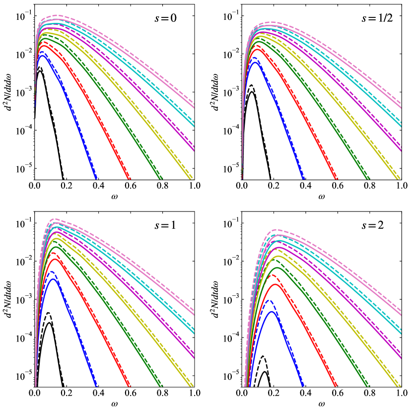
To remove the temperature dependence, different mass NC and ST black holes are compared. Figure 11 shows particle spectra versus frequency. Black hole masses for NC black holes and for ST black holes corresponding to the NC black hole maximum temperature have been used, as shown in Table 1.
5.4 Energy spectra
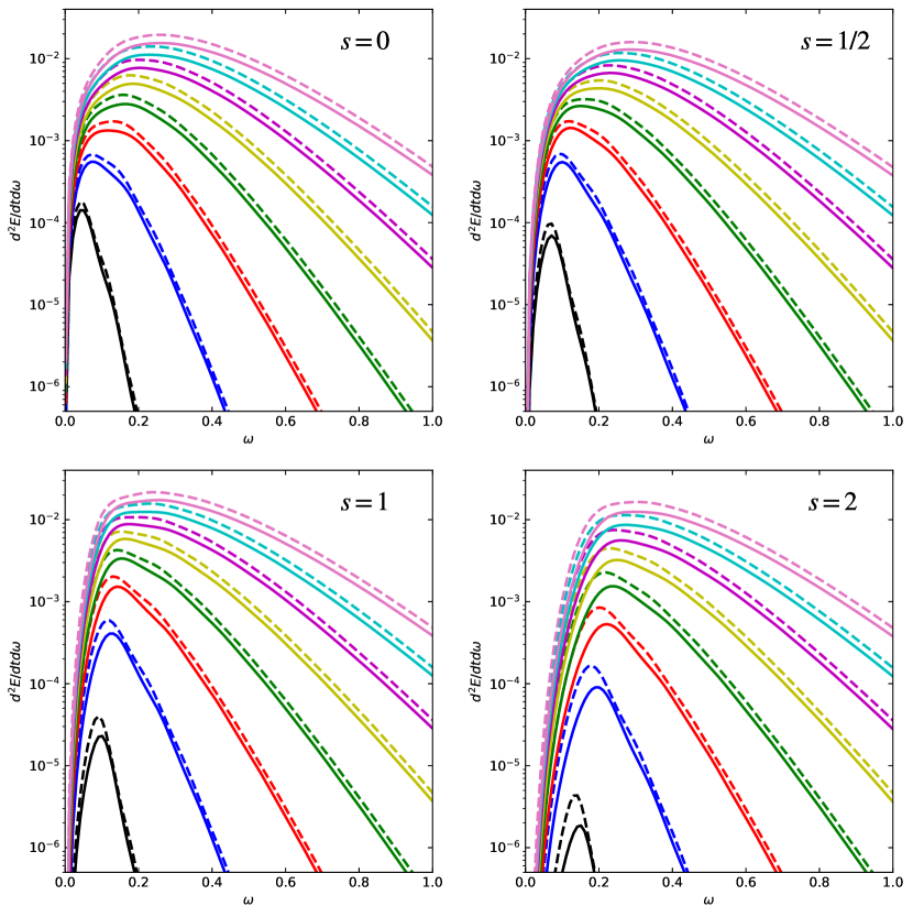
The energy spectra are similar to the particle spectra but include a multiplicative frequency factor. Figure 12 shows energy spectra versus frequency for and 2. The solid lines are for NC black holes and dashed lines for ST black holes. The number of extra dimensions increases from 0 to 7 as the curves move from bottom to top. Black hole masses corresponding to the NC black hole maximum temperature have been used, as shown in Table 1.
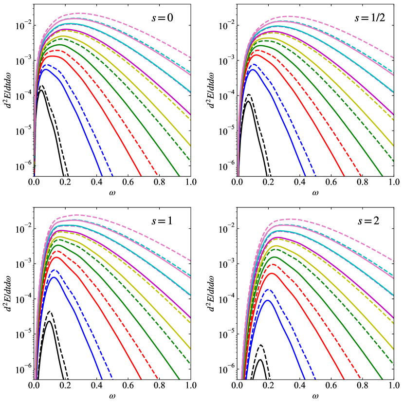
To remove the temperature dependence, different mass NC and ST black holes are compared. Figure 13 shows energy spectra versus frequency. Black hole masses for NC black holes and for ST black holes corresponding to the NC black hole maximum temperature have been used, as shown in Table 1.
5.5 Particle flux and total power
To make the comparison quantitative, we integrate the particle spectra and energy spectra over frequency out to to obtain the particle flux and power, respectively. Table 2 and Table 3 show the NC to ST particle flux ratios for the cases of equal mass and equal temperature, respectively. We observe the ratio of spin 0 and 1 fields are not very sensitive to number of extra dimensions for . The biggest change in particle flux ratio with number of dimensions is for spin 2.
-
0 1 2 3 4 5 6 7 0 0.73 0.71 0.70 0.70 0.70 0.70 0.70 0.71 1/2 0.65 0.69 0.70 0.71 0.71 0.72 0.72 0.72 1 0.54 0.60 0.63 0.65 0.67 0.68 0.69 0.69 2 0.40 0.49 0.53 0.57 0.59 0.61 0.63 0.64
-
0 1 2 3 4 5 6 7 0 0.80 0.79 0.79 0.79 0.79 0.79 0.79 0.79 1/2 0.71 0.77 0.79 0.80 0.80 0.81 0.81 0.81 1 0.59 0.67 0.71 0.74 0.75 0.76 0.77 0.78 2 0.44 0.54 0.60 0.64 0.67 0.69 0.71 0.72
Table 4 and Table 5 show the NC to ST power ratios for the cases of equal mass and equal temperature, respectively. The same observations can be made as for the particle fluxes.
-
0 1 2 3 4 5 6 7 0 0.67 0.64 0.62 0.62 0.62 0.62 0.63 0.63 1/2 0.61 0.63 0.63 0.63 0.63 0.63 0.64 0.64 1 0.51 0.57 0.59 0.60 0.61 0.62 0.63 0.63 2 0.39 0.46 0.50 0.53 0.55 0.57 0.59 0.60
-
0 1 2 3 4 5 6 7 0 0.82 0.80 0.79 0.79 0.79 0.79 0.79 0.80 1/2 0.74 0.79 0.80 0.80 0.80 0.80 0.81 0.81 1 0.63 0.71 0.75 0.77 0.78 0.79 0.79 0.80 2 0.47 0.58 0.64 0.68 0.70 0.72 0.74 0.75
Concentrating on NC geometry inspired black holes, we calculate the particle flux and total power for each number of extra dimensions and compare it to the case shown in Table 6 and Table 7, respectively. Direct comparison with Ref. [19] of the results for ST black holes (not shown) is not possible since the black hole mass used is not stated. The results are however, similar.
-
0 1 2 3 4 5 6 7 0 1 5 12 25 44 69 101 141 1/2 1 10 29 61 104 160 230 312 1 1 22 93 235 459 772 1179 1685 2 1 59 406 1354 3189 6149 10412 16131
-
0 1 2 3 4 5 6 7 0 1 9 32 84 174 316 519 794 1/2 1 15 60 153 311 551 887 1334 1 1 30 160 469 1031 1916 3187 4899 2 1 82 668 2512 6494 13504 24379 39872
Shown in Table 8 and Table 9 are the case of particle flux and power for each spin compared to the spin-0 case. Direct comparison with Ref. [19] of the results for ST black holes (not shown) is not possible since the black hole mass used is not stated. However, the results are the same as Ref. [19] for most cases, except for a difference of 1% for some spins.
-
0 1 0.33 0.08 0.005 1 1 0.68 0.38 0.06 2 1 0.78 0.62 0.15 3 1 0.79 0.77 0.25 4 1 0.78 0.87 0.33 5 1 0.76 0.93 0.41 6 1 0.74 0.97 0.47 7 1 0.73 0.99 0.53
-
0 1 0.50 0.17 0.01 1 1 0.86 0.61 0.14 2 1 0.92 0.86 0.30 3 1 0.91 0.97 0.44 4 1 0.89 1.03 0.55 5 1 0.87 1.05 0.63 6 1 0.85 1.06 0.69 7 1 0.84 1.07 0.74
6 Discussion
Transmission coefficients for spin 0, 1/2, 1, and 2 fields from NC geometry inspired black holes of extra dimension from 0 to 7 have been calculated. The NC black hole transmission coefficients are similar to the ST black hole transmission coefficients when their horizon radius are similar. However, there are major differences when the black hole masses are similar but the horizon radius are significantly different. The major difference in transmission coefficients is that the NC black hole transmission coefficients turn-on at slightly higher frequency. The differences between NC black hole and ST black hole transmission coefficients are about the same for all spins.
The absorption cross section of different spin fields from NC geometry inspired black holes of different number extra dimensions have been calculated. Significant differences in NC black hole and ST black hole absorption cross sections occur at low frequencies while the cross sections at high frequencies approach the geometrical optics limits. For masses near the minimum NC black hole mass, the differences are more apparent, particularly for higher dimensions.
The particle and energy spectra on the brane of different spin fields from NC geometry inspired black holes of different number of extra dimensions have been calculated. For equal masses, the NC black hole spectra are significantly lower than for ST black holes, mainly due to the lower temperature. However, at equal temperature the NC black hole spectra are still significantly lower than for ST black hole spectra.
When integrating the particle spectra over frequency the particle flux from NC black holes is significantly less than that from ST black holes. For spin-0 fields, the reduction can be from 0.70-0.80 depending on if the black holes have equal mass (lower number) or equal temperature (higher number). The dependence on the number of dimensions is small. For spin-1/2 fields, the ratio is from 0.65-0.81, also not too dependent on number of extra dimensions. For spin-1 fields, the ratio is 0.54-0.78. But for spin-2 fields, the reduction is most significant from 0.40-0.72, increasing with increasing number of dimensions. The general trends in the power are similar to the trends in the particle flux.
Considering the NC geometry inspired black hole emission on its own, it is common to compare the fluxes to the spin-0 case or the case. Increases in particle flux and power relative to the case are observed for increasing number of dimensions. The increase is most prominent for spin 2 and smallest for spin 0. The particle flux and power of spin-1/2 fields relative to spin-0 fields is less, with being the lowest and the highest for the particle flux and for power. The particle flux of spin-1 fields relative to spin-0 fields is less and decreases significantly with decreasing number of dimensions. The power of spin-1 fields relative to spin-0 fields is less or greater, depending on the number of dimensions; being significantly less for and slightly greater for . The spin-2 fields particle fluxes and power are always significantly less than for spin-0 fields, being 1% for .
We have presented greybody factors, absorption cross sections, and particle and energy spectra for all spin fields from higher-dimensional non-commutative geometry inspired black holes for the first time. The calculations are numerical and thus valid over the entire frequency range. The emission of higher spin fields, particularly graviton emission, could be useful for relating possible future observations of high-temperature black hole radiation to theory. The reduction in emission due to the greybody factors, not temperature, that we observe are hopefully model independent. This work represents another step towards possibly elucidating some aspects of quantum gravity.
Acknowledgments
We acknowledge the support of the Natural Sciences and Engineering Research Council of Canada (NSERC). Nous remercions le Conseil de recherches en sciences naturelles et en génie du Canada (CRSNG) de son soutien.
Appendix A Experimental constraints
The experimental lower bounds on and the maximum energy of the LHC will restrict the values of that can be probed by experiments at the LHC. We do not expect black holes to form for masses much less than . This give a lower bound on . We will consider only the hard limits on the Planck scale set by accelerator experiments [25, 26]: TeV for , TeV for , TeV for , TeV for , TeV for , and TeV for . The maximum mass of the black hole is likely to be limited by the statistics of the maximum parton energies in a proton-proton interaction but in no case can it be larger than the proton-proton center-of-mass energy. Thus, we will only be interested in the case where the minimum black hole mass is below the LHC current maximum energy of 13.6 TeV and above the experimental lower bound on the Planck scale.
-
0 3.02 47.9 1 2.68 63.2 2 2.51 65.2 0.248 0.265 3 2.41 58.8 0.361 0.406 4 2.34 48.6 0.460 0.524 5 2.29 37.9 0.546 0.619 6 2.26 28.2 0.621 0.699 7 2.23 20.3 0.686 0.978
We obtain a valid range of for each number of extra dimensions by restricting the minimum black hole mass at the LHC to be in the range TeV/, as discussed above. The results are given in Table 10. We see that is very restricted and there is no single value of that lies in the allowed range for all number of extra dimensions.
To study the phenomenology of NC inspired black holes at the LHC experiments one can take above the experimental limits and the following values for , for , for , for , for , and for .
References
References
- [1] Piero Nicolini, Anais Smailagic, and Euro Spallucci. Noncommutative geometry inspired Schwarzschild black hole. Phys. Lett. B, 632:547–551, 2006.
- [2] Stefano Ansoldi, Piero Nicolini, Anais Smailagic, and Euro Spallucci. Noncommutative geometry inspired charged black holes. Phys. Lett. B, 645:261–266, 2007.
- [3] Thomas G. Rizzo. Noncommutative inspired black holes in extra dimensions. JHEP, 09(021), 2006.
- [4] Euro Spallucci, Anais Smailagic, and Piero Nicolini. Non-commutative geometry inspired higher-dimensional charged black holes. Phys. Lett. B, 670:449–454, 2009.
- [5] Piero Nicolini. Noncommutative black holes, the final appeal to quantum gravity: A review. Int. J. Mod. Phys. A, 24:1229–1308, 2009.
- [6] Rabin Banerjee, Bibhas Ranjan Majhi, and Saurav Samanta. Noncommutative Black Hole Thermodynamics. Phys. Rev. D, 77:124035, 2008.
- [7] Kourosh Nozari and S. Hamid Mehdipour. Hawking Radiation as Quantum Tunneling from Noncommutative Schwarzschild Black Hole. Class. Quant. Grav., 25:175015, 2008.
- [8] Rabin Banerjee, Sunandan Gangopadhyay, and Sujoy Kumar Modak. Voros product, Noncommutative Schwarzschild Black Hole and Corrected Area Law. Phys. Lett. B, 686:181–187, 2010.
- [9] Douglas M. Gingrich. Noncommutative geometry inspired black holes in higher dimensions at the LHC. JHEP, 05(022), 2010.
- [10] Piero Nicolini and Elizabeth Winstanley. Hawking emission from quantum gravity black holes. JHEP, 11(075), 2011.
- [11] R. L. Workman and Others. Review of Particle Physics. PTEP, 2022:083C01, 2022.
- [12] Saul A. Teukolsky. Perturbations of a rotating black hole. 1. Fundamental equations for gravitational electromagnetic and neutrino field perturbations. Astrophys. J., 185:635–647, 1973.
- [13] William H. Press and Saul A. Teukolsky. Perturbations of a rotating black hole. II. Dynamical stability of the Kerr metric. Astrophys. J., 185:649–674, October 1973.
- [14] S. A. Teukolsky and W. H. Press. Perturbations of a rotating black hole. III - Interaction of the hole with gravitational and electromagnetic radiation. Astrophys. J., 193:443–461, 1974.
- [15] S. Chandrasekhar. The mathematical theory of black holes. Oxford University Press, 1983.
- [16] Alexandre Arbey, Jérémy Auffinger, Marc Geiller, Etera R. Livine, and Francesco Sartini. Hawking radiation by spherically-symmetric static black holes for all spins: Teukolsky equations and potentials. Phys. Rev. D, 103(10):104010, 2021.
- [17] Alexandre Arbey, Jérémy Auffinger, Marc Geiller, Etera R. Livine, and Francesco Sartini. Hawking radiation by spherically-symmetric static black holes for all spins. II. Numerical emission rates, analytical limits, and new constraints. Phys. Rev. D, 104(8):084016, 2021.
- [18] Finnian Gray and Matt Visser. Greybody factors for Schwarzschild black holes: Path-ordered exponentials and product integrals. Universe, 4(9):93, 2018.
- [19] Chris M. Harris and Panagiota Kanti. Hawking radiation from a (4+n)-dimensional black hole: Exact results for the Schwarzschild phase. JHEP, 10(014), 2003.
- [20] D. K. Park. Hawking radiation of the brane-localized graviton from a (4+n)-dimensional black hole. Class. Quant. Grav., 23:4101–4110, 2006.
- [21] Flora Moulin, Aurélien Barrau, and Killian Martineau. An overview of quasinormal modes in modified and extended gravity. Universe, 5(9):202, 2019.
- [22] Panagiota Kanti and John March-Russell. Calculable corrections to brane black hole decay. 2. Greybody factors for spin 1/2 and 1. Phys. Rev. D, 67:104019, 2003.
- [23] Yves Decanini, Gilles Esposito-Farese, and Antoine Folacci. Universality of high-energy absorption cross sections for black holes. Phys. Rev. D, 83:044032, 2011.
- [24] Roberto Emparan, Gary T. Horowitz, and Robert C. Myers. Black holes radiate mainly on the brane. Phys. Rev. Lett., 85:499–502, 2000.
- [25] V. M. Abazov et al. Search for large extra dimensions via single photon plus missing energy final states at = 1.96-TeV. Phys. Rev. Lett., 101:011601, 2008.
- [26] Georges Aad et al. Search for new phenomena in events with an energetic jet and missing transverse momentum in collisions at =13 TeV with the ATLAS detector. Phys. Rev. D, 103(11):112006, 2021.