Greedy Recombination Interpolation Method (GRIM)
Abstract
In this paper we develop the Greedy Recombination Interpolation Method (GRIM) for finding sparse approximations of functions initially given as linear combinations of some (large) number of simpler functions. In a similar spirit to the CoSaMP algorithm, GRIM combines dynamic growth-based interpolation techniques and thinning-based reduction techniques. The dynamic growth-based aspect is a modification of the greedy growth utilised in the Generalised Empirical Interpolation Method (GEIM). A consequence of the modification is that our growth is not restricted to being one-per-step as it is in GEIM. The thinning-based aspect is carried out by recombination, which is the crucial component of the recent ground-breaking convex kernel quadrature method. GRIM provides the first use of recombination outside the setting of reducing the support of a measure. The sparsity of the approximation found by GRIM is controlled by the geometric concentration of the data in a sense that is related to a particular packing number of the data. We apply GRIM to a kernel quadrature task for the radial basis function kernel, and verify that its performance matches that of other contemporary kernel quadrature techniques.
1 Introduction
This article considers finding sparse approximations of functions with the aim of reducing computational complexity. Applications of sparse representations are wide ranging and include the theory of compressed sensing [DE03, CT05, Don06, CRT06], image processing [EMS08, BMPSZ08, BMPSZ09], facial recognition [GMSWY09], data assimilation [MM13], explainability [FMMT14, DF15], sensor placement in nuclear reactors [ABGMM16, ABCGMM18], reinforcement learning [BS18, HS19], DNA denoising [KK20], and inference acceleration within machine learning [ABDHP21, NPS22].
Loosely speaking, the commonly shared aim of sparse approximation problems is to approximate a complex system using only a few elementary features. In this generality, the problem is commonly tackled via Least Absolute Shrinkage and Selection Operator (LASSO) regression, which involves solving a minimisation problem under -norm constraints. Constraining the -norm is a convex relaxation of constraining the -pseudo-norm, which counts the number of non-zero components of a vector. Since is the smallest positive real number for which the -norm is convex, constraining the -norm can be viewed as the best convex approximation of constraining the -pseudo-norm (i.e. constraring the number of non-zero components). Implementations of LASSO techniques can lead to near optimally sparse solutions in certain contexts [DET06, Tro06, Ela10]. The terminology ”LASSO” originates in [Tib96], though imposing -norm constraints is considered in the earlier works [CM73, SS86]. More recent LASSO-type techniques may be found in, for example, [LY07, DGOY08, GO09, XZ16, TW19].
Alternatives to LASSO include the Matching Pursuit (MP) sparse approximation algorithm introduced in [MZ93] and the CoSaMP algorithm introduced in [NT09]. The MP algorithm greedily grows a collection of non-zero weights one-by-one that are used to construct the approximation. The CoSaMP algorithm operates in a similar greedy manner but with the addition of two key properties. The first is that the non-zero weights are no longer found one-by-one; groups of several non-zero weights may be added at each step. Secondly, CoSaMP incorporates a naive prunning procedure at each step. After adding in the new weights at a step, the collection is then pruned down by retaining only the -largest weights for a chosen integer . The ethos of CoSaMP is particularly notworthy for our purposes.
In this paper we assume that the system of interest is known to be a linear combination of some (large) number of features. Within this setting the goal is to identify a linear combination of a strict sub-collection of the features (i.e. not all the features) that gives, in some sense, a good approximation of the system (i.e. of the original given linear combination of all the features). Depending on the particular context considered, techniques for finding such sparse approximations include the pioneering Empirical Interpolation Method [BMNP04, GMNP07, MNPP09], its subsequent generalisation the Generalised Empirical Interpolation Method (GEIM) [MM13, MMT14], Pruning [Ree93, AK13, CHXZ20, GLSWZ21], Kernel Herding [Wel09a, Wel09b, CSW10, BLL15, BCGMO18, TT21, PTT22], Convex Kernel Quadrature [HLO21], and Kernel Thinning [DM21a, DM21b, DMS21]. The LASSO approach based on -regularisation can still be used within this framework.
It is convenient for our purposes to consider the following loose categorisation of techniques for finding sparse approximations in this setting; those that are growth-based, and those that are thinning-based. Growth-based methods seek to inductively increase the size of a sub-collection of features, until the sub-collection is rich enough to well-approximate the entire collection of features. Thinning-based methods seek to inductively identify features that may be discarded without significantly affecting how well the remaining features can approximate the original entire collection. Of the techniques mentioned above, MP, EIM, GEIM and Kernel Herding are growth-based, whilst LASSO, Convex Kernel Quadrature and Kernel Thinning are thinning-based. An important observation is that the CoSaMP algorithm combines both growth-based and thinning-based techniques.
In this paper we work in the setting considered by Maday et al. when introducing GEIM [MM13, MMT14, MMPY15]. Namely, we let be a real Banach space and be a (large) positive integer. Assume that is a collection of non-zero elements, and that . Consider the element defined by . Let denote the dual of and suppose that is a finite subset with cardinality . We use the terminology that the set consists of the features whilst the set consists of data. Then we consider the following sparse approximation problem. Given , find an element such that the cardinality of the set is less than and that is close to throughout in the sense that, for every , we have .
The tasks of approximating sums of continuous functions on finite subsets of Euclidean space, cubature for empirical measures, and kernel quadrature for kernels defined on finite sets are included as particular examples within this general mathematical framework (see Section 2) for full details). The inclusion of approximating a linear combination of continuous functions within this general framework ensures that several machine learning related tasks are included. For example, each layer of a neural network is typically given by a linear combination of continuous functions. Hence the task of approximating a layer within a neural network by a sparse layer is covered within this general framework. Observe that there is no requirement that the original layer is fully connected; in particular, it may itself already be a sparse layer. Consequently, any approach to the approximation problem covered in the general framework above could be used to carry out the reduction step (in which a fixed proportion of a models weights are reduced to zero) in the recently proposed sparse training algorithms [GLMNS18, EJOPR20, LMPY21, JLPST21, FHLLMMPSWY23].
The GEIM approach developed by Maday et al. [MM13, MMT14, MMPY15] involves dynamically growing a subset of the features and a subset of the date. At each step a new feature from is added to , and a new piece of data from is added to . An approximation of is then constructed via the following interpolation problem. Find a linear combination of the elements in that coincides with throughout the subset . This dynamic growth is feature-driven in the following sense. The new feature to be added to is determined, and this new feature is subsequently used to determine how to extend the collection of linear functionals on which an approximation will be required to match the target.
The growth is greedy in the sense that the element chosen to be added to is, in some sense, the one worst approximated by the current collection . If we let be the newly selected feature and be the linear combination of the previously selected features in that coincides with on , then the element to be added to is the one achieving the maximum absolute value when acting on . A more detailed overview of GEIM can be found in Section 2 of this paper; full details of GEIM may be found in [MM13, MMT14, MMPY15].
Momentarily restricting to the particular task of kernel quadrature, the recent thinning-based Convex Kernel Quadrature approach proposed by Satoshi Hayakawa, the first author, and Harald Oberhauser in [HLO21] achieves out performs existing techniques such as Monte Carlo, Kernel Herding [Wel09a, Wel09b, CSW10, BLL15, BCGMO18, PTT22], Kernel Thinning [DM21a, DM21b, DMS21] to obtain new state-of-the-art results. Central to this approach is the recombination algorithm [LL12, Tch15, ACO20]. Originating in [LL12] as a technique for reducing the support of a probability measure whilst preserving a specified list of moments, at its core recombination is a method of reducing the number of non-zero components in a solution of a system of linear equations whilst preserving convexity.
An improved implementation of recombination is given in [Tch15] that is significantly more efficient than the original implementation in [LL12]. A novel implementation of the method from [Tch15] was provided in [ACO20]. A modified variant of the implementation from [ACO20] is used in the convex kernel quadrature approach developed in [HLO21]. A method with the same complexity as the original implementation in [LL12] was introduced in the works [FJM19, FJM22].
Returning to our general framework, we develop the Greedy Recombination Interpolation Method (GRIM) which is a novel hybrid combination of the dynamic growth of a greedy selection algorithm, in a similar spirit to GEIM [MM13, MMT14, MMPY15], with the thinning reduction of recombination that underpins the successful convex kernel quadrature approach of [HLO21]. GRIM dynamically grows a collection of linear functionals . After each extension of , we apply recombination to find an approximation of that coincides with throughout (cf. the recombination thinning Lemma 3.1). Subsequently, for a chosen integer , we extend by adding the linear functionals from achieving the largest absolute values when applied to the difference between and the current approximation of (cf. Section 4). We inductively repeat these steps a set number of times. Evidently GRIM is a hybrid of growth-based and thinning-based techniques in a similar spirit to the CoSaMP algorithm [NT09].
Whilst the dynamic growth of GRIM is in a similar spirit to that of GEIM, there are several important distinctions between GRIM and GEIM. The growth in GRIM is data-driven rather than feature-driven. The extension of the data to be interpolated with respect to in GRIM does not involve making any choices of features from . The new information to be matched is determined by examining where in the current approximation is furthest from the target (cf. Section 4).
Expanding on this point, we only dynamically grow a subset of the data and do not grow a subset of the features. In particular, we do not pre-determine the features that an approximation will be a linear combination of. Instead, the features to be used are determined by recombination (cf. the recombination thinning Lemma 3.1). Indeed, besides an upper bound on the number of features being used to construct an approximation (cf. Section 4), we have no control over the features used. Allowing recombination and the data to determine which features are used means there is no requirement to use the features from one step at subsequent steps. There is no requirement that any of the features used at one specific step must be used in any of the subsequent steps.
GRIM is not limited to extending the subset by a single linear functional at each step. GRIM is capable of extending by linear functionals for any given integer (modulo restrictions to avoid adding more linear functionals than there are in the original subset itself). The number of new linear functionals to be added at a step is a hyperparameter that can be optimised during numerical implementations.
Unlike [HLO21], our use of recombination is not restricted to the setting of reducing the support of a discrete measure. After each extension of , we use recombination [LL12, Tch15, ACO20] to find an element satisfying that throughout . Recombination is applied to the linear system determined by the combination of the set , for a given we get the equation , and the sum of the coefficients (i.e. the trivial equation ) (cf. the recombination thinning Lemma 3.1).
Our use of recombination means, in particular, that GRIM can be used for cubature and kernel quadrature (cf. Sections 2 and 4). Since recombination preserves convexity [LL12], the benefits of convex weights enjoyed by the convex kernel quadrature approach in [HLO21] are inherited by GRIM (cf. Section 2).
Moreover, at each step we optimise our use of recombination over multiple permutations of the orderings of the equations determining the linear system to which recombination is applied (cf. the Banach Recombination Step in Section 4). The number of permutations to be considered at each step gives a parameter that may be optimised during applications of GRIM.
Whilst we analyse the complexity cost of the Banach GRIM algorithm (cf. Section 5), computational efficiency is not our top priorities. GRIM is designed to be a one-time tool; it is applied a single time to try and find a sparse approximation of the target system . The cost of its implementation is then recouped through the repeated use of the resulting approximation for inference via new inputs. Thus GRIM is ideally suited for use in cases where the model will be repeatedly computed on new inputs for the purpose of inference/prediction. Examples of such models include, in particular, those trained for character recognition, medical diagnosis, and action recognition.
With this in mind, the primary aim of our complexity cost considerations is to verify that implementing GRIM is feasible. We verify this by proving that, at worst, the complexity cost of GRIM is where is the number of features in , is the number of linear functionals forming the data , and is the maximum number of shuffles considered during each application of recombination (cf. Lemma 5.3).
The remainder of the paper is structured as follows. In Section 2 we fix the mathematical framework that will be used throughout the article and motivate its consideration. In particular, we illustrate some specific examples covered by our framework. Additionally, we summarise the GEIM approach of Maday et al. [MM13, MMT14, MMPY15] and highlight the fundamental differences in the philosophies underlying GEIM and GRIM.
An explanation of the recombination algorithm and its use within our setting is provided in subsection 3. In particular, we prove the Recombination Thinning Lemma 3.1 detailing our use of recombination to find coinciding with on a given finite subset .
The Banach GRIM algorithm is both presented and discussed in Section 4. We formulate the Banach Extension Step governing how we extend an existing collection of linear functionals , the Banach Recombination Step specifying how we use the recombination thinning Lemma 3.1 in the Banach GRIM algorithm, and provide an upper bounds for the number of features used to construct the approximation at each step.
The complexity cost of the Banach GRIM algorithm is considered in Section 5. We prove Lemma 5.3 establishing the complexity cost of any implementation of the Banach GRIM algorithm, and subsequently establish an upper bound complexity cost for the most expensive implementation.
The theoretical performance of the Banach GRIM algorithm is considered in Section 6. Theoretical guarantees in terms of a specific geometric property of are established for the Banach GRIM algorithm in which a single new linear functional is chosen at each step (cf. the Banach GRIM Convergence Theorem 6.2). The specific geometric property is related to a particular packing number of in (cf. Subsection 6.2). The packing number of a subset of a Banach space is closely related to the covering number of the subset. Covering and packing numbers, first studied by Kolmogorov [Kol56], arise in a variety of contexts including eigenvalue estimation [Car81, CS90, ET96], Gaussian Processes [LL99, LP04], and machine learning [EPP00, SSW01, Zho02, Ste03, SS07, Kuh11, MRT12, FS21]
In Section 7 we compare the performance of GRIM against other reduction techniques on three tasks. The first is an -approximation task motivated by an example in [MMPY15]. The second is a kernel quadrature task using machine learning datasets as considered in [HLO21]. In particular, we illustrate that GRIM matches the performance of the tailor-made convex kernel quadrature technique developed in [HLO21]. The third task is approximating the action recognition model from [JLNSY17] for the purpose of inference acceleration. In particular, this task involves approximating a function in a pointwise sense that is outside the Hilbert space framework of the proceeding two examples. Acknowledgements: This work was supported by the DataSıg Program under the EPSRC grant ES/S026347/1, the Alan Turing Institute under the EPSRC grant EP/N510129/1, the Data Centric Engineering Programme (under Lloyd’s Register Foundation grant G0095), the Defence and Security Programme (funded by the UK Government) and the Hong Kong Innovation and Technology Commission (InnoHK Project CIMDA). This work was funded by the Defence and Security Programme (funded by the UK Government).
2 Mathematical Framework & Motivation
In this section we rigorously formulate the sparse approximation problem that GRIM will be designed to tackle. Further, we briefly summarise the Generalised Empirical Interpolation Method (GEIM) of Maday et al. [MM13, MMT14, MMPY15] to both highlight some of the ideas we utilise in GRIM, and to additionally highlight the key novel properties not satisfied by GEIM that will be satisfied by GRIM. We first fix the mathematical framework in which we will work for the remainder of this paper.
Let be a Banach space and be a (large) positive integer. Assume that is a collection of non-zero elements, and that . Consider the element defined by
| (2.1) |
Let denote the dual of and suppose that is a finite subset of cardinality . We use the terminology that the set consists of features whilst the set consists of data. We consider the following sparse approximation problem. Given , find an element such that the cardinality of the set is less than and that is close to throughout in the sense that, for every , we have .
The task of finding a sparse approximation of a sum of continuous functions, defined on a finite set of Euclidean space, is within this framework. More precisely, let , , be a finite subset, and, for each , be a continuous function . Then finding a sparse approximation of the continuous function is within this framework. To see this, first let be the standard basis of that is orthonormal with respect to the Euclidean dot product on . Then note that for each point and every the mapping determines a linear functional that is in the dual space . Denote this linear functional by . Therefore by choosing , , and , we see that this problem is within our framework. Here we are also using the observation that if satisfy, for every and every , that , then we have for a constant depending on the particular norm chosen on . Thus finding an approximation of that satisfies, for every , that allows us to conclude that .
The cubature problem [Str71] for empirical measures, which may be combined with sampling to offer an approach to the cubature problem for general signed measures, is within this framework. More precisely, let , , , and denote the collection of finite signed measures on . Recall that can be viewed as a subset of by defining, for and , . Consider the empirical measure and, for , define by . Then the choices that , , and, for a given , illustrate that the cubature problem of reducing the support of whilst preserving its moments of order no greater than is within our framework.
Moreover the Kernel Quadrature problem for empirical probability measures is within our framework. To be more precise, let be a finite set and is a Reproducing Kernel Hilbert Space (RKHS) associated to a positive semi-definite symmetric kernel function (appropriate definitions can be found, for example, in [BT11]). In this case where, for , the function is defined by (see, for example, [BT11]).
In this context one can consider the Kernel Quadrature problem, for which the Kernel Herding [Wel09a, Wel09b, CSW10, BLL15, BCGMO18, TT21, PTT22], Convex Kernel Quadrature [HLO21] and Kernel Thinning [DM21a, DM21b, DMS21] methods have been developed. Given a probability measure the Kernel Quadrature problem involves finding, for some , points and weights and such that the measure approximates in the sense that, for every , we have . Additionally requiring the weights to be convex in the sense that they are all positive and sum to one (i.e. and ) ensures both better robustness properties for the approximation and better estimates when the -fold product of quadrature formulas is used to approximate on ; see [HLO21].
A consequence of is that linearity ensures that this approximate equality will be valid for all provided it is true for every . The inclusion means that the subset can be viewed as a finite subset of the dual space . The choice of and illustrates that the Kernel Quadrature problem for empirical probability distributions is within the framework we consider.
The framework we consider is the same as the setup for which GEIM was developed by Maday et al. [MM13, MMT14, MMPY15]. It is useful to briefly recall this method. GEIM
-
(A)
-
•
Find and .
-
•
Define , , , and an operator by setting for every .
-
•
Observe that, given any , we have .
-
•
-
(B)
Proceed recursively via the follwing inductive step for .
-
•
Suppose we have found subsets and , and an operator satisfying, for every , that for every .
-
•
Find and .
-
•
Define
and .
-
•
Construct operator by defining
for . Direct computation verifies that, whenever and , we have .
-
•
The algorithm provides a sequence , of approximations of . However, GEIM is intended to control the -norm of the difference between and its approximation, i.e. to have be small for a suitable integer . This aim requires additional assumptions to be made regarding the data which we do not impose (see [MMT14] for details). Recall that we aim only to approximate over the data , i.e. we seek an approximation such that is small for every . A consequence of this difference is that certain aspects of GEIM are not necessarily ideal for our task.
Firstly, the growth of the subset to is feature-driven. That is, a new feature from to be used by the next approximation is selected, and then this new feature is used to determine the new functional from to be added to the collection on which we require the approximation to coincide with the target (cf. GEIM (B)). Since we only seek to approximate over the data , data-driven growth would be preferable. That is, we would rather select the new information from to be matched by the next approximation before any consideration is given to determining which features from will be used to construct the new approximation.
Secondly, related to the first aspect, the features from to be used to construct are predetermined. Further, the features used to construct are forced to be included in the features used to construct for any . This restriction is not guaranteed to be sensible; it is conceivable that the features that work well at one stage are disjoint from the features that work well at another. We would prefer that the features used to construct an approximation be determined by the target and the data selected from on which we require the approximation to match . This would avoid retaining features used at one step that become less effective at later steps, and could offer insight regarding which of the features in are sufficient to capture the behaviour of on .
Thirdly, at each step GEIM can provide an approximation for any . That is, for , the element is a linear combination of the elements in that coincides with on . Requiring the operator to provide such an approximation for every stops the method from exploiting any advantages available for the particular choice of . As we only aim to approximate itself, we would prefer to remove this requirement and allow the method the opportunity to exploit advantages resulting from the specific choice of .
All three aspects are addressed in GRIM. The greedy growth of a subset , determining the functionals in at which an approximation is required to agree with is data-driven. At each step the desired approximation is found using recombination [LL12, Tch15] so that the features used to construct the approximation are determined by and the subset and, in particular, are not predetermined. This use of recombination ensures both that GRIM only produces approximations of , and that GRIM can exploit advantages resulting from the specific choice of .
3 Recombination Thinning
In this section we illustrate how, given a finite collection of linear functionals, recombination [LL12, Tch15] can be used to find an element that coincides with throughout , provided we can compute the values for every and every linear functional . The recombination algorithm was initially introduced by Christian Litterer and the first author in [LL12]; a substantially improved implementation was provided in the PhD thesis of Maria Tchernychova [Tch15]. A novel implementation of the method from [Tch15] was provided in [ACO20]. A method with the same complexity as the original implementation in [LL12] was introduced in the works [FJM19, FJM22]. Recombination has been applied in a number of contexts including particle filtering [LL16], kernel quadrature [HLO21], and mathematical finance [NS21].
For the readers convenience we briefly overview the ideas involved in the recombination algorithm. For this illustrative purpose consider a linear system of equations where , , , and with . We assume, for every , that . Recombination relies on the simple observation that this linear system is preserved under translations of by elements in the kernel of the matrix . To be more precise, if satisfies that , and if and , then also satisfies that . The recombination algorithm makes use of linearly independent elements in the to reduce the number of non-zero entries in the solution vector .
As outlined in [LL12], this could in principle be done as follows. First, we choose a basis for the kernel of . Computing the Singular Value Decomposition (SVD) of gives a method of finding such a basis that is well-suited to dealing with numerical instabilities. Supposing that , let be a basis of found via SVD. For each denote the coefficients of by .
Consider the element . Choose such that
| (3.1) |
Replace by the vector . The new remains a solution to , and now additionally satisfies that . Moreover, for every such that , our choice of in (3.1) ensures that . Finally, for , replace by to ensure that . This final alteration allows us to repeat the process for the new using the new in place of since the addition of any scalar multiple of to will not change the fact that .
After iteratively repeating this procedure for , we obtain a vector whose coefficients are all non-negative, with at most of the coefficients being non-zero, and still satisfying that . That is, the original solution has been reduced to a new solution with at least fewer non-zero coefficients than the original solution .
Observe that the positivity of the original coefficients is weakly preserved. That is, if we let denote the coefficients of the vector , then for each we have that . One consequence of this preservation is that recombination can be used to reduce the support of an empirical measure whilst preserving a given finite collection of moments [LL12]. Moreover, this property is essential to the ground-breaking state-of-the-art convex kernel quadrature method developed by Satoshi Hayakawa, the first author, and Harald Oberhauser in [HLO21].
The implementation of recombination proposed in [LL12] iteratively makes use of the method outlined above, for , applied to linear systems arising via sub-dividing the original system. The improved tree-based method developed by Maria Tchernychova in [Tch15] provides a significantly more efficient implementation. A geometrically greedy algorithm is proposed in [ACO20] to implement the algorithm of [Tch15]. In the setting of our example above, it follows from [Tch15] that the complexity of the recombination algorithm is .
Having outlined the recombination method, we turn our attention to establishing the following result regarding the use of recombination in our setting.
Lemma 3.1 (Recombination Thinning).
Assume is a Banach space with dual space , that , and that . Define . Let be a collection of non-zero elements and . Suppose and consider the element defined by . Then recombination can be applied to find non-negative coefficients and indices satisfying that
| (3.2) |
and such that the element defined by
| (3.3) |
Finally, the complexity of this use of recombination is .
Proof of Lemma 3.1.
Assume is a Banach space with dual space , that , and that . Define . Let be a collection of non-zero elements and . Suppose and Consider the element defined by .
The values and the sum of the coefficients give rise to the linear system of equations
| (3.4) |
which we denote more succinctly by .
Since the coefficients are positive, we are able to apply recombination [LL12, Tch15] to this linear system. Combined with the observation that , an application of recombination returns an element satisfying the following properties. Firstly, for each the coefficient is non-negative. Secondly, there are at most indices for which .
Let . Take to be the indices for which . Then, for each , we set . Define an element by (cf. (3.3)). Recall that recombination ensures that is a solution to the linear system (3.4). Hence the equation corresponding to the top row of the matrix tells us that
| (3.5) |
Moreover, given any , the equation corresponding to row of the matrix tells us that
| (3.6) |
If then (3.5) and (3.6) are precisely the equalities claimed in (3.2) and (3.3). If then . Set and choose any indices . Evidently we have that and, for each , that . Consequently, (3.5) and (3.6) are once again precisely the equalities claimed in (3.2) and (3.3).
4 The Banach GRIM Algorithm
In this section we detail the Banach GRIM algorithm. The following Banach Extension Step is used to grow a collection of linear functionals from at which we require our next approximation of to agree with . Banach Extension Step
Assume . Let . Let such that . Take
| (4.1) |
Inductively for take
| (4.2) |
Once have been defined, we extend to . For each choice of subset , we use recombination (cf. Lemma 3.1) to find agreeing with throughout . Theoretically, Lemma 3.1 verifies that recombination can be used to find an approximation of for which for all linear functionals for a given subset . However, implementations of recombination inevitably result in numerical errors. That is, the returned coefficients will only solve the equations modulo some (ideally) small error term. To account for this in our analysis, whenever we apply Lemma 3.1 we will only assume that the resulting approximation is close to at each functional . That is, for each , we have that for some (small) constant .
Recall (cf. Section 3) that if recombination is applied to a linear system corresponding to a matrix , then a Singular Value Decomposition SVD of the matrix is used to find a basis for . Re-ordering the rows of the matrix (i.e. changing the order in which the equations are considered) can potentially result in a different basis for being selected. Thus shuffling the order of the equations can affect the approximation returned by recombination via the recombination thinning Lemma 3.1. We exploit this by optimising the approximation returned by recombination over a chosen number of shuffles of the equations forming the linear system. This is made precise in the following Banach Recombination Step detailing how, for a given subset , we use recombination to find an element that is within of throughout . Banach Recombination Step
Assume . Let . For each we do the following.
-
(A)
Let be the subset resulting from applying a random permutation to the ordering of the elements in .
-
(B)
Apply recombination (cf. the recombination thinning Lemma 3.1) to find an element satisfying, for every , that .
-
(C)
Compute .
After obtaining the elements , define by
| (4.3) |
Then is returned as our approximation of that satisfies, for every , that . We now detail our proposed GRIM algorithm to find an approximation of that is close to at every linear functional in . Banach GRIM
-
(A)
Fix as the target accuracy threshold, as the acceptable recombination error, and as the maximum number of steps. Choose integers as the shuffle numbers, and integers with
(4.4) -
(B)
For each , if then replace and by and respectively. This ensures that whilst leaving the expansion unaltered. Additionally, rescale each to have unit norm. That is, for each we replace by . Then where, for each , we have .
-
(C)
Apply the Banach Extension Step, with , and , to obtain a subset . Apply the Banach Recombination Step, with and , to find an element satisfying, for every , that .
If then the algorithm terminates here and returns as the final approximation of
-
(D)
If then we proceed inductively for as follows. If for every then we stop and is an approximation of possessing the desired level of accuracy. Otherwise, we choose and apply the Banach Extension Step, with , and , to obtain a subset . Apply the Banach Recombination Step, with and , to find an element satisfying, for every , that .
The algorithm ends either by returning for the for which the stopping criterion was triggered as the final approximation of , or by returning as the final approximation of if the stopping criterion is never triggered.
If the algorithm terminates as a result of one of the early stopping criterion being triggered then we are guaranteed that the returned approximation satisfies, for every , that . In Subsection 6 we establish estimates for how large is required to be in order to guarantee that the algorithm returns an approximation of possessing this level of accuracy throughout (cf. the Banach GRIM Convergence Theorem 6.2).
GRIM uses data-driven growth. For each , GRIM first determines the new linear functionals in to be added to to form before using recombination to find an approximation coinciding with on . That is, we first choose the new information that we want our approximation to match before using recombination to both select the elements from and use them to construct our approximation.
Evidently we have the nesting property that for integers , ensuring that at each step we are increasing the amount of information that we require our approximation to match. For each integer let denote the sub-collection of elements from used to form the approximation . Recombination is applied to a system of linear equations when finding , hence we may conclude that (cf. the recombination thinning Lemma 3.1). Besides this upper bound for , we have no control on the sets . We impose only that the linear functionals are greedily chosen; the selection of the elements from to form the approximation is left up to recombination and determined by the data. In contrast to GEIM, there is no requirement that elements from used to form must also be used for for .
The restriction on in (4.4) is for the following reasons. As observed above, for , is the number of new linear functionals to be chosen at the -step. Hence, at the -step, recombination is used to find an approximation that is within of on a collection of linear functionals from . Evidently we have, for every , that .
A first consequence of the restriction in (4.4) ensures is that, for every , we have . Since the linear system that recombination is applied to at step consists of equations (cf. the recombination thinning Lemma 3.1), this prevents the number of equations from exceeding . When the number of equations is at least , recombination returns the original coefficients without reducing the number that are non-zero (see Subsection 3). Consequently, guarantees that step returns itself as the approximation of . The restriction in (4.4) ensures that the algorithm ends if this (essentially useless) stage is reached.
A second consequence of (4.4) is, for every , that . Note the collection has cardinality . If then we necessarily have that , and so recombination is used to find an approximation of that is within of at every . The restriction (4.4) ensures that if this happens then the algorithm terminates without carrying out additional steps.
5 Complexity Cost
In this subsection we consider the complexity cost of the Banach GRIM algorithm presented in Section 4. We begin by recording the complexity cost of the Banach Extension Step.
Lemma 5.1 (Banach Extension Step Complexity Cost).
Let and be a Banach space with dual space . Assume and that has cardinality . Let and define . Assume that the set and, for every , the set have already been computed. Then for any choices of with and any with , the complexity cost of applying the Banach Extension Step, with the , and there as the , and here respectively, is .
Proof of Lemma 5.1.
Let and be a Banach space with dual space . Suppose that and that has cardinality . Let and define . Assume that the set and, for every , the set have already been computed. Suppose that with and with . Recall our convention (cf. Section 6.1) that is the set of the that correspond to the non-zero coefficients in the expansion of in terms of the . That is, for some coefficients , and
| (5.1) |
Consider carrying out the the Banach Extension Step with the , and there as the , and here respectively. Since we have access to and for every without additional computation, and since , the complexity cost of computing the set is no worse than . The complexity cost of subsequently extracting the top argmax values of this set is no worse than . The complexity cost of appending the resulting linear functionals in to the collection is . Therefore the entire Banach Extension Step has a complexity cost no worse than as claimed. This completes the proof of Lemma 5.1. ∎
We next record the complexity cost of the Banach Recombination Step.
Lemma 5.2.
Let and be a Banach space with dual space . Assume and that has cardinality . Let and define . Assume that the set and, for every , the set have already been computed. Then for any with cardinality the complexity cost of applying the Banach Recombination Step, with the subset and the integer there as and here respectively, is
| (5.2) |
Proof of Lemma 5.2.
Let and be a Banach space with dual space . Assume that and that has cardinality . Let and define . Assume that the set and, for every , the set have already been computed.
Consider applying the Banach Recombination Step with the subset and the integer there as and here respectively. Let . The complexity cost of shuffling of the elements in to obtain is . By appealing to the recombination thinning Lemma 3.1 we conclude that the complexity cost of applying recombination to find satisfying, for every , that is . Further recall that, since , the recombination thinning Lemma 3.1 ensures that . Thus, since we already have access to and for every without additional computation and we know from , the complexity cost of computing is .
Therefore, the complexity cost of Banach Recombination Step (A), (B), and (C) is
| (5.3) |
The complexity cost of the final selection of is . Combined with (5.3), this yields that the complexity cost of the entire Banach Recombination Step is
| (5.4) |
as claimed in (5.2). This completes the proof of Lemma 5.2. ∎
We now establish an upper bound for the complexity cost of the Banach GRIM algorithm via repeated use of Lemmas 5.1 and 5.2. This is the content of the following result.
Lemma 5.3 (Banach GRIM Complexity Cost).
Let and . Take and with . For let . Assume is a Banach space with dual-space . Suppose and that is finite with cardinality . Let and define by . The complexity cost of completing steps of the Banach GRIM algorithm to approximate , with as the target accuracy, as the acceptable recombination error, as the maximum number of steps, as the shuffle numbers, and the integers as the integers chosen in Step (A) of the Banach GRIM algorithm, is
| (5.5) |
Proof of Lemma 5.3.
Let and . Take and with . For define . Assume is a Banach space with dual-space . Suppose and that is finite with cardinality . Let and define by . Consider applying the Banach GRIM algorithm to approximate , with as the target accuracy, as the acceptable recombination error, as the maximum number of steps, as the shuffle numbers, and the integers as the integers chosen in Step (A) of the Banach GRIM algorithm.
Since the cardinality of is , the complexity cost of the rescaling and sign alterations required in Step (B) of the Banach GRIM algorithm is . The complexity cost of computing the sets for is . Subsequently, the complexity cost of computing the set is . Consequently, the total complexity cost of performing these computations is .
We appeal to Lemma 5.1 to conclude that the complexity cost of performing the Banach Extension Step as in Step (C) of the Banach GRIM algorithm (i.e. with , , and ) is . By appealing to Lemma 5.2, we conclude that the complexity cost of the use of the Banach Recombination Step in Step (C) of the Banach GRIM algorithm (i.e. with and ) is . Hence the complexity cost of Step (C) of the Banach GRIM algorithm is .
In the case that we can already conclude that the total complexity cost of performing the Banach GRIM algorithm is as claimed in (5.5). Now suppose that . We assume that all steps of the Banach GRIM algorithm are completed without early termination since this is the case that will maximise the complexity cost. Under this assumption, for let denote the approximation of returned after step of the Banach GRIM algorithm is completed. Recall that . Examining the Banach GRIM algorithm, is obtained by applying recombination (cf. the recombination thinning Lemma 3.1) to find an approximation that is within of on a subset of linear functionals from . Thus, by appealing to the recombination thinning Lemma 3.1, we have that . For the purpose of computing the maximal complexity cost we assume that .
Let and consider performing Step (D) of the Banach GRIM algorithm for the there as here. Since , Lemma 5.1 tells us that the complexity cost of performing the Banach Extension Step as in Step (D) of the Banach GRIM algorithm (i.e. with , , and ) is . Lemma 5.2 yield that the complexity cost of the use of the Banach Recombination Step in Step (D) of the Banach GRIM algorithm (i.e. with and ) is . Consequently, the total complexity cost of performing Step (D) of the Banach GRIM algorithm (for here playing the role of there) is
| (5.6) |
By summing the complexity costs in (5.6) over we deduce that the complexity cost of Step (D) of the Banach GRIM algorithm is
| (5.7) |
Since we have previously observed that the complexity cost of performing Steps (A), (B), and (C) of the Banach GRIM algorithm is , it follows from (5.7) that the complexity cost of performing the entire Banach GRIM algorithm is (recalling that )
| (5.8) |
as claimed in (5.5). This completes the proof of Lemma 5.3. ∎
We end this subsection by explicitly recording the complexity cost estimates resulting from Lemma 5.3 for some particular choices of parameters. We assume for both choices that we are in the situation that .
First, consider the choices that , , and . This corresponds to making a single application of recombination to find an approximation of that is within of at every linear functional in . Lemma 5.3 tells us that the complexity cost of doing this is .
Secondly, consider the choices , , and arbitrary fixed . Let denote the collection of linear functionals that is inductively grown during the Banach GRIM algorithm. These choices then correspond to adding a single new linear functional to at each step. It follows, for each , that . Lemma 5.3 tells us that the complexity cost of doing this is . If we restrict to a single application of recombination at each step (i.e. choosing ), then the complexity cost becomes .
In particular, if we take (which corresponds to allowing for the possibility that the collection may grow to be the entirety of ) then the complexity cost is
| (5.9) |
If is large enough that , then the function is increasing on the interval . Under these conditions, the complexity cost in (5.9) is no worse than
| (5.10) |
6 Convergence Analysis
In this section we establish a convergence result for the Banach GRIM algortihm and discuss its consequences. The section is organised as follows. In Subsection 6.1 we fix notation and conventions that will be used throughout the entirety of Section 6. In Subsection 6.2 we state the Banach GRIM Convergence theorem 6.2. This result establishes, in particular, a non-trivial upper bound on the maximum number of steps the Banach GRIM algorithm, under the choice and that for every we have , can run for before terminating. We do not consider the potentially beneficial impact of considering multiple shuffles at each step, and so we assume throughout this section that for every we have . We additionally discuss some performance guarantees available as a consequence of the Banach GRIM Convergence theorem 6.2. In Subsection 6.3 we record several lemmata recording, in particular, estimates for the approximations found at each completed step of the algorithm (cf. Lemma 6.4), and the properties regarding the distribution of the collection of linear functionals selected at each completed step of the algorithm (cf. Lemma 6.5). In Subsection 6.4 we use the supplementary lemmata from Subsection 6.3 to prove the Banach GRIM Convergence theorem 6.2.
6.1 Notation and Conventions
In this section we fix notation and conventions that will be used throughout the entirety of Section 6.
Given a real Banach space , an integer , a subset , an element , and a norm on , we will refer to the set
| (6.1) |
as the distance span of in . If then we take to be the usual linear span of the set in . Further, given constants and , we refer to the set
| (6.2) |
as the weighted based distance reach of in . Given we let denote the closed convex hull of in . That is
| (6.3) |
For future use, we record that the distance span of in coincides with the closed convex hull of the set in , and that consequently the -fattening of this convex hull is contained within the -weighted -based distance -span of , denoted , whenever and .
Lemma 6.1.
Let be a Banach space and . Assume that and define . Then we have that
| (6.4) |
Consequently, given any and any we have that
| (6.5) |
Proof of Lemma 6.1.
Let be a Banach space, , and assume that . Define and, for each define . Let and . We establish (6.4) by proving both the inclusions and .
We first prove that . To do so, suppose that . Then there are coefficients such that and . Then we have that , and moreover we may observe via the triangle inequality that . Consequently, by taking for , we see that by definition. The arbitrariness of allows us to conclude that .
In order to prove , suppose now that . Hence there exist , with , and such that . For each , if define and , and if define and . Observe that, for each , we have . Further, for each , we have , and so . Finally, define so that with . We observe that where the last equality holds since . Consequently, . The arbitrariness of allows us to conclude .
Given a real Banach space , an integer , a subset , and for , we refer to the set as the support of . The cardinality of is equal to the number of non-zero coefficients in the expansion of in terms of .
Finally, given a real Banach space , a and a subset , we denote the -fattening of in by . That is, we define .
6.2 Main Theoretical Result
In this subsection we state our main theoretical result and then discuss its consequences. Our main theoretical result is the following Banach GRIM Convergence theorem for the Banach GRIM algorithm under the choice and that for every we have and .
Theorem 6.2 (Banach GRIM Convergence).
Assume is a Banach space with dual-space . Let . Let and set . Let and be a finite subset with cardinality . Let and define and by
| (6.8) |
Then there is a non-negative integer , given by
| (6.9) |
for which the following is true.
Suppose and consider applying the Banach GRIM algorithm to approximate on with as the accuracy threshold, as the acceptable recombination error bound, as the maximum number of steps, as the shuffle numbers, and with the integers in Step (A) of the Banach GRIM algorithm all being chosen equal to (cf. Banach GRIM (A)). Then, after at most steps the algorithm terminates. That is, there is some integer for which the Banach GRIM algorithm terminates after completing steps. Consequently, there are coefficients and indices with
| (6.10) |
and such that the element defined by
| (6.11) |
Further, given any , we have, for every , that
| (6.12) |
Finally, if the coefficients corresponding to (cf. (I) of (6.8)) are all positive (i.e. ) then the coefficients corresponding to (cf. (6.11)) are all non-negative (i.e. ).
Remark 6.3.
For the readers convenience, we recall the specific notation from Subsection 6.1 utilised in the Banach GRIM Convergence Theorem 6.2. Firstly, given , a subset , and we have
| (6.13) |
whilst . Moreover, given we define to be the -fattening of in . That is
| (6.14) |
In particular, we have . Finally, given constants and we have
| (6.15) |
The Banach GRIM Convergence Theorem 6.2 tells us that the maximum number of steps that the Banach GRIM algorithm can complete before terminating is
| (6.16) |
Recall from Theorem 6.2 (cf. (6.11)) that the number of elements from required to yield the desired approximation of is no greater than . Consequently, via Theorem 6.2, not only can we conclude that we theoretically can use no more than elements from to approximate throughout with an accuracy of , but also that the Banach GRIM algorithm will actually construct such an approximation. In particular, if then we are guaranteed that the algorithm will find a linear combination of fewer than of the elements that is within of throughout .
Further we observe that defined in (6.16) depends on both the features through the constant defined in (6.8) and the data . The constant itself depends only on the weights and the values . No additional constraints are imposed on the collection of features ; in particular, we do not assume the existence of a linear combination of fewer than of the features in giving a good approximation of throughout .
We now relate the quantity defined in (6.16) to other geometric properties of the subset .
For this purpose, let and, for each , define . Suppose and that for every we have .
In the case that this means, recalling (6.15), that . Hence, when , the integer defined in (6.16) is given by
| (6.17) |
Thus the maximum number of steps before the Banach GRIM algorithm terminates is determined by the maximum dimension of a linear subspace that has a basis consisting of elements in , and yet its -fattening fails to capture in the sense that .
Now suppose that . In this case we have that (cf. (6.15))
| (6.18) |
which no longer contains the full linear subspace . However, by appealing to Lemma 6.1, we conclude that (cf. (6.5))
| (6.19) |
and we use the notation to denote the closed convex hull of in . Consequently, if we define
| (6.20) |
then the integer defined in (6.16) is bounded above by , i.e. .
We can control defined in (6.20) by particular packing and covering numbers of . To elaborate, if is a Banach space and , then for any the -packing number of , denoted by , and the -covering number of , denoted by , are given by
| (6.21) | ||||
respectively. Our convention throughout this subsection is that balls denoted by are taken to be open, whilst those denoted by are taken to be closed.
It is now an immediate consequence of (6.20) and (6.21) that is no greater than the -packing number of , i.e. . Moreover, using the well-known fact that the quantities defined in (6.21) satisfy, for any , that , we may additionally conclude that . Consequently, both the -packing number and the -covering number of provide upper bounds on the number of steps that the Banach GRIM algorithm can complete before terminating.
In summary, we have that the maximum number of steps that the Banach GRIM algorithm can complete before terminating (cf. (6.16)) satisfies that
| (6.22) |
Thus the geometric quantities related to appearing in (6.22) provide upper bounds on the number of elements from appearing in the approximation found by the Banach GRIM algorithm. Explicit estimates for these geometric quantities allow us to deduce worst-case bounds for the performance of the Banach GRIM algorithm; we will momentarily establish such bounds for the task of kernel quadrature via estimates for the covering number of the unit ball of a Reproducing Kernel Hilbert Space (RKHS) covered in [JJWWY20].
Before considering the particular setting of kernel quadrature, we observe how the direction of the bounds in Theorem 6.2 can be, in some sense, reversed. To make this precise, observe that Theorem 6.2 fixes an as the accuracy we desire for the approximation, and then provides an upper bound on the number of features from the collection that are used by the Banach GRIM algorithm to construct an approximation of that is within of throughout . However it would be useful to know, for a given fixed , how well the Banach GRIM algorithm can approximate throughout using no greater than of the features from . We now illustrate how Theorem 6.2 provides such information.
Consider a fixed and let be defined by
| (6.23) |
where denotes the integer defined in (6.16) for the constant there as here. Then, by applying the Banach GRIM algorithm under the same assumptions as in Theorem 6.2 and the additional choice that , we may conclude from Theorem 6.2 that the Banach GRIM algorithm terminates after no more than steps. Consequently, the algorithm returns an approximation of that is a linear combination of at most of the features in , and that is within of on in the sense that for every we have . Hence the relation given in (6.23) provides a guaranteed accuracy for how well the Banach GRIM algorithm can approximate with the additional constraint that the approximation is a linear combination of no greater than of the features in . This guarantee ensures both that there is a linear combination of at most of the features in that is within of throughout and that the Banach GRIM algorithm will find such a linear combination.
For the remainder of this subsection we turn our attention to the particular setting of kernel quadrature. assume that is a finite set of some finite dimensional Euclidean space , and that is a continuous symmetric positive semi-definite kernel that is bounded above by . For each define a continuous function by setting, for , . Define and let denote the RKHS associated to . In this case it is known that and hence .
Suppose so that . Under the choice that , we observe that the constant corresponding to the definition in (6.8) satisfies that . Recall that via the identification of an element with the linear functional given by . We abuse notation slightly by referring to both the continuous function in and the associated linear functional as . By defining , the kernel quadrature problem in this setting is to find an empirical measure whose support is a strict subset of the support of and such that for every .
Recalling (6.22), the performance of the Banach GRIM algorithm for this task is controlled by the pointwise -covering number of , i.e. by . That is, there is an integer such that the Banach GRIM algorithm finds weights and indices such that is a probability measure in satisfying, for every , that . A consequence of is that the -covering number of is itself controlled by the -covering number of , denoted by .
Many authors have considered estimating the covering number of the unit ball of a RKHS, see the works [Zho02, CSW11, Kuh11, SS13, HLLL18, Suz18, JJWWY20, FS21] for example. In our particular setting, the covering number estimates in [JJWWY20] yield explicit performance guarantees for the Banach GRIM as we now illustrate.
In our setting the kernel has a pointwise convergent Mercer decomposition with and being orthonormal [CS08, SS12]. The pairs are the eigenpairs for the operator defined for by . We assume that the eigenfunctions are uniformly bounded in the sense that for every and every we have for some constant . Finally, we assume that the eigenvalues decay exponentially as increases in the sense that for every we have for constants . These assumptions are satisfied, for example, by the squared exponential (Radial Basis Function) kernel [JJWWY20]; more explicit estimates for this particular choice of kernel may be found in [FS21].
Given any , it is established in [JJWWY20] (cf. Lemma D.2 of [JJWWY20]) that under these assumptions we have
| (6.24) |
for constants and . Assuming that , by appealing to (6.24) for the choice we may conclude that if then the Banach GRIM algorithm will return a probability measure given by a linear combination of fewer than of the point masses satisfying, for every , that .
Alternatively, given define by
| (6.25) |
Provided we have that . In this case we observe that (6.24) and (6.25) yield that
| (6.26) |
We deduce from Theorem 6.2, with , that the algorithm finds a probability measure given by a linear combination of no more than of the point masses satisfying, for every , that .
As increases, defined in (6.25) eventually decays slower than for any . This poor asymptotic behaviour is not unexpected for an estimate that is itself a combination of worst-case scenario estimates. However, we may still observe that for any integer large enough to ensure that (which in particular requires ), that .
.
6.3 Supplementary Lemmata
In this subsection we record several lemmata that will be used during our proof of the Banach GRIM Convergence Theorem 6.2 in Subsection 6.4. The following result records the consequences arising from knowing that an approximation is close to at a finite set of linear functionals in .
Lemma 6.4 (Finite Influenced Set).
Proof of Lemma 6.4.
Assume that is a Banach space with dual-space . Let , , and . Let and define and by (I) and (II) in (6.27) respectively. Suppose that and that . Let and assume both that and that, for every , we have . It follows from (I) and (II) of (6.27) that . Hence .
We deal with the cases and separately.
First suppose that . In this case we have that , and that
| (6.29) |
As a consequence of (6.29), we need only establish the estimate in (6.28) for . Assuming , then there is some with . Since there are coefficients for which . Evidently we have that . Consequently we may estimate that
| (6.30) |
The arbitrariness of means we may conclude from (6.30) that (6.28) is valid as claimed when .
Now we suppose that .
Since , if then . Consequently as claimed in (6.28).
Now consider and let . Then there is some with . Further, there are coefficients with and such that . Consequently, we may estimate that
| (6.31) |
Since and were both arbitrary, we may conclude that (6.31) is valid whenever .
We can use the result of Lemma 6.4 to prove that the linear functionals selected during the Banach GRIM algorithm, under the choice and that for every we have and , are separated by a definite -distance. The precise result is the following lemma.
Lemma 6.5 (Banach GRIM Functional Separation).
Assume is a Banach space with dual-space . Let , and such that . Suppose that , and that is finite with cardinality . Let and define and by
| (6.32) |
Consider applying the Banach GRIM algorithm to approximate on with as the accuracy threshold, as the acceptable recombination error bound, as the maximum number of steps, as the shuffle numbers, and with the integers in Step (A) of the Banach GRIM algorithm all being chosen equal to (cf. Banach GRIM (A)). Suppose that and the algorithm reaches and carries out the step without terminating. For each let be the linear functional selected at the step, and let be the element found via recombination (cf. the recombination thinning Lemma 3.1) such that, for every , we have (cf. Banach GRIM (C) and (D)). Further, for each , let and where we use our notation conventions from Section 6.1 (see also Remark 6.3). Then for any we have, for every , we have that
| (6.33) |
In particular, for every we have
| (6.34) |
Finally, as a consequence we have, for every , that
| (6.35) |
Remark 6.6.
Using the same notation as in Lemma 6.5, we claim that (6.35) ensures, for every , that
| (6.36) |
To see this, recall that (cf. Subsection 6.1 or Remark 6.3)
| (6.37) |
Since we may take in (6.37) to conclude via (6.35) that
| (6.38) |
Recall that (cf. Subsection 6.1 or Remark 6.3)
| (6.39) |
A consequence of (6.39) is that for every we have , hence (6.38) means as claimed in (6.36).
Proof of Lemma 6.5.
Assume is a Banach space with dual-space . Let , and such that . Suppose that , and that is finite with cardinality . Let and define and by (cf. (I) and (II) of (6.32) respectively)
| (6.40) |
Consider applying the Banach GRIM algorithm to approximate on with as the accuracy threshold, as the acceptable recombination error bound, as the maximum number of steps, as the shuffle numbers, and with the integers in Step (A) of the Banach GRIM algorithm all being chosen equal to (cf. Banach GRIM (A)). We now follow the second step of the Banach GRIM algorithm, i.e. Banach GRIM (B). For each let and be given by if and if . Evidently, for every we have . Moreover, we also have that and . We additionally rescale for each to have unit norm. That is (cf. Banach GRIM (B)), for each set and . Then observe both that satisfies
| (6.41) |
and, for every , that . Therefore the expansion for in (I) of (6.40) is equivalent to
| (6.42) |
Turning our attention to steps Banach GRIM (C) and (D) of the Banach GRIM algorithm, suppose that and that the step of the Banach GRIM algorithm is completed without triggering the early termination criterion. For each let be the linear functional selected at the step, and let be the element found via recombination (cf. the recombination thinning Lemma 3.1) such that, for every , we have (cf. Banach GRIM (C) and (D)). Define .
For each observe that . Hence the recombination thinning Lemma 3.1 additionally tells us that there are non-negative coefficients and indices for which
| (6.43) |
A consequence of (6.43) is that
| (6.44) |
Further, for each , let
| (6.45) |
where we use our notation conventions from Section 6.1. With our notation fixed, we turn our attention to verifying the claims made in (6.33), (6.34), and (6.35).
We begin by noting that (6.34) is an immediate consequence of appealing to Lemma 6.4 with and playing the roles of integer and finite subset there respectively. Indeed by doing so we may conclude that (cf. (6.28))
| (6.46) |
as claimed in (6.34).
To establish (6.35), fix and consider . A consequence of the Banach GRIM algorithm completing the step without terminating is that (cf. Banach GRIM algorithm steps (C) and (D))
| (6.47) |
However, since we have established that (6.34) is true, we know that if then . Consequently, (6.47) tells us that as claimed in (6.35).
To establish (6.33), fix and consider any . Then we may estimate that
| (6.48) |
Alternatively, let and use that via (6.34) to compute that
| (6.49) |
Taking the infimum over in (6.49) yields
| (6.50) |
Together, (6.48) and (6.50) yield that for any we have
| (6.51) |
as claimed in (6.33). This completes the proof of Lemma 6.5. ∎
We can use Lemma 6.5 to establish an upper bound on the maximum number of steps the Banach GRIM algorithm can run for before terminating. The precise statement is the following lemma.
Lemma 6.7 (Banach GRIM Number of Steps Bound).
Assume is a Banach space with dual-space . Let , and such that . Suppose that , and that is finite with cardinality . Let and define and by
| (6.52) |
Then there is a non-negative integer , given by
| (6.53) |
where we use our notation conventions from Section 6.1 (see also Remark 6.3), for which the following is true.
Suppose and consider applying the Banach GRIM algorithm to approximate on with as the accuracy threshold, as the acceptable recombination error bound, as the maximum number of steps, as the shuffle numbers, and with the integers in Step (A) of the Banach GRIM algorithm all being chosen equal to (cf. Banach GRIM (A)). Then, after at most steps the algorithm terminates. That is, there is some integer for which the Banach GRIM algorithm terminates after completing steps. Consequently, there are coefficients and indices with
| (6.54) |
and such that the element defined by
| (6.55) |
In fact there are linear functionals such that
| (6.56) |
Moreover, if the coefficients corresponding to (cf. (I) of (6.52)) are all positive (i.e. ) then the coefficients corresponding to (cf. (6.55)) are all non-negative (i.e. ).
Remark 6.8.
Recall that the Banach GRIM algorithm is guaranteed to terminate after steps. Consequently, the restriction to the case that is sensible since it is only in this case that terminating after no more than steps is a non-trivial statement.
If then Lemma 6.7 guarantees that the Banach GRIM algorithm will find an approximation of that is a linear combination of less than of the elements but is within of throughout in the sense that for every .
Remark 6.9.
Proof of Lemma 6.7.
Assume is a Banach space with dual-space . Let , and such that . Suppose that , and that is finite with cardinality . Let and define and by (I) and (II) of (6.52) respectively. That is
| (6.58) |
With a view to later applying Banach GRIM to approximate on , for each let and be given by if and if . For every we evidently have . Moreover, we also have that and . Further, we rescale for each to have unit norm. That is (cf. Banach GRIM (B)), for each set and . Observe both that satisfies
| (6.59) |
and, for every , that . Therefore the expansion for in (I) of (6.32) is equivalent to
| (6.60) |
Define a non-negative integer by
| (6.61) |
Suppose and consider applying the Banach GRIM algorithm to approximate on with as the accuracy threshold, as the acceptable recombination error bound, as the maximum number of steps, as the shuffle numbers, and with the integers in Step (A) of the Banach GRIM algorithm all being chosen equal to (cf. Banach GRIM (A)).
We first prove that the algorithm terminates after at most steps have been completed. Let be the linear functional chosen in the first step (cf. Banach GRIM (A)), and be the approximation found via recombination (cf. the recombination thinning Lemma 3.1) satisfying, in particular, that . Define . We conclude, via Lemma 6.5 (cf. (6.34)), that for every we have .
If then (6.61) means there is no for which Consequently, , and so we have established that for every we have . Recalling Banach GRIM (D), this means that algorithm terminates before step is completed. Hence the algorithm terminates after completing steps.
If then we note that if the stopping criterion in Banach GRIM (D) is triggered at the start of step then we evidently have that the algorithm has terminated after carrying out no more than steps. Consequently, we need only deal with the case in which the algorithm reaches and carries out step without terminating. In this case, we claim that the algorithm terminates after completing step , i.e. that the termination criterion at the start of step is triggered.
Before proving this we fix some notation. Recalling Banach GRIM (D), for let denote the new linear functional selected at step , define , and let be the approximation found by recombination (cf. the recombination thinning Lemma 3.1) satisfying, for every , that .
By appealing to Lemma 6.5 we deduce both that for any we have (cf. (6.35))
| (6.62) |
and that for any we have (cf. (6.34))
| (6.63) |
Consider step of the algorithm at which we examine . If then the algorithm terminates without carrying out step , and thus has terminated after carrying out steps as claimed.
Assume that so that satisfies that . It follows from (6.63) for that . But it then follows from this and (6.62) that satisfy that, for every , that . In which case (6.61) yields that
which is evidently a contradiction. Thus we must have that , and hence that the algorithm must terminate before carrying out step .
Having established the claimed upper bound on the number of steps before the Banach GRIM algorithm terminates, we turn our attention to the properties claimed for approximation returned after the algorithm terminates. Let be the integer for which the Banach GRIM algorithm terminates after step . Recalling Banach GRIM (C) and (D), let be the linear functionals selected by the end of the step, and let denote the approximation found via recombination (cf. the recombination thinning Lemma 3.1) satisfying, for every , that .
A consequence of Lemma 6.5 is that for every we have (cf. (6.34))
| (6.64) |
as claimed in (6.56). Moreover, since we have established that the algorithm terminates by triggering the stopping criterion after completing step , we have, for every , that as claimed in the second part of (6.55).
To establish (6.54) and the first part of (6.55), first note that . Thus Lemma 3.1 additionally tells us that recombination returns non-negative coefficients , with
| (6.65) |
and indices for which
| (6.66) |
For each , we define if (which we recall is the case if ) and if (which we recall is the case if ). Then (6.66) gives the expansion for in terms of the elements claimed in the first part of (6.55). Moreover, from (6.65) we have that
| (6.67) |
as claimed in (6.54).
It remains only to prove that if the coefficients are all positive (i.e. ), then the resulting coefficients are all non-negative (i.e. ). To see this, observe that if then, for every , we have that . Consequently, for every we have that , and so by definition we have . Since , it follows that . This completes the proof of Lemma 6.7. ∎
6.4 Proof of Main Theoretical Result
In this subsection we prove the Banach GRIM Convergence Theorem 6.2 by combining Lemmas 6.4, 6.5, and 6.7.
Proof of Theorem 6.2.
Assume is a Banach space with dual-space . Let . Let and set . Let and be a finite subset with cardinality . Let and define and by
| (6.68) |
Define a non-negative integer , given by
| (6.69) |
Suppose and consider applying the Banach GRIM algorithm to approximate on with as the accuracy threshold, as the acceptable recombination error bound, as the maximum number of steps, as the shuffle numbers, and with the integers in Step (A) of the Banach GRIM algorithm all being chosen equal to (cf. Banach GRIM (A)). By appealing to Lemma 6.7, with , and here as the , and there respectively, to conclude that there is some integer for which the algorithm terminates after step . Thus the Banach GRIM algorithm terminates after completing, at most, steps as claimed.
Lemma 6.7 additionally tells us that there are coefficients and indices with (cf. (6.54))
| (6.70) |
and such that the element defined by (cf. (6.55))
| (6.71) |
Observe that (6.70) is precisely the claim (6.10), whilst (6.71) is precisely the claim (6.11).
The final consequence of Lemma 6.7 that we note is that if the coefficients associated to (cf. (I) of (6.68)) are all positive (i.e. ) then the coefficients associated with (cf. (6.71)) are all non-negative (i.e. . This is precisely the preservation of non-negative coefficients claimed in Theorem 6.2.
It only remains to verify the claim made in (6.12). For this purpose let and define
| (6.72) |
Then observe that is a finite subset of cardinality and that (6.70) and (6.71) mean that satisfies both that and that, for every , we have . Therefore we may apply Lemma 6.4, with the integer , the finite subset , and the real numbers of that result as the integer , the finite subset , and the real numbers here, to deduce that (cf. (6.28)) for every we have . Recalling the definition of the set in (6.72), this is precisely the estimate claimed in (6.12). This completes the proof of Theorem 6.2. ∎
7 Numerical Examples
In this section we compare GRIM with several existing techniques on two different reduction tasks. The first task we consider is motivated by an example appearing in Section 4 of the work [MMPY15] by Maday et al. concerning GEIM.
We consider the Hilbert space , and given we define by
| (7.1) |
For a chosen integer we consider the collection defined by
| (7.2) |
Here, for real numbers , we use the notation to denote a partition of the interval by equally spaced points.
For a chosen and , we fix an equally spaced partition and consider the collection where, for and ,
| (7.3) |
Finally, we fix the choice for the coefficients. The task is to approximate the function over the collection of linear functionals.
For the tests we fix the values , , and consider each of the values individually. We compare our implementation of GRIM against our own coded implementation of GEIM [MM13, MMT14, MMPY15] (which, in particular, makes use of the recursive relation established in [MMPY15]) and the Scikit-learn implementation of LASSO [BBCDDGGMPPPPTVVW11]. The results are summarised in Table 1 below. For each approximation we record the -norm of the difference and the -norm of the difference over , i.e. the values and ).
| GRIM | GEIM | LASSO | |
|---|---|---|---|
In each case the GRIM approximation is a linear combination of fewer functions in than both the GEIM approximation and the LASSO approximation. Moreover, the GRIM approximation of is at least as good as both the GEIM approximation and the LASSO approximation in both the -norm sense and the -norm sense.
The second task we consider is a kernel quadrature problem appearing in Section 3.2 of [HLO21]. In particular, we consider the 3D Road Network data set [JKY13] of 434874 elements in and the Combined Cycle Power Plant data set [GKT12] of 9568 elements in . For the 3D Road Network data set we take a random subset of size , whilst for the Combined Cycle Power Plant data set we take to be the full 9568 elements.
In both cases we consider to be the Banach space of signed measures on , and take to be the collection of point masses supported at points in , i.e. . For the collection of linear functionals we take to be the closed unit ball of the Reproducing Kernel Hilbert Space (RKHS) associated to the kernel defined by
| (7.4) |
Here denotes the Euclidean norm on the appropriate Euclidean space, and is a hyperparameter determined by median heuristics [HLO21]. We let denote the equally weighted probability measure over and consider the kernel quadrature problem for with respect to the RHKS . By defining and , we observe that this problem is within our framework.
In addition to implementing GRIM, we additionally implement a modified version of GRIM, which we denote GRIM opt. The ’ opt’ refers to applying the convex optimisation detailed in [HLO21] to the weights returned by GRIM at each step. The performance of GRIM and GRIM opt is compared with the performance of the methods N. emp, N. emp opt, Monte Carlo, iid Bayes, Thinning, Thin opt, Herding, and Herd opt considered in [HLO21]. Details of these methods may be found in [HLO21] and the references there in. We make extensive use of the python code associated with [HLO21] available via GitHub (Convex Kernel Quadrature GitHub).
We implement GRIM under the condition that, at each step, 4 new functions from are added to the collection of functions over which we require the approximation to coincide with the target . The performance of each approximation is measured by its Worst Case Error (WCE) with respect to over the RKHS . This is defined as
| (7.5) |
and may be explicitly computed in this setting by the formula provided in [HLO21]. For each method we record the average over 20 trials. The results are illustrated in Figures 1 and 2.
For both the 3D Road Network and the Combined Cycle Power Plant data sets the novel recombination-based convex kernel quadrature method developed by Satoshi Hayakawa, the first author, and Harald Oberhauser in [HLO21] and our GRIM approach comfortably out perform the other methods, each of which is either purely growth-based or purely thinning-based. Moreover, the convex kernel quadrature method of [HLO21] is specifically tailored to the task of kernel quadrature. Whilst being significantly slower, GRIM opt nevertheless matches the performance of N. emp opt despite not being specially designed for the task of kernel quadrature. Moreover, even without the additional ’ opt’ convex optimisation step, GRIM remains within the same class of performance as the N. emp opt method.

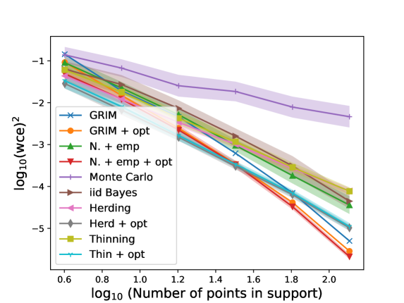
The third and final task we consider is a machine learning inference acceleration task motivated by [JLNSY17]. The problem is outside the Hilbert space framework of the previous examples. We consider the path signature based Landmark Human Action Recognition (LHAR) model developed in [JLNSY17].
This model is trained to determine an action from video clips of the evolution of 15-40 markers placed on a persons body. It utilises signatures of streams generated by the locations of these markers. An introduction to the use of path signatures in machine learning contexts can be found in the survey papers [CK16] and [LM22]. We do not assume any familiarity with signatures and treat them as a ’black box’ tool used by the LHAR model of [JLNSY17].
We restrict consider the LHAR model from [JLNSY17] on the JHMDB data set [BGJSZ13] consisting of 928 clips of 21 distinct actions, with each clip containing 15-40 frames. Following [JLNSY17], the dataset is split into 660 clips to be used for training and 268 clips to be used for testing.
The pipeline for the LHAR model from [JLNSY17] can be summarised as
| (7.6) |
A variety of truncated path signatures are computed of augmentations of the stream of marker locations provided by the clip; see [JLNSY17] for full details. The result is that each clip is transformed into a vector of features, i.e. an element in . Let denote the collection of these vectors for the 660 training clips, and denote the collection of these vectors for the 268 testing clips. A single-hidden-layer neural network is trained as the classifier outputting a probability distribution given by a Softmax over the 21 class labels .
Let denote the Linear Map part of the model in (7.6). For later convenience, given any map we let denote the model from [JLNSY17] with the linear map replaced by (i.e. the pipeline described in (7.6) but with the Linear Map replaced by the function ). We consider approximating the model . Our approach is to find an approximation of , and then use the model as the approximation of . For this purpose, we consider both and to be equipped with their respective norms. We first observe that the task of approximating is within the mathematical framework of this paper.
Let denote the coefficients of the matrix associated to , and for each define by, for , setting . Let be the standard basis of that is orthonormal with respect to the standard Euclidean dot product on . For each and each let be defined by . Then and hence, by choosing , , , and , we observe that we are within the framework for which GRIM is designed (cf. Section 2).
To provide a benchmark we use the Scikit-Learn MultiTaskLasso [BBCDDGGMPPPPTVVW11] implementation to approximate . Several different choices for the regularisation parameter are considered. For each we consider the Scikit-Learn MultiTaskLasso [BBCDDGGMPPPPTVVW11] with the maximum number of iterations set to 10000. We record the number of non-zero weights in the resulting approximation , the training set accuracy achieved by , and the testing set accuracy achieved by . These results are summarised in Table 2.
| Alpha | Number of Non-zero Weights | Train Accuracy (%) (2.d.p) | Test Accuracy (%) (2.d.p) |
|---|---|---|---|
| 0.0001 | 5464 | 100.00 | 81.34 |
| 0.0002 | 4611 | 100.00 | 82.09 |
| 0.0003 | 4217 | 100.00 | 83.21 |
| 0.0004 | 4021 | 100.00 | 82.84 |
| 0.0005 | 4009 | 100.00 | 82.46 |
| 0.001 | 3913 | 100.00 | 82.46 |
| 0.005 | 3157 | 99.70 | 81.72 |
| 0.01 | 2455 | 99.24 | 81.72 |
| 0.05 | 1012 | 95.30 | 79.85 |
In terms of the test accuracy score achieved by the model , the choice of performed best. For this choice of the corresponding model achieved an accuracy score of (2.d.p) on the test set whilst only using 4217 non-zero weights. In comparison, the original model developed in [JLNSY17] uses 430920 non-zero weights, and achieves an accuracy score of (2.d.p) on the test set.
With the Lasso performance acting as a benchmark, we consider applying GRIM to approximate . We consider several choices for the number of new points from to be added to the collection of points over which we require the approximation to coincide with the target . We fix the shuffle number for each step as 16. We apply GRIM to approximate over , i.e. we use only the training set. The test set is not used for constructing the approximation , and is only used to record the accuracy achieved by model generated by the approximation .
We make the following adaptation to the GRIM algorithm for this task. Our aim is to find an approximation of that is close in a pointwise sense to throughout . Instead of considering each linear functional in individually, we consider each collection for a point . We modify the Banach Extension Step (cf. Section 4) to the Modified Extension Step below. Modified Extension Step
Assume that . Let . Let such that . Take
| (7.7) |
Let denote the point for which .
Inductively for take
| (7.8) |
and let denote the point for which .
Once the points have been selected, extend to . Since , we observe that the Modified Extension Step is equivalent to taking
| (7.9) |
then inductively taking for the point
| (7.10) |
and then extending to . Consequently, replacing the Banach Extension Step with the Modified Extension Step in the Banach GRIM algorithm in Section 4 results in an algorithm in which a collection of points, at which we require an approximation of to coincide with , is inductively greedily grown. It is important to keep in mind that each newly selected point corresponds to choosing 21 new linear functionals in . Thus the restriction on the total number of points to possibly be selected is that , which is equivalent to requiring . It is this modification of the Banach GRIM algorithm (cf. Section 4) that we consider for the task of approximating the linear map .
Our aim here is that the model achieves a similar accuracy score as the original model from [JLNSY17]. Consequently, we alter the termination criteria to better reflect this goal. The model from [JLNSY17] achieves an accuracy score of on the test set. We choose and terminate if the approximation generates a model achieving an accuracy score of at least times the accuracy score of the original model on the testing set. Hence we require the approximation to generate a model achieving a testing set accuracy score of at least to 2 decimal places. We further record the accuracy achieved on the training set for comparison with the accuracy achieved by the original model here.
For each choice of number of points to add at each step, we run the GRIM algorithm (modified as outlined above) three times. We record the minimum number of non-zero weights returned after an approximation generating a model with the required test set accuracy score. Subsequently, we record the training accuracy score and testing accuracy score of the models found by each run using this number of non-zero weights. In addition to recording these values for the best performing model, we additionally record the variance of the training accuracy score and testing accuracy score over the three runs. The results are summarised in Table 3 below.
| Points Added | Number of | Train Accuracy (%) | Test Accuracy (%) | ||
|---|---|---|---|---|---|
| Per Step | Non-zero Weights | Best | Variance | Best | Variance |
| 10 | 2101 | 100.00 | 0.04 | 83.58 | 1.12 |
| 20 | 2941 | 100.00 | 0.00 | 83.58 | 0.09 |
| 30 | 2521 | 100.00 | 0.02 | 83.58 | 0.49 |
| 40 | 2521 | 100.00 | 0.01 | 84.33 | 1.33 |
| 50 | 2101 | 99.55 | 0.04 | 83.96 | 0.65 |
For each choice of the number of new points to be added at each step, GRIM successfully finds an approximation of which is both uses fewer non-zero weights than the best performing model found via Lasso, and achieves a higher test accuracy score than the best performing model found via Lasso. The best performance, in terms of accuracy score on the test set, was achieved by GRIM with the choice of adding 40 new points at each step. The best performing model uses 2521 non-zero weights and achieves an accuracy score of (2.d.p) on the test set. This accuracy score is actually higher than the accuracy score of (2.d.p) achieved by the original model from [JLNSY17] on the test set.
References
- [ACO20] A. Abate, F. Cosentino, and H. Oberhauser, A randomized algorithm to reduce the support of discrete measures, In Adavances in Neural Information Processing Systems, Volume 33, pages 15100-15110, 2020.
- [ABDHP21] D. Alistarh, T. Ben-Nun, N. Dryden, T. Hoefler and A. Peste, Sparsity in Deep Learning: Pruning and growth for efficient inference and training in neural networks, J. Mach. Learn. Res., 22(241), 1-124, 2021.
- [ABCGMM18] J.-P. Argaud, B. Bouriquet, F. de Caso, H. Gong, Y. Maday and O. Mula, Sensor Placement in Nuclear Reactors Based on the Generalized Empirical Interpolation Method, J. Comput. Phys., vol. 363, pp. 354-370, 2018.
- [ABGMM16] J.-P. Argaud, B. Bouriquet, H. Gong, Y. Maday and O. Mula, Stabilization of (G)EIM in Presence of Measurement Noise: Application to Nuclear Reactor Physics, In Spectral and High Order Methods for Partial Differential Equations-ICOSAHOM 2016, vol. 119 of Lect. Notes Comput. Sci. Eng., pp.133-145, Springer, Cham, 2017.
- [AK13] M. G. Augasts and T. Kathirvalavakumar, Pruning algorithms of neural networks - A comparative study, Open Computer Science 3, p.105-115, 2013.
- [BLL15] Francis Bach, Simon Lacoste-Julien and Fredrik Lindsten, Sequential Kernel Herding: Frank-Wolfe Optimization for Particle Filtering, In Artificial Intelligence and Statistics, pages 544-552, PMLR, 2015.
- [BMPSZ08] F. R. Bach, J. Mairal, J. Ponce, G. Sapiro and A. Zisserman, Discriminative learned dictionaries for local image analysis, Compute Vision and Pattern Recognition (CVPR), pp.1-8, IEEE 2008.
- [BMPSZ09] F. R. Bach, J. Mairal, J. Ponce, G. Sapiro and A. Zisserman, Supervised dictionary learning, Advances in Neural Information Processing Systems, pp.1033-1040, 2009.
- [BMNP04] M. Barrault, Y. Maday, N. C. Nguyen and A. T. Patera, An Empirical Interpolation Method: Application to Efficient Reduced-Basis Discretization of Partial Differential Equations, C. R. Acad. Sci. Paris, Série I., 339, pp.667-672, 2004
- [BS18] A. G. Barto and R. S. Sutton, Reinforcement learning: an introduction, (2nd). Cambridge, MA, USA: MIT Press.
- [BT11] Alain Belinet and Christine Thomas-Agnan, Reproducing kernel Hilbert spaces in probabiility and statistics, Springer Science & Business Media, 2011.
- [BBCDDGGMPPPPTVVW11] M. Blondel, M. Brucher, D. Cournpeau, V. Dubourg, E. Duchesnay, A. Gramfort, O. Grisel, V. Michel, A. Passos, F. Pedregosa, M. Perrot, P. Prettenhofer, B. Thirion, J. Vanderplas, G. Varoquax and R. Weiss, Scikit-learn: Machine Learning in Python, Journal of Machine Learning Research, 12, 2825-2830, 2011.
- [BCGMO18] F. -X. Briol, W. Y. Chen, J. Gorham, L. Mackey and C. J. Oates, Stein Points, In Proceedings of the 35th International Conference on Machine Learning, Volume 80, pp. 843-852, PMLR, 2018.
- [BGJSZ13] J. Black, J. Gall, H. Jhuang, C. Schmid and S. Zuffi, Towards understanding action recognition, In IEEE International Conference on Computer Vision (ICCV), pp. 3192-3199, 2013.
- [CT05] E. Candés and T. Tao, Decoding by linear programming, IEEE Trans. Inform. Theory, 51, 2005.
- [CRT06] E. Candés, J. Romberg and T. Tao, Robust Uncertainty Principles: Exact Signal Reconstruction from Highly Incomplete Frequency Information, IEEE Trans. Inform. Theory, 52, pp. 489-509, 2006.
- [Car81] B. Carl, Entropy numbers of diagonal operators with an application to eigenvalue problems, J. Approx. Theory, 32, pp.135-150, 1981.
- [CS90] B. Carl and I. Stephani, Entropy, Compactness, and the Approximation of Operators, Cambridge University Press, Cambridge, UK, 1990.
- [CHXZ20] L. Chen, A. Huang, S. Xu and B. Zhang, Convolutional Neural Network Pruning: A Survey, 39th Chinese Control Conference (CCC), IEEE, p.7458-7463, 2020.
- [CSW11] Zhixiang Chen, Baohuai Sheng and Jianli Wang, The Covering Number for Some Mercer Kernel Hilbert Spaces on the Unit Sphere, Taiwanese J. Math. 15(3), p.1325-1340, 2011.
- [CSW10] Y. Chen, A. Smola and M. Welling, Super-Samples from Kernel Herding, In Proceedings of the Conference on Uncertainty in Artificial Intelligence, 2010.
- [CS08] A. Christmann and I. Steinwart, Support Vector Machines, Springer Science & Business Media, 2008.
- [CM73] Jon F. Claerbout and Francis Muir, Robust Modeling with Erratic Data, Geophysics, Vol. 38, So. 5, pp. 826-844, (1973)
- [CK16] Ilya Chevyrev and Andrey Kormilitzin, A Primer on the Signature Method in Machine Learning, arXiv preprint, 2016. https://arxiv.org/abs/1603.03788
- [DGOY08] J. Darbon, D. Goldfarb, S. Osher and W. Yin, Bregman Iterative Algorithms for L1 Minimization with Applications to Compressed Sensing, SIAM J. Imaging Sci. 1, pp.143-168, 2008.
- [Don06] D. Donoho, Compressed Sensing, IEEE Trans. Inform. Theory, 52, pp. 1289-1306, 2006.
- [DE03] D. Donoho and M. Elad, Optimally Sparse Representation in General (Nonorthogonal) Dictionaries via Minimization, Proc. Natl. Acad. Sci. USA, 100, pp.2197-2202, 2003.
- [DET06] D. L. Donoho, M. Elad and V. Templyakov, Stable recovery of sparse overcomplete representations in the presence of noise, IEEE Transactions on Information Theory, 52(1): 6-18, 2006.
- [DM21a] Raaz Dwivedi and Lester Mackey, Kernel Thinning, Proceedings of Machine Learning Research vol. 134:1–1, 2021.
- [DM21b] Raaz Dwivedi and Lester Mackey, Generalized Kernel Thinning, Published in ICLR 2022.
- [DMS21] Raaz Dwivedi, Lester Mackey and Abhishek Shetty, Distribution Compression in Near-Linear Time, Published in ICLR 2022.
- [DF15] Chris Dyer and Manaal Faruqui, Non-distributional Word Vector Representations, Proceedings of the 53rd Annual Meeting of the Association for Computational Linguistics and the 7th International Joint Conference on Natural Language Processing, Association for Computational Linguistics, Beijing, China, Volume 2: Short Papers, pp.464-469, 2015.
- [ET96] D. E. Edmunds and H. Triebel, Function Spaces, Entropy Numbers, and Differential Operators, Cambridge University Press, Cambridge, UK, 1996.
- [Ela10] M. Elad, Sparse and Redundant Representations: From Theory to Applications in Signal and Image Processing, Springer, ISBN 978-1441970107, 2010.
- [EMS08] M. Elad, J. Mairal and G. Sapiro, Sparse representation for color image restoration, IEEE Transactions on Image Processing, 17(1), 53-69, 2008.
- [EJOPR20] E. Elsen, S. Jayakumar, S. Osindere, R. Pascanu and J. Rae, Top-kast: Top-k always sparse training, Advances in Neural Information Processing Systems, 33:20744-20754, 2020.
- [EPP00] T. Evgeniou, M. Pontil and T. Poggio, Regularization networks and support vector machines, Adv. Comput. Math., 13, pp.1-50, 2000.
- [FHLLMMPSWY23] Meng Fang, Tianjin Huang, Gen Li, Shiwei Liu, Xiaolong Ma, Vlado Menkovski, Mykola Pechenizkiy, Li Shen, Zhangyang Wang and Lu Yin, Dynamic Sparsity in Channel-Level Sparsity Learner, NeurIPS 2023.
- [FJM19] Dan Feldman, Ibrahim Jubran and Alaa Maalouf, Fast and Accuract Least-Mean-Squares Solvers, Advances in Neural Information Processing Systems 32 (NeurIPS2019), 2019.
- [FJM22] Dan Feldman, Ibrahim Jubran and Alaa Maalouf, Fast and Accurate Least-Mean-Squares Solvers for High Dimensional Data, in IEEE Transactionf on Pattern Analysis and Machine Intelligence, vol. 44, no. 12, pp. 9977-9994, 2022.
- [FS21] S. Fischer and I. Steinwart, A closer look at covering number bounds for Gaussian kernels, Journal of Complexity, Volume 62, 2021.
- [FMMT14] Alona Fyshe, Tom M. Mitchell, Brian Murphy and Partha P. Talukdar, Interpretable semantic Vectors from a joint model of brain-and text-based meaning, Proceedings of the 52nd Annual Meeting of the Association for Computational Linguistics, Association for Computational Linguistics, Baltimore, Maryland, Volume 1: Long Papers, pp.489-499, 2014.
- [GMSWY09] A. Ganesh, Y. Ma, S. S. Sastry, J. Wright and A. Yang, Robust face recognition via sparse representation, TPAMI 31(2), 210-227, 2009.
- [GLMNS18] M. Gibescu, A. Liotta, D. C. Mocanu, E. Mocanu, P. H. Nguyen and P. Stone, Scalable training of artificial neural networks with adaptive sparse connectivity inspired by network science, Nature communications, 9(1):2383, 2018.
- [GLSWZ21] John Glossner, Tailin Liang, Shaobo Shi, Lei Wang and Xiaotong Zhang, Pruning and quantization for deep neural network acceleration: A survey, Neurocomputing, Volume 461, pages 370-403, 2021.
- [GO09] T. Goldstein and S. Osher, The Split Bregman Method for L1-Regularized Problems, SIAM J. Imaging Sci. 2, pp.323-343, 2009.
- [GMNP07] M. A. Grepl, Y. Maday, N. C. Nguyen and A. T. Patera, Efficient Reduced-Basis Treatment of Nonaffine and Nonlinear Partial Differential Equations, M2AN (Math. Model. Numer. Anal.), 2007.
- [GKT12] F. S. Gürgen, H. Kaya and P. Tüfekci, Local and global learning methods for predicting power of a combined gas & steam turbine, In Proceedings of the Internationl Conference on Emerging Trends in Computer and Electronics Engineering, pages 13-18, 2012.
- [HLO21] Satoshi Hayakawa, Terry Lyons and Harald Oberhauser, Positively weighted kernel Quadrature via Subsampling, In Adavnces in Neural Information Processing Systems (NeurIPS 2022).
- [HS19] J. Hernandez-Garcia and R. Sutton, Learning Sparse Representations Incrementally in Deep Reinforcement Learning, https://arxiv.org/abs/1912.04002, [cs.LG], 9 Dec 2019.
- [HLLL18] J. Huang, H. Lian, H. Lin and S. Lv, Oracle Inequalities for Sparse Additive Quantile Regression in Reproducing Kernel Hilbert Space, Annals of Statistics 46, p.781-813, 2018.
- [JLPST21] S. Jayakumar, P. E. Latham, R. Pascanu, J. Schwarz and Y. Teh, Powerpropagation: A sparsity inducing weight reparameterisation, Advances in Neural Information Processing Systems, 34:28889-28903, 2021.
- [JKY13] C. S. Jensen, M. Kaul and B. Yang, Building accurate 3d spatial networks to enable next generation intelligent transportation systems, In 2013 IEEE 14th International Conference on Mobile Data Management, Volume 1, pages 137-146, IEEE, 2013.
- [JJWWY20] C. Jin, M. I. Jordan, M. Wang, Z. Wang and Z. Yang, On Function Approximation in Reinforcement Learning: Optimism in the Face of Large State Spaces, 34th Conference on Neural Information Processing Systems (NeurIPS 2020), Vancouver, Canada, 2020
- [JLNSY17] Lianwen Jin, Terry Lyons, Hao Ni, Cordelia Schmid and Weixin Yang, Developing the Path Signature Methodology and its Application to Landmark-based Human Action Recognition, In: Yin, G., Zariphopoulou, T. (eds) Stochastic Analysis, Filtering and Stochastic Optimization, Springer, Cham. 2022. https://doi.org/10.1007/978-3-030-98519-6_18
- [KK20] M. Kalinić and P. Kómár, Denoising DNA encoded library screens with sparse learning, ACS Combinatorial Science, Vol. 22, no. 8, pp.410-421, 2020.
- [Kol56] A. N. Kolmogorov, Asymptotic characteristics of some completely bounded metric spaces, Dokl. Akad. Nauk. SSSR, 108, pp.585-589, 1956.
- [Kuh11] T. Kühn, Covering numbers of Gaussian reproducing kernel Hilbert spaces, J. Complexity, 27, pp.489-499, 2011.
- [LY07] Y. Lin and M. Yuan, On the Non-Negative Garrote Estimator, J. R. Stat. Soc. Ser. B 69, pp. 143-161, 2007
- [LL16] W. Lee and T. Lyons, The Adaptive Patched Cubature Filter and its Implementation, Communications in Mathematical Sciences, 14(3), pp.799-829, 2016.
- [LL99] W. V. Li and W. Linde, Approximation, metric entropy and small ball estimates for Gaussian measures, Ann. Probab., 27, pp.1556-1578, 1999.
- [LL12] C. Litterer and T. Lyons, High order recombination and an application to cubature on wiener space, The Annals of Applied Probability, Vol. 22, No. 4, 1301-1327, 2012.
- [LMPY21] S. Liu, D. C. Mocanu, M. Pechenizkiy and L. Yin, Do we actually need dense over-parameterization? in-time over-parameterization in sparse training, In Proceedings of the International Conference on Machine Learning, pages 6989-7000, PMLR 2021.
- [LP04] H. Luschgy and G. Pagés, Sharp asymptotics of the Kolmogorov entropy for Gaussian measures, J. Funct. Anal., 212, pp.89-120, 2004.
- [LM22] Terry Lyons and Andrew D. McLeod, Signature Methods in Machine Learning, arXiv preprint, 2022. https://arxiv.org/abs/2206.14674
- [MM13] Y. Maday, O. Mula, A generalized empirical interpolation method: Application of reduced basis techniques to data assimilation, F. Brezzi, P. Colli Franzone, U. Gianazza, G. Gilardi (Eds.), Analysis and Numerics of Partial Differential Equations, Vol. 4 of Springer INdAM Series, Springer Milan, 2013, pp. 221–235.
- [MMPY15] Y. Maday, O. Mula, A. T. Patera and M. Yano, The Generalized Empirical Interpolation Method: Stability Theory On Hilbert Spaces With An Application To Stokes Equation, Comput. Methods Appl. Mech. Engrg. 287, 310-334, 2015.
- [MMT14] Y. Maday, O. Mula and G. Turinici, Convergence analysis of the Generalized Empirical Interpolation Method, SIAM J. Numer. Anal., 54(3) 1713-1731, 2014.
- [MNPP09] Y. Maday, N. C. Nguyen, A. T. Patera and G. S. H. Pau, A General Multipurpose Interpolation Procedure: The Magic Points, Commun. Pure Appl. Anal., 81, pp. 383-404, 2009.
- [MZ93] S. G. Mallat and Z. Zhang, Matching Pursuits with Time-Frequency Dictionaries, IEEE Transactions on Signal Processing, 12: 3397-3415, 1993.
- [MRT12] Mehryar Mohri, Afshin Rostamizadeh and Ameet Talwalkar, Foundations of Machine Learning, Massachusetts: MIT Press, USA, 2012
- [NT09] D. Needell and J. A. Tropp, CoSaMP: Iterative signal recovery from incomplete and inaccurate samples, Applied and Computational Harmonic Analysis, 26(3): 301-321, 2009.
- [NPS22] M. Nikdast, S. Pasricha and F. Sunny, SONIC: A Sparse Neural Network Inference Accelerator with Silicon Photonics for Energy-Efficient Deep Learning, 27th Asia and South Pacific Design Automation Conference (ASP-DAC), pp. 214-219, 2022.
- [NS21] S. Ninomiya and Y. Shinozaki, On implementation of high-order recombination and its application to weak approximations of stochastic differential equations, In Proceedings of the NFA Annual Conference, 2021.
- [PTT22] Sebastian Pokutta, Ken’ichiro Tanaka and Kazuma Tsuji, Sparser Kernel Herding with Pairwise Conditional Gradients without Swap Steps, https://arxiv.org/abs/2110.12650, [math.OC], 8 February 2022.
- [Ree93] R. Reed, Pruning Algorithms - A Survey, IEEE Transactions on Neural Networks 4, p.74-747, 1993.
- [SS86] Fadil Santosaf and William W. Symes, Linear Inversion of Band-Limited Reflection Seismograms, SIAM J. ScI. STAT. COMPUT. Vol. 7, No. 4, 1986.
- [SSW01] B. Schölkopf, A. J. Smola and R. C. Williamson, Generalization performance of regularization networks and support vector machines via entrop numbers of compact operators, IEEE Trans. Inform. Theory, 47, pp.2516-2532, 2001.
- [Ste03] I. Steinwart, Entropy numbers of convex hulls and an application to learning algorithms, Arch. Math., 80, pp.310-318, 2003.
- [SS07] I. Steinwart and C. Scovel, Fast rates for support vector machines using Gaussian kernels, Ann. Statist. 35 (2), 2007.
- [SS12] I. Steinwart and C. Scovel, Mercer’s theorem on general domains: On the interaction between measures, kernels, and RKHSs, Constructive Approximation, 35(3):363-417, 2012.
- [Str71] A. H. Stroud, Approximate calculation of multiple integrals, Series in Automatic Computation, Englewood Cliffs, NJ: Prentice-Hall, 1971.
- [Suz18] T. Suzuki, Fast Learning Rate of Non-Sparse Multiple Kernel Learning and Optimal Regularization Strategies, Electronic Journal of Statistics 12, p.2141-2192, 2018.
- [SS13] M. Sugiyama and T. Suzuki, Fast Learning Rate of Multiple Kernel Learning: Tradeoff Between Sparsity and Smoothness, Annals of Statistics 41, p.1381-1405, 2013.
- [TT21] Ken’ichiro Tanaka and Kazuma Tsuji, Acceleration of the Kernel Herding Algorithm by Improved Gradient Approximation, https://arxiv.org/abs/2105.07900, [math.NA], 17 May 2021.
- [Tch15] M. Tchernychova, Carathéodry cubature measures, PhD thesis, University of Oxford, https://ora.ox.ac.uk/objects/uuid:a3a10980-d35d-467b-b3c0-d10d2e491f2d 2015.
- [TW19] GL. Tian and M. Wang, Adaptive Group LASSO for High-Dimensional Generalized Linear Models, Stat Papers 60, pp. 1469-1486, 2019.
- [Tib96] Robert Tibshirani, Regression Shrinkage and Selection via the Lasso, Journal of the Royal Statistical Society. Series B (Methodological), Vol. 58, No. 1, pp. 267-288, 1996.
- [Tro06] J. A. Tropp, Just relax: Convex programming methods for identifying sparse signals in noise, IEEE Transactions on Information Theory, 52(3): 1030-1051, 2006.
- [Wel09a] M. Welling, Herding Dynamical Weights to Learn, In Proceedings of the 21st International Conference on Machine Learning, Montreal, Quebec, CAN, 2009.
- [Wel09b] M. Welling, Herding Dynamic Weights for Partially Observed Random Field Models, In Proc. of the Conf. on Uncertainty in Artificial Intelligence, Montreal, Quebec, CAN, 2009.
- [XZ16] Y. Xiang and C. Zhang, On the Oracle Property of Adaptive Group LASSO in High-Dimensional Linear Models, Stat. Pap. 57, pp. 249-265, 2016.
- [Zho02] D. -X. Zhou, The covering number in learning theory, J. Complexity, 18, pp.739-767, 2002.
University of Oxford, Radcliffe Observatory,
Andrew Wiles Building, Woodstock Rd, Oxford,
OX2 6GG, UK.
TL: [email protected]
https://www.maths.ox.ac.uk/people/terry.lyons
AM: [email protected]
https://www.maths.ox.ac.uk/people/andrew.mcleod