Gravitational Waves with Dark Energy
Abstract
In this article, we study the tensor mode equation of perturbation in the presence of nonzero as dark energy, the dynamic nature of which depends on the Hubble parameter and/or its time derivative. Dark energy, according to the total vacuum contribution, has a slight effect during the radiation-dominated era, but it reduces the squared amplitude of gravitational waves (GWs) up to for the wavelengths that enter the horizon during the matter-dominated era. Moreover, the observations bound on dark energy models, such as running vacuum model (RVM), generalized running vacuum model (GRVM) and generalized running vacuum subcase (GRVS), are effective in reducing the GWs’ amplitude. Although this effect is less for the wavelengths that enter the horizon at later times, this reduction is stable and permanent.
pacs:
98.80.-k, 04.20.Cv, 02.40.-kIntroduction
Primordial gravitational waves (GWs; or tensor mode perturbations) arise from inflationary at early times and propagate freely to the expanding universe without any interactions with the matter and radiation Lifshitz ; Mukhanov . However, it is shown that at the temperature of , the tensor modes can be affected by anisotropic inertia, which contains free streaming neutrinos and antineutrinos damping . This issue has been explored in the spatially curved spacetime and extended to the -dominated era Khodagholizadeh:2014ixa ; Khodagholizadeh:2017ttk ; khoda . Here, we study the effect of dark energy on GWs.
Current observational data indicate that the dark energy is a cosmological constant without evidence for its conclusiveness 126 ; 128 ; 130 ; 132 ; 133 ; 134 ; 136 ; 137 ; 143 ; 145 ; 146 . Moreover, dark energy is one of the most compelling mysteries, which is thought to be behind the present cosmic acceleration Riess ; Perl .
The dynamic nature of could be conventionally achieved in three models: the first model has an explicit function of time, in which the most popular relation is in the form of the inverse power law as 44 ; 45 ; 46 ; 47 ; 48 , and the other in this category is proposed as an exponential decay 52 . The next model could be expressed in terms of the scale factor , in which the general form is or the relation consistent with the data is . In spatially flat cosmology, shows consistency with lensing data 63 , while is the framework of the closed cosmology with the condition that matter/radiation densities are equal to the critical density at all times 65 . The third class of expressions for is based on the Hubble parameter as the usual function of and , in which is disqualified by cosmic microwave background (CMB) data 74 . A general form of this model is known as the generalized running vacuum model (GRVM):
| (1) |
Here, dot denotes the differentiation with respect to cosmic time.
and are constants and dimensionless, and has the unit of length-2. A classical running vacuum model (RVM) 24 ; 25 ; 26 ; 27 ; 28 is a null value for . Both RVM and GRVM appear to provide a better fit to the structure formation data sola1 ; sola2 ; sola3 . We shall refer to the latter as the generalized running vacuum subcase (GRVS) with , which was investigated in ref.30 as a model with a variable dark energy equation-of-state parameter. Here, we assumed that the equation-of-state parameter of dark energy, , is fixed at -1, similar to CDM. In the following, we study the effect of the three models on GWs.
This paper is organized as follows. In Sec. II, we derive the equation of the tensor mode perturbation in the presence of as dark energy. In the next Sections, the solutions of the mentioned equation are studied separately in all the cosmic history. Finally, the results are reported.
Linear field equation with dynamic dark energy
Let’s decompose the perturbed metric as:
| (2) |
where is the background metric and is the symmetric perturbation term with the condition . The metric components of the Friedmann–Lemaitre–Robertson–Walker (FLRW) model in the Cartesian coordinate system are 1 :
| (3) |
with and running over the values 1, 2 and 3; is the time coordinate in our units, the speed of light is equal to unity and is the curvature constant. Also, is the scale factor, which will be and in the closed de Sitter spacetime. From Pad , the field equation for the tensor mode fluctuation in the source free region is:
| (4) |
where is the background Riemann tensor. This equation describes the propagation of weak GWs in the source-free region of the curved spacetime. If the amplitude and the wavelength of are and , in the above relation, the first term is in the order of and the second term is while is the scale over which the background geometry is varied. Hence, in the order of , we can ignore the second term and the well-known GW equation will be:
| (5) |
For calculating, the metric can be put in the form of where s are the functions of and , satisfying the traceless-transverse conditions (or TT gauge):
| (6) |
These conditions are used to obtain Eq.(4). With manipulation calculations shown in Appendix A, we can show that:
| (7) | |||||
Moreover, one can show with straightforward calculations that:
| (8) | |||||
By using the above expression and the Friedmann equation, , in which the cosmological constant is of dynamic nature, Eq.(5) will be:
| (9) |
By looking at the plane-wave analogue and without losing generality, we chose the solution of the above equation as a move in the direction. Therefore, by using the modified transverse and traceless conditions, with some manipulation, we conclude that each mode, and , holds true in the following relation (e.g., in closed spacetime, ; please see Relations (29) and (30) in Ref.Khodagholizadeh ).
| (10) |
With the method of separation of variables , the time evolution of the tensor mode perturbation will be:
| (11) |
where in which is a wavenumber. If the space-time background is curved, the wavenumber must be discrete, which comes from examining the periodic solution of the spatial part of the wave equation Khodagholizadeh . Therefore, the final time evolution of GWs in the presence of as dark energy will be:
| (12) |
The expression is also a wavenumber. It should be noted that, in Eq. (4), the presence of the second term results in the expression , in which the value 2 is added to the discrete wavenumber .
Here, we have both the spatially curvature parameter and the cosmological constant. It seems the nonzero curvature has an effect on constraining some dark energy models Polarski ; Franca ; Ichikawa ; Ichikawa1 ; Clarkson ; Gong ; Ichikawa2 ; Wright ; Zhao . Using CMB, type Supernova Ia (SNe Ia) and galaxy survey data show that the bounds on cosmic curvature are less stringent if dark energy density is allowed to be free of redshift and are dependent on the assumption about its early time properties. However, assuming a constant dark energy equation of state gives the most stringent constraints on cosmic curvatureWang:2007mza . Nevertheless, for all the values of the curvature parameter, term has an important role in the evolution of the GWs.
In the next section, the treat of Eq.(12) is studied in the radiation-dominated era.
Effect of running vacuum model in radiation-dominated era
The parameters and/or are constrained by means of an Markov chain Monte Carlo (MCMC) analysis, initially using data for the observables associated with SNe Ia, cosmic chronometers, CMB and baryon acoustic oscillations (BAOs) Farrugia:2018mex . At early times the Eq.(1) is no longer valid because the density of dark energy ’blows up’ (it decays with time, so if you extend the model too far back, you get unrealistically large quantities). On the other hand, it is better to use a more general model. The total vacuum contribution or the RVM with its generalized version takes spatial curvature into account after inflation is described in the complete cosmic history as Lima:2015kda .
| (13) |
where and stand for the Hubble parameter in two different epochs, while the former characterizes inflation, the latter denotes the final value of H as . Also, is the limit of as . Although rather generally, the above expression can be simplified based on different arguments. First, without loss of generality, we can see that parameter can be absorbed in the value of the scale , so that we may fix and, with this condition, there is no fluid component; therefore, we have . Another reason is that is expected to be already much smaller than at the beginning of adiabatic radiation phase and so the constant term dominates with the model following evolutionLima:2015kda . Since we are not concerned with inflation, but rather with the late time behavior of dark energy models, the term may therefore be dropped and the resulting cosmology converge to . Moreover, in a flat case, S. Basilakos et. al Basil obtained based on a joint analysis involving CMB, SNe Ia and BAO, while a theoretical analysis by J. Sola Sola yielded within a generic grand unified theory (GUT). Therefore, since the curvature must be very small nowadays, can be assumed for all values of the curvature. With the above explanations, assuming the simplest form in the radiation-dominated phase, in which dark energy is coupled to the matter, we have:
| (14) |
As mentioned, is the value of the running when ; thus, it can be neglected at early times; therefore, with and the above expression, Eq. (12) will be:
| (15) |
To investigate the treat of the tensor mode in the radiation- and matter-dominated eras, it is convenient to change the independent variable to . By using the Friedmann equation , and as the scale factor in the radiation-dominated era, Eq. (15) becomes
| (16) |
Generally, tensor mode perturbation rapidly becomes time-independent after the horizon exit and remains so until horizon re-entry; thus, there are initial conditions:
| (17) |
For deep inside the horizon, Eq. (16) approaches a solution as:
| (18) |
where and are the spherical Bessel functions of the first and second kinds, respectively. By using the definition of spherical Bessel functions, and , the general solution is:
| (19) |
The coefficient of the second term must be zero; so, . In addition, for large , the tensor modes are deep inside the horizon and the solution has to approach the homogeneous solution; thus, . Therefore, the final solution will be:
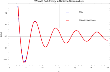
| (20) |
The second term, which is due to the presence of dark energy, is very smaller than the first term. As shown in Fig.1, it has a slight effect on reducing the amplitude of GWs in the radiation-dominated era, so it can be ignored.
Short wavelengths in matter-dominated era
For the more detailed study of GWs in the presence of dark energy in the matter-dominant era, using the definition , where , the equation of the tensor mode time evolution will be:
| (21) |
The general solution is based on the Bessel functions of the first and second kinds as:
| (22) |
where and are constant. At the moment that the perturbations enter the horizon, , the solution tends toward the solution of homogeneous equation; thus, it will be:
| (23) |
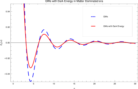
where is the cosine integral as . Deep inside the horizon, when , the right hand side of Eq. (21) becomes negligible and the solution approaches a homogeneous solution as . Because large , and the third term of the general solution tend toward zero, . As compared with the solution in the absence of dark energy, Eq. (21) shows that follows the without dark energy solution rather accurately until , when the perturbation enters the horizon and, thereafter, rapidly approaches , in which is very small and negligible. Furthermore, it has a significant effect on decreasing the B-B polarization multipole coefficient, , which is up to less than it would be without the damping due to dark energy (see Fig. 2).
As mentioned earlier, the constant parameters of RVM, GRVM and GRVS are obtained using the combination of type-Ia supernova, cosmic chronometers, BAO and CMB Farrugia:2018mex . The results are based on the data sets which are in the framework of cosmology with freely varying and are valid Until near the end of matter-dominated era. A general form of the GW equation with the mentioned models will be:
| (24) |
The largest constant obtained based on models for RVM is ; for GRVM, it is and ; for GRVS, the biggest coefficient is Farrugia:2018mex .
For GRVM, RVM and GRVS, the numerical solutions of (24), which are deep inside the horizon, are , and , respectively. Thus, the dark energy decreases the B-B polarization multipole coefficient, , up to , and , respectively, less than it would be without the damping due to dark energy. Therefore, the effect of dark energy on reducing the amplitude will be less when the expression is larger.
In other words, the effect of dark energy on cosmological GWs will be greater if, in all theories, the value of is higher or the value of is lower.
General wavelengths in the dark energy-dominated era
After , the universe begins to accelerate and the dark energy is dominated Frieman:2008sn . To investigate tensor mode perturbation, it is convenient to change the independent variable to
where , and are the value of the Robertson-Walker scale factor, energy densities of vacuum and matter at matter-vacuum equality. Moreover, we have . and are the Hubble rate and the redshift at matter-vacuum equality, respectively.
In the condition , when the dark energy is important, according to the Friedmann equation, we have:
| (25) |
where is the curvature density at matter-vacuum equality. Thus, the homogeneous equation of GWs in the expansion universe will be:
| (26) |
where is the dimensionless rescaled wavenumber:
| (27) |
Due to the very small value of , e.g., with Planck:2015fie , we can ignore it. Therefore:
| (28) |
where is the present-day scale factor.
In the cases of long and short wavelengths, we have and , respectively, and the cosmological GWs are detectable when .
Recently, the existing ground-based operators, LIGO and VIRGO, reported GWs that are coming from black-hole mergers GWs . These detectors do not have sensitivity to detect cosmological GWs; thus, they might be detected by space-borne laser interferometers, which operate at frequencies around to Hz. Therefore, GWs with the observed frequency of Hz Komatso would have at the present epoch.
The damping effect is small in any way for ; so, it will be adequate approximation for all the wavelengths to take the solution of Eq. (26) in the -dominated era to be given by multiplying by a factor :
| (29) |
where in GRVM which is the biggest reduction. For , we have and in , the above relation will be:
| (30) |
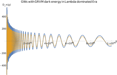
All the observable effects of primordial gravitational waves will be reduced by these factors of dark energy models. When a GW enters the horizon, it has short wavelength, but deep inside the horizon, it will take similar long wavelength (see Fig. 3 Left).
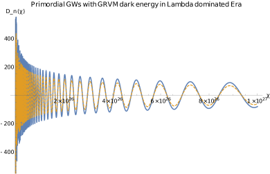
If the frequency sensitivity of the detector is of Hz which is able to observe the primordial gravitational waves coming from the quark-gluon plasma phase transition, then, . However, in the dark energy-dominated era, unlike the previous eras, such as the radiation and matter eras, this amplitude reduction which is due to dark energy relatively affects the long wavelengths (see the right plot in Fig. 3 ).
Conclusion
In all scales and at all times, dark energy is present alongside GWs after the inflation epoch. Its minimum effect is seen in the radiation-dominated era, in which its solution will be in terms of multiplied by the spherical Bessel functions. In the matter-dominated era, according to the total vacuum contribution, we will have the maximum GW reduction as , but in the near end of its epoch, by using dark energy models such as RVM, GRVM and GRVS, the highest reduction is and selecting the values of and is effective in the range of reduction. Hence, all the quadratic effects of the tensor modes in the CMB, such as tensor contribution to the temperature multipole coefficients and all of the B-B polarization multipole coefficients, are less than they would be in the case without the damping due to dark energy terms with total vacuum contribution. The maximum reduction for polarization multipole coefficients is observed in the GRVM, which is .
In the dark energy-dominated era, unlike the epoch of the radiation- and matter-dominated eras, in which the effect of dark energy on GWs is destroyed at long wavelengths, this effect always exists and the amplitude reduction is stable. Also, the accommodation of nonzero spatial curvature with dark energy has almost no effect on GWs.
Appendix A
For calculating the we have
| (31) | |||||
From the background metric (3) in addition to the perturbed metric, , the first term will be :
The second term will be
The third term will be
| (34) | |||||
and the fourth term will be
The tensor mode perturbation to the metric can be put in the form which and , where s are functions of and , satisfying the traceless-transverse conditions (or TT gauge):
| (36) |
Therefore with manipulation calculations by the summation of relations (Appendix A), (Appendix A),(34) and (Appendix A) we have
| (37) | |||||
Then
| (38) | |||||
Also one can show with straightforward calculations
| (39) | |||||
By using above expression and the Friedmann equation, in which cosmological constant has a dynamic nature, the Eq.(5) will be
| (40) |
References
- (1) E. M. Lifshitz, Zh. Eksp. Teor. Phys. 16,587 (1946) ; L.P. Grishchuk, Zh .Eksp. Teor. Fiz. 67 ,825 (1974)[Sov. Phys.JETP 40,409(1975)]; L. H. Ford and L. Parker, Phys. Rev. D 16.1601 (1977)
- (2) V. F. Mukhanov, H.A. Feldman, and R. H. Brandenberger, Physics Reports 215, 203 (1992); M. S. Turner, M. White and J. E. Lidsey, Phys. Rev. D 48, 4613 (1993); M. S. Turner, Phys Rev. D. 55, 435 (1997); D. J. Schwarz, astro-ph/0303574. [arXiv:1605.06312 [physics.gen-ph]].
- (3) S. Weinberg, “Damping of tensor modes in cosmology,” Phys. Rev. D 69, 023503 (2004). [astro-ph/0306304].
- (4) J. Khodagholizadeh, A. H. Abbassi and A. A. Asgari, “Damping of tensor mode in spatially closed cosmology,” Phys. Rev. D 90, no.6, 063520 (2014) [arXiv:1409.6958 [astro-ph.CO]].
- (5) J. Khodagholizadeh, A. H. Abbassi and A. A. Asgari, “Damping of gravitational waves in matter and dominated era,” Astropart. Phys. 95, 1-5 (2017).
- (6) J. Khodagholizadeh, “Neutrinos as a probe of curvature,” JHEAp 32 (2021), 20-27 doi:10.1016/j.jheap.2021.08.002 [arXiv:2108.11423 [gr-qc]].
- (7) Y. Wang and M. Tegmark, “New dark energy constraints from supernovae, microwave background and galaxy clustering,” Phys. Rev. Lett. 92, 241302 (2004) doi:10.1103/PhysRevLett.92.241302 [arXiv:astro-ph/0403292 [astro-ph]].
- (8) U. Alam and V. Sahni, “Confronting braneworld cosmology with supernova data and baryon oscillations,” Phys. Rev. D 73, 084024 (2006) doi:10.1103/PhysRevD.73.084024 [arXiv:astro-ph/0511473 [astro-ph]].
- (9) H. K. Jassal, J. S. Bagla and T. Padmanabhan, “Observational constraints on low redshift evolution of dark energy: How consistent are different observations?,” Phys. Rev. D 72, 103503 (2005) doi:10.1103/PhysRevD.72.103503 [arXiv:astro-ph/0506748 [astro-ph]].
- (10) V. Barger, Y. Gao and D. Marfatia, “Accelerating cosmologies tested by distance measures,” Phys. Lett. B 648, 127-132 (2007) doi:10.1016/j.physletb.2007.03.021 [arXiv:astro-ph/0611775 [astro-ph]].
- (11) J. Dick, L. Knox and M. Chu, “Reduction of cosmological data for the detection of time-varying dark energy density,” JCAP 07, 001 (2006) doi:10.1088/1475-7516/2006/07/001 [arXiv:astro-ph/0603247 [astro-ph]].
- (12) D. Huterer and H. V. Peiris, “Dynamical behavior of generic quintessence potentials: Constraints on key dark energy observables,” Phys. Rev. D 75, 083503 (2007) doi:10.1103/PhysRevD.75.083503 [arXiv:astro-ph/0610427 [astro-ph]].
- (13) A. R. Liddle, P. Mukherjee, D. Parkinson and Y. Wang, “Present and future evidence for evolving dark energy,” Phys. Rev. D 74, 123506 (2006) doi:10.1103/PhysRevD.74.123506 [arXiv:astro-ph/0610126 [astro-ph]].
- (14) S. Nesseris and L. Perivolaropoulos, “Evolving newton’s constant, extended gravity theories and Snla data analysis,” Phys. Rev. D 73, 103511 (2006) doi:10.1103/PhysRevD.73.103511 [arXiv:astro-ph/0602053 [astro-ph]].
- (15) T. M. Davis, E. Mortsell, J. Sollerman, A. C. Becker, S. Blondin, P. Challis, A. Clocchiatti, A. V. Filippenko, R. J. Foley and P. M. Garnavich, et al. “Scrutinizing Exotic Cosmological Models Using ESSENCE Supernova Data Combined with Other Cosmological Probes,” Astrophys. J. 666, 716-725 (2007) doi:10.1086/519988 [arXiv:astro-ph/0701510 [astro-ph]].
- (16) J. F. Zhang, X. Zhang and H. Y. Liu, “Reconstructing generalized ghost condensate model with dynamical dark energy parametrizations and observational datasets,” Mod. Phys. Lett. A 23, 139-152 (2008) doi:10.1142/S0217732308023505 [arXiv:astro-ph/0612642 [astro-ph]].
- (17) C. Zunckel and R. Trotta, “Reconstructing the history of dark energy using maximum entropy,” Mon. Not. Roy. Astron. Soc. 380, 865 (2007) doi:10.1111/j.1365-2966.2007.12000.x [arXiv:astro-ph/0702695 [astro-ph]].
- (18) A. G. Riess et al. [Supernova Search Team], “Observational evidence from supernovae for an accelerating universe and a cosmological constant,” Astron. J. 116, 1009-1038 (1998) doi:10.1086/300499 [arXiv:astro-ph/9805201 [astro-ph]].
- (19) S. Perlmutter et al. [Supernova Cosmology Project], “Measurements of and from 42 high redshift supernovae,” Astrophys. J. 517, 565-586 (1999) doi:10.1086/307221 [arXiv:astro-ph/9812133 [astro-ph]].
- (20) O. Bertolami, “TIME DEPENDENT COSMOLOGICAL TERM,” Nuovo Cim. B 93, 36-42 (1986) doi:10.1007/BF02728301
- (21) D. Kalligas, P. S. Wesson and C. W. F. Everitt, Gen. Relat. Gravit. 27, 645–650 (1995). https://doi.org/10.1007/BF02108066
- (22) J. L. Lopez and D. V. Nanopoulos, “A New cosmological constant model,” Mod. Phys. Lett. A 11, 1-7 (1996) doi:10.1142/S0217732396000023 [arXiv:hep-ph/9501293 [hep-ph]].
- (23) A. I. Arbab, “Cosmological models with variable cosmological and gravitational constants and bulk viscous models,” Gen. Rel. Grav. 29, 61-74 (1997) doi:10.1023/A:1010252130608
- (24) Y. Fujii and T. Nishioka, “Model of a Decaying Cosmological Constant,” Phys. Rev. D 42, 361-370 (1990)
- (25) P. Spindel and R. Brout, “Entropy production from vacuum decay,” Phys. Lett. B 320, 241-244 (1994) doi:10.1016/0370-2693(94)90651-3 [arXiv:gr-qc/9310023 [gr-qc]].
- (26) V. Silveira and I. Waga, “Cosmological properties of a class of Lambda decaying cosmologies,” Phys. Rev. D 56, 4625-4632 (1997) doi:10.1103/PhysRevD.56.4625 [arXiv:astro-ph/9703185 [astro-ph]].
- (27) M. Ozer and M. O. Taha, “A Solution to the Main Cosmological Problems,” Phys. Lett. B 171, 363-365 (1986) doi:10.1016/0370-2693(86)91421-8
- (28) S. Basilakos and J. Sol‘a, Phys. Rev. D 90, 023008 (2014). S. Basilakos, D. Polarski and J. Sola, “Generalizing the running vacuum energy model and comparing with the entropic-force models,” Phys. Rev. D 86, 043010 (2012) doi:10.1103/PhysRevD.86.043010 [arXiv:1204.4806 [gr-qc]].
- (29) I. L. Shapiro, J. Sola, C. Espana-Bonet and P. Ruiz-Lapuente, “Variable cosmological constant as a Planck scale effect,” Phys. Lett. B 574, 149-155 (2003) doi:10.1016/j.physletb.2003.09.016 [arXiv:astro-ph/0303306 [astro-ph]].
- (30) A. Gómez-Valent, J. Solà and S. Basilakos, “Dynamical vacuum energy in the expanding Universe confronted with observations: a dedicated study,” JCAP 01, 004 (2015) doi:10.1088/1475-7516/2015/01/004 [arXiv:1409.7048 [astro-ph.CO]].
- (31) J. Solà Peracaula, J. de Cruz Pérez and A. Gomez-Valent, “Possible signals of vacuum dynamics in the Universe,” Mon. Not. Roy. Astron. Soc. 478, no.4, 4357-4373 (2018) doi:10.1093/mnras/sty1253 [arXiv:1703.08218 [astro-ph.CO]].
- (32) S. Basilakos, M. Plionis and J. Solà, “Hubble expansion \& Structure Formation in Time Varying Vacuum Models,” Phys. Rev. D 80, 083511 (2009) doi:10.1103/PhysRevD.80.083511 [arXiv:0907.4555 [astro-ph.CO]].
- (33) J. Grande, J. Sola, S. Basilakos and M. Plionis, “Hubble expansion and structure formation in the ’running FLRW model’ of the cosmic evolution,” JCAP 08, 007 (2011) doi:10.1088/1475-7516/2011/08/007 [arXiv:1103.4632 [astro-ph.CO]].
- (34) J. Solà Peracaula, J. de Cruz Pérez and A. Gomez-Valent, “Possible signals of vacuum dynamics in the Universe,” Mon. Not. Roy. Astron. Soc. 478, no.4, 4357-4373 (2018) doi:10.1093/mnras/sty1253 [arXiv:1703.08218 [astro-ph.CO]].
- (35) J. Solà, A. Gómez-Valent and J. de Cruz Pérez, “The tension in light of vacuum dynamics in the Universe,” Phys. Lett. B 774, 317-324 (2017) doi:10.1016/j.physletb.2017.09.073 [arXiv:1705.06723 [astro-ph.CO]].
- (36) J. Solà, A. Gómez-Valent and J. de Cruz Pérez, “First evidence of running cosmic vacuum: challenging the concordance model,” Astrophys. J. 836, no.1, 43 (2017) doi:10.3847/1538-4357/836/1/43 [arXiv:1602.02103 [astro-ph.CO]].
- (37) A. Gomez-Valent, E. Karimkhani and J. Sola, “Background history and cosmic perturbations for a general system of self-conserved dynamical dark energy and matter,” JCAP 12, 048 (2015) doi:10.1088/1475-7516/2015/12/048 [arXiv:1509.03298 [gr-qc]].
- (38) S. Weinberg, Cosmology, Oxford Univ. Press, 2008.
- (39) T. Pamanbhan ,Gravitation , Oxford Univ. Press, 2008.
- (40) A. H. Abbassi, J. Khodagholizadeh and A. M. Abbassi, “Gravitational waves in a spatially closed de Sitter spacetime,”Eur. Phys. J. C 73, 2592 (2013).[arXiv:1207.0876 [gr-qc]].
- (41) D. Polarski and A. Ranquet, “On the equation of state of dark energy,” Phys. Lett. B 627, 1-8 (2005) doi:10.1016/j.physletb.2005.09.008 [arXiv:astro-ph/0507290 [astro-ph]].
- (42) U. Franca, “Dark energy, curvature and cosmic coincidence,” Phys. Lett. B 641 (2006), 351-356 doi:10.1016/j.physletb.2006.08.070 [arXiv:astro-ph/0509177 [astro-ph]].
- (43) K. Ichikawa and T. Takahashi, “Dark energy evolution and the curvature of the universe from recent observations,” Phys. Rev. D 73, 083526 (2006) doi:10.1103/PhysRevD.73.083526 [arXiv:astro-ph/0511821 [astro-ph]].
- (44) K. Ichikawa, M. Kawasaki, T. Sekiguchi and T. Takahashi, “Implication of Dark Energy Parametrizations on the Determination of the Curvature of the Universe,” JCAP 12, 005 (2006) doi:10.1088/1475-7516/2006/12/005 [arXiv:astro-ph/0605481 [astro-ph]].
- (45) C. Clarkson, M. Cortes and B. A. Bassett, “Dynamical Dark Energy or Simply Cosmic Curvature?,” JCAP 08, 011 (2007) doi:10.1088/1475-7516/2007/08/011 [arXiv:astro-ph/0702670 [astro-ph]].
- (46) Y. G. Gong and A. Wang, “Reconstruction of the deceleration parameter and the equation of state of dark energy,” Phys. Rev. D 75, 043520 (2007) doi:10.1103/PhysRevD.75.043520 [arXiv:astro-ph/0612196 [astro-ph]].
- (47) K. Ichikawa and T. Takahashi, “Dark Energy Parametrizations and the Curvature of the Universe,” JCAP 02, 001 (2007) doi:10.1088/1475-7516/2007/02/001 [arXiv:astro-ph/0612739 [astro-ph]].
- (48) E. L. Wright, “Constraints on Dark Energy from Supernovae, Gamma Ray Bursts, Acoustic Oscillations, Nucleosynthesis and Large Scale Structure and the Hubble constant,” Astrophys. J. 664, 633-639 (2007) doi:10.1086/519274 [arXiv:astro-ph/0701584 [astro-ph]].
- (49) G. B. Zhao, J. Q. Xia, H. Li, C. Tao, J. M. Virey, Z. H. Zhu and X. Zhang, “Probing for dynamics of dark energy and curvature of universe with latest cosmological observations,” Phys. Lett. B 648, 8-13 (2007) doi:10.1016/j.physletb.2007.02.070 [arXiv:astro-ph/0612728 [astro-ph]].
- (50) Y. Wang and P. Mukherjee, “Observational Constraints on Dark Energy and Cosmic Curvature,” Phys. Rev. D 76, 103533 (2007) doi:10.1103/PhysRevD.76.103533 [arXiv:astro-ph/0703780 [astro-ph]].
- (51) C. R. Farrugia, J. Sultana and J. Mifsud, “Endowing with a dynamic nature: Constraints in a spatially curved universe,” Phys. Rev. D 102, no.2, 024013 (2020) doi:10.1103/PhysRevD.102.024013 [arXiv:1812.02790 [astro-ph.CO]].
- (52) J. A. S. Lima, E. L. D. Perico and G. J. M. Zilioti, “Decaying vacuum inflationary cosmologies: Searching for a complete scenario including curvature effects,” Int. J. Mod. Phys. D 24 (2015) no.04, 1541006 doi:10.1142/S0218271815410060 [arXiv:1502.01913 [gr-qc]].
- (53) S. Basilakos, M. Plionis and J. Solà, “Hubble expansion \& Structure Formation in Time Varying Vacuum Models,” Phys. Rev. D 80, 083511 (2009) doi:10.1103/PhysRevD.80.083511 [arXiv:0907.4555 [astro-ph.CO]].
- (54) J. Sola, “Dark energy: A Quantum fossil from the inflationary Universe?,” J. Phys. A 41, 164066 (2008) doi:10.1088/1751-8113/41/16/164066 [arXiv:0710.4151 [hep-th]].
- (55) J. Frieman, M. Turner and D. Huterer, “Dark Energy and the Accelerating Universe,” Ann. Rev. Astron. Astrophys. 46 (2008), 385-432 doi:10.1146/annurev.astro.46.060407.145243 [arXiv:0803.0982 [astro-ph]].
- (56) P. A. R. Ade et al. [Planck], “Planck 2015 results. XIII. Cosmological parameters,” Astron. Astrophys. 594, A13 (2016) doi:10.1051/0004-6361/201525830 [arXiv:1502.01589 [astro-ph.CO]].
- (57) B. P. Abbott et al. [LIGO Scientific and Virgo], “Observation of Gravitational Waves from a Binary Black Hole Merger,” Phys. Rev. Lett. 116, no.6, 061102 (2016) doi:10.1103/PhysRevLett.116.061102 [arXiv:1602.03837 [gr-qc]].
- (58) Y. Watanabe and E. Komatsu, “Improved Calculation of the Primordial Gravitational Wave Spectrum in the Standard Model,” Phys. Rev. D 73, 123515 (2006) [arXiv:astro-ph/0604176 [astro-ph]].