Gravitational Wave Signatures of Gauged Baryon and Lepton Number

As mentioned in Section I, we consider extending the usual single-scalar symmetry breaking sector to possibly include two scalars per each symmetry breaking. Each of the fields breaking the ${\rm U}(1)_{L}$ symmetry comes in the representation

$\displaystyle\Phi_{Li}=(1,1,0,0,2)\ ,$

(2)

while each of the scalars breaking ${\rm U}(1)_{B}$ is

$\displaystyle\Phi_{Bi}=(1,1,0,3,3)\ .$

(3)

Within this framework, there are four possible cases:

• $(a)$

  $\Phi_{B}$ breaks ${\rm U(1)}_{B}$ and $\Phi_{L}$ breaks ${\rm U(1)}_{L}$,

• $(b)$

  $\Phi_{B1}$, $\Phi_{B2}$ break ${\rm U(1)}_{B}$ and $\Phi_{L}$ breaks ${\rm U(1)}_{L}$,

• $(c)$

  $\Phi_{B}$ breaks ${\rm U(1)}_{B}$ and $\Phi_{L1}$, $\Phi_{L2}$ break ${\rm U(1)}_{L}$,

• $(d)$

  $\Phi_{B1}$, $\Phi_{B2}$ break ${\rm U(1)}_{B}$ and $\Phi_{L1}$, $\Phi_{L2}$ break ${\rm U(1)}_{L}$.

We assume that the mixed terms involving scalars breaking different ${\rm U}(1)$ gauge groups have negligible coefficients. This implies that for a given ${\rm U}(1)$, if only one scalar breaks the symmetry, the scalar potential is

$\displaystyle V(\Phi)$

$\displaystyle=$

$\displaystyle-m^{2}|\Phi|^{2}+\lambda|\Phi|^{4}\ ,$

(4)

whereas if two scalars participate in symmetry breaking,

	$\displaystyle V(\Phi_{1},\Phi_{2})$	$\displaystyle=$	$\displaystyle-\,m_{1}^{2}|\Phi_{1}|^{2}+\lambda_{1}|\Phi_{1}|^{4}-m_{2}^{2}|\Phi_{2}|^{2}+\lambda_{2}|\Phi_{2}|^{4}$		(5)
		$\displaystyle+$	$\displaystyle\left[(\lambda_{4}|\Phi_{1}|^{2}\!+\!\lambda_{5}|\Phi_{2}|^{2}\!+\!\lambda_{6}\Phi_{1}^{*}\Phi_{2})\Phi_{1}^{*}\Phi_{2}+{\rm h.c.}\right]$
		$\displaystyle-$	$\displaystyle(m_{12}^{2}\Phi_{1}^{*}\Phi_{2}+{\rm h.c.})+\lambda_{3}|\Phi_{1}|^{2}|\Phi_{2}|^{2}\ .$

The scalars develop the following vacuum expectation values,

$\displaystyle\langle\Phi_{i}\rangle=\frac{v_{i}}{\sqrt{2}}\ .$

(6)

Whenever two scalars take part in the symmetry breaking, we define $v\equiv\sqrt{v_{1}^{2}+v_{2}^{2}}\ .$ This way one can collectively describe the ${\rm U}(1)_{B}$ breaking scale as $v=v_{B}$, and the ${\rm U}(1)_{L}$ breaking scale as $v=v_{L}$, independent of whether the vacuum expectation value comes from a single scalar or two scalars.

If lepton number is broken at a higher scale than baryon number, the symmetry breaking pattern is:

$$\begin{array}[]{c}{\rm SU}(3)_{c}\times{\rm SU}(2)_{L}\times{\rm U}(1)_{Y}\times{\rm U}(1)_{B}\times{\rm U}(1)_{L}\\[3.0pt] \hskip 31.86707pt\bigg{\downarrow}\hskip 8.53581pt{\scriptstyle\langle\Phi_{Li}\rangle\ \neq\ 0}\\[12.0pt] {\rm SU}(3)_{c}\times{\rm SU}(2)_{L}\times{\rm U}(1)_{Y}\times{\rm U}(1)_{B}\\[3.0pt] \hskip 31.86707pt\bigg{\downarrow}\hskip 8.53581pt{\scriptstyle\langle\Phi_{Bi}\rangle\ \neq\ 0}\\[12.0pt] {\rm SU}(3)_{c}\times{\rm SU}(2)_{L}\times{\rm U}(1)_{Y}\ ,\\[7.0pt] \end{array}$$

followed by the usual electroweak symmetry breaking by the Standard Model Higgs. We note that the order of ${\rm U}(1)_{B}$ and ${\rm U}(1)_{L}$ breaking may be reversed.

To provide a concrete quantitative example, we consider the model with gauged ${\rm U}(1)_{B}$ and ${\rm U}(1)_{L}$ proposed in Fileviez Perez et al. (2014), which involves the minimal fermionic particle content for a theory with such a gauge group. It is straightforward to check that all gauge anomalies are cancelled if the Standard Model quark fields $Q_{L}^{j}$, $u_{R}^{j}$, $d_{R}^{j}$ and lepton fields $l_{L}^{j}$, $e_{R}^{j}$ are augmented by

	$\displaystyle\nu_{R}^{j}$	$\displaystyle=$	$\displaystyle(1,1,0,0,1)\ ,$
	$\displaystyle\Psi_{L}$	$\displaystyle=$	$\displaystyle\begin{pmatrix}\psi_{L}^{+}\\[2.0pt] \psi_{L}^{0}\end{pmatrix}=\left(1,2,\tfrac{1}{2},\tfrac{3}{2},\tfrac{3}{2}\right)\ ,$
	$\displaystyle\Psi_{R}$	$\displaystyle=$	$\displaystyle\begin{pmatrix}\psi_{R}^{0}\\ \psi_{R}^{-}\end{pmatrix}=\left(1,2,\tfrac{1}{2},-\tfrac{3}{2},-\tfrac{3}{2}\right)\ ,$
	$\displaystyle\Sigma_{L}$	$\displaystyle=$	$\displaystyle\tfrac{1}{2}\begin{pmatrix}\sigma^{0}&\sqrt{2}\,\sigma^{+}\\[2.0pt] \sqrt{2}\,\sigma^{-}&-\sigma^{0}\end{pmatrix}=\left(1,3,0,-\tfrac{3}{2},-\tfrac{3}{2}\right)\ ,$
	$\displaystyle\chi_{L}$	$\displaystyle=$	$\displaystyle\left(1,1,0,-\tfrac{3}{2},-\tfrac{3}{2}\right)\ ,$		(7)

where $j$ is the family index. Among the fields above, $\nu_{R}^{j}$ are the right-handed neutrinos, whereas $\chi_{L}$ is a Majorana dark matter candidate discussed in Section III.

The scalars $\Phi_{Bi}$ and $\Phi_{Li}$ generate masses for the new fermions through the following Lagrangian terms,

	$\displaystyle-\mathcal{L}$	$\displaystyle\supset$	$\displaystyle\sum_{i}\!\left(Y_{\Psi}^{i}\overline{\Psi}_{R}\Psi_{L}\Phi_{Bi}^{*}\!+\!Y_{\Sigma}^{i}{\rm Tr}(\Sigma_{L}^{2})\Phi_{Bi}\!+\!Y_{\chi}^{i}\chi_{L}\chi_{L}\Phi_{Bi}\right)$		(8)
		$\displaystyle+$	$\displaystyle y_{\nu}^{j}\,\bar{l}_{L}^{j}H\nu_{R}^{j}+\sum_{i}Y_{\nu}^{ij}\nu_{R}^{j}\nu_{R}^{j}\Phi_{Li}+{\rm h.c.}\ ,\ \ \ \$

which provide vector-like masses to the new fermions, as well as introduce a type I seesaw mechanism for the neutrinos. For example, assuming that the Yukawa couplings are $y_{\nu}^{j}\sim 1$ and $Y_{\nu}^{j}\sim 10^{-2}$, the measured neutrino mass splittings are reproduced if $v_{L}\sim 10^{5}\ {\rm PeV}$. The mass matrices for the new fermions are provided in Fileviez Perez et al. (2014).

The spontaneous breaking of ${\rm U}(1)_{L}$ and ${\rm U}(1)_{B}$ leads to the appearance of vector gauge bosons $Z_{L}$ and $Z_{B}$. Given the charges of the scalars breaking the two symmetries, the corresponding masses are

$\displaystyle m_{Z_{L}}=2g_{L}v_{L}\ ,\ \ \ \ \ \ \ \ m_{Z_{B}}=3g_{B}v_{B}\ ,$

(9)

where $g_{L}$ and $g_{B}$ are the ${\rm U}(1)_{L}$ and ${\rm U}(1)_{B}$ gauge couplings, respectively, whose values are free parameters.

After ${\rm U}(1)_{B}$ breaking, there remains a residual discrete ${Z}_{2}$ symmetry under which the new fermions transform as

	$\displaystyle\Psi_{L}$	$\displaystyle\to$	$\displaystyle-\Psi_{L}\ ,\ \ \ \ \overline{\Psi}_{R}\to-\overline{\Psi}_{R}\ ,$
	$\displaystyle\Sigma$	$\displaystyle\to$	$\displaystyle-\Sigma\ ,\ \ \ \ \ \ \ \chi_{L}\to-\chi_{L}\ .$		(10)

If $\chi_{L}$ is the lightest of the new fermions, there is no decay channel available for it, thus it becomes a good candidate for particle dark matter.

It was argued in Duerr and Fileviez Perez (2015); Fileviez Perez et al. (2019) that in models with gauged baryon and lepton number consistency with the dark matter relic abundance of $h^{2}\Omega_{\rm DM}\approx 0.12$ Aghanim et al. (2020) imposes an upper bound on the ${\rm U(1)}_{B}$ breaking scale. In particular, if the dark matter annihilation happens via the resonant $s$-channel process

$\displaystyle\chi_{L}\,\chi_{L}\to Z_{B}^{*}\to\bar{q}\,q\ ,$

(11)

a dependence between the parameters $v_{B}$, $Y_{\chi}$, and $g_{B}$ arises, and the perturbativity requirement leads to $g_{B}v_{B}\lesssim 20\ {\rm TeV}$. This was the reason why in Fornal and Shams Es Haghi (2020), where the gravitational wave signal from a model with gauged baryon and lepton number was considered, a low scale of ${\rm U}(1)_{B}$ was imposed.

However, as was demonstrated in Ohmer and Patel (2015), in the model we are considering other dark matter annihilation channels remain unsuppressed, including the nonresonant $t$-channel process

$\displaystyle\chi_{L}\,\chi_{L}\to\Phi_{B}\,\Phi_{B}\ ,$

(12)

whose cross section can be sufficiently large to explain the dark matter relic density. Therefore, the arguments in Duerr and Fileviez Perez (2015); Fileviez Perez et al. (2019) do not apply in our case, and the scale of ${\rm U}(1)_{B}$ breaking can be high. Alternatively, the aforementioned bound on the ${\rm U}(1)_{B}$ breaking scale can always be avoided by assuming nonthermal dark matter production.

There cannot exist any primordial baryon or lepton number asymmetry above the scales of ${\rm U}(1)_{B}$ and ${\rm U}(1)_{L}$ breaking. An excess of matter over antimatter can only arise once one of those two symmetries is broken. A natural setting to achieve this below the scale of ${\rm U}(1)_{L}$ breaking is offered by high-scale leptogenesis (see Davidson et al. (2008) and references therein), in which a lepton number asymmetry is generated through the out-of-equilibrium decays of the lightest right-handed neutrino,

$\displaystyle N_{1}\to H\,l_{L}\ .$

(13)

The $CP$ asymmetry is introduced through the standard interference between the tree-level diagram for the process in Eq. (13) and the one-loop diagrams involving $H$, $l_{L}$, and the two heavier right-handed neutrinos $N_{2}$, $N_{3}$ in the loop.

The generated lepton asymmetry is calculated by solving the Boltzmann equations for the evolution of the lightest right-handed neutrino abundance $Y_{N_{1}}=n_{N_{1}}/s$ (where $n_{N_{1}}$ is the $N_{1}$ particle density and $s$ is the co-moving entropy density) and the $B\!-\!L$ asymmetry $Y_{B-L}$ Buchmuller et al. (2005),

	$\displaystyle\frac{dY_{N_{1}}}{dz}$	$\displaystyle=$	$\displaystyle-(D+S)(Y_{N_{1}}-Y_{N_{1}}^{\rm eq})\ ,$
	$\displaystyle\frac{dY_{B-L}}{dz}$	$\displaystyle=$	$\displaystyle-\epsilon_{1}D(Y_{N_{1}}-Y_{N_{1}}^{\rm eq})-WY_{B-L}\ ,$		(14)

where $z=m_{N_{1}}/T$, the term $D$ accounts for decays and inverse decays, $S$ represents $\Delta L=1$ scatterings, $W$ describes the washout effects, and $\epsilon_{1}$ is the $CP$ asymmetry parameter. In our case, the Boltzmann equations are slightly different than in the standard leptogenesis scenario, since the right-handed neutrinos have an extra interaction with the $Z_{L}$ gauge boson. Those equations were solved in Fileviez Perez et al. (2021), and the amount of the generated lepton asymmetry $\Delta L$ was determined for various values of model parameters.

The produced lepton asymmetry is then partially converted into a baryon asymmetry through the electroweak sphalerons. Above the scale of ${\rm U}(1)_{B}$ breaking the sphaleron-induced interactions have the form

$\displaystyle(QQQL)^{3}\overline{\Psi}_{R}\Psi_{L}\Sigma_{L}^{4}\ ,$

(15)

and it was shown in Duerr and Fileviez Perez (2015) that if the breaking of ${\rm U}(1)_{B}$ occurs close to the electroweak scale, then the final baryon asymmetry predicted by the model is given by

$\displaystyle|\Delta B|=\frac{32}{99}|\Delta L|\ .$

(16)

This can explain the observed baryon-to-photon ratio Workman et al. (2022)

$\displaystyle\eta\approx 6\times 10^{-10}$

(17)

if the scale of ${\rm U}(1)_{L}$ breaking satisfies the relation

$\displaystyle v_{L}\gtrsim 4000\ {\rm PeV}\ .$

(18)

The requirement for such a high ${\rm U}(1)_{L}$ symmetry breaking scale provides the desired setting accommodating the type I seesaw mechanism for the neutrinos.

There are two main processes governing the behavior of a cosmic string network: formation of string loops and stretching due to the expansion of the Universe. The first of those contributions, creation of string loops, happens when long strings intersect and intercommute. The newly created string loops oscillate and emit gravitational radiation, mainly from cusps and kinks propagating through the string loop, and from kink-kink collisions Olum and Blanco-Pillado (2000); Moore et al. (2002).

A competition between these two effects leads to the so-called scaling regime, in which there is a large number of string loops and a small number of Hubble-size strings Kibble (1985); Bennett and Bouchet (1988, 1989); Albrecht and Turok (1989); Allen and Shellard (1990). There is a continuous flow of energy from long strings to string loops, and then to gravitational radiation through their decays. This gravitational radiation makes up a fixed fraction of the energy density of the Universe Hindmarsh and Kibble (1995).

To describe this process quantitatively, we follow the steps outlined in Cui et al. (2019); Gouttenoire et al. (2020b). We consider a string loop created at time $t_{0}$ with initial length $l(t_{0})=\alpha\,t_{0}$, where $\alpha$ is a constant loop size parameter. The loop oscillates emitting gravitational waves with frequencies

$\displaystyle\tilde{f}=\frac{2k}{l}\ ,$

(21)

where $k$ is a positive integer. Rescaling this result by the scale factor $a(t)$, one obtains the currently observed frequency,

$\displaystyle f=\frac{a(t_{e})}{a(T)}\,\tilde{f}\ ,$

(22)

where $t_{e}$ is the time of the emission and $T$ is the time today. The spectrum of the emitted gravitational waves from a single oscillating string loop is given by Blanco-Pillado et al. (2014); Blanco-Pillado and Olum (2017)

$\displaystyle P_{(k,n)}=\frac{\Gamma G\mu^{2}}{k^{n}}\bigg{(}\sum_{p=1}^{\infty}\frac{1}{p^{n}}\!\bigg{)}^{-1},$

(23)

where for the contribution from cusps $n=4/3$, from kinks $n=5/3$, and from kink-kink collisions $n=2$, while the overall factor $\Gamma\simeq 50$ Vachaspati and Vilenkin (1985b). Due to the constant emission of gravitational radiation, the string loop shrinks and its length at the time of the gravitational wave emission is

$\displaystyle l(t_{e})=\alpha\,t_{0}-\Gamma G\mu\,(t_{e}-t_{0})\ ,$

(24)

causing the loop to vanish after the time ${\alpha\,t_{0}}/{(\Gamma G\mu)}$.

The only model-dependent quantity describing the cosmic string network is the loop distribution function $F(l,t_{0})$ for the created loops. Adopting the well-established model developed in Martins and Shellard (1996a, b, 2002), describing the string network just by the mean string velocity and the correlation length, leads in the scaling regime to the following formula,

$\displaystyle F(l,t_{0})=\frac{\sqrt{2}\,{C}_{\rm eff}}{\alpha\,t_{0}^{4}}\,\delta(l-\alpha\,t_{0})\ ,$

(25)

where the constant ${C}_{\rm eff}$ depends on the era in the evolution of the Universe (for radiation $C_{\rm eff}=5.4$, whereas for the matter dominated era $C_{\rm eff}=0.39$ Cui et al. (2019)).

The stochastic gravitational wave background generated by the dynamics of the cosmic string network is Cui et al. (2019); Gouttenoire et al. (2020b)

	$\displaystyle h^{2}\Omega_{\rm CS}(f)$	$\displaystyle=$	$\displaystyle\frac{2h^{2}\mathcal{F}_{\alpha}}{\rho_{c}\alpha^{2}f}\,\sum_{k,n}\,{k\,P_{(k,n)}}\int_{t_{F}}^{T}\!dt_{e}\ \frac{C_{\text{eff}}(t_{0k})}{t_{0k}^{\,4}}\ \ \ \$		(26)
		$\displaystyle\times$	$\displaystyle\left(\frac{a(t_{e})}{a(T)}\right)^{\!5}\left(\frac{a(t_{0k})}{a(t_{e})}\right)^{\!3}\theta(t_{0k}-t_{F})\ ,$

where

$\displaystyle t_{0k}=\frac{1}{\alpha}\left(\frac{2k}{f}\frac{a(t_{e})}{a(T)}+\Gamma G\mu\,t_{e}\right)\ .$

(27)

In Eqs. (26) and (27) the parameters are the following: $\mathcal{F}_{\alpha}$ is the fraction of the loops contributing to the gravitational wave signal, estimated to be $\mathcal{F}_{\alpha}\approx 0.1$ Blanco-Pillado et al. (2014) since the majority of the energy is lost by long strings going into highly boosted smaller loops which provide only a subdominant contribution; $\rho_{c}$ is the critical density of the Universe; the loop size parameter $\alpha=0.1$ provides an accurate estimate of the loop size distribution Blanco-Pillado et al. (2014); Blanco-Pillado and Olum (2017); $t_{F}$ is the time at which the cosmic string network was formed, related to the density of the Universe at that time via $\sqrt{\rho(t_{F})}=\mu$ Gouttenoire et al. (2020b), $t_{0k}$ is the instance when the loop was produced, and $\theta(x)$ is the Heaviside step function. We also note that, as argued in Cui et al. (2019); Gouttenoire et al. (2020b), the largest contribution to the gravitational wave signal comes from the cusps.

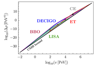
The resulting stochastic gravitational wave background is presented in Fig. 1 for four values of the symmetry breaking scale, in the range of frequencies relevant for the upcoming gravitational wave experiments, whose sensitivities are denoted by the colored regions. If $v\gtrsim 10^{4}\ {\rm PeV}$, the signal can be seen by all the detectors: LISA Amaro-Seoane et al. (2017), DECIGO Kawamura et al. (2011), Big Bang Observer Crowder and Cornish (2005), Einstein Telescope Punturo et al. (2010), and Cosmic Explorer Reitze et al. (2019). This is illustrated in more detail in Fig. 2, which shows the reach of each experiment in terms of the symmetry breaking scale leading to a cosmic string signal. The lower bound is detector-specific, whereas the upper bound reflects the cosmic microwave background constraint in Eq. (20).

The cosmic string network will be produced if either ${\rm U}(1)_{B}$ or ${\rm U}(1)_{L}$ is spontaneously broken by a single scalar. Therefore, among the cases enumerated in Section II, the gravitational wave signals discussed here are relevant in case $(a)$ for both baryon and lepton number breaking, in case $(b)$ only for lepton number breaking, and in case $(c)$ only for baryon number breaking.

The profile of the domain wall configuration $\vec{\phi}_{dw}(z)$ is the solution to the equation Chen et al. (2020)

$\displaystyle\frac{d^{2}\vec{\phi}_{dw}(z)}{dz^{2}}-\vec{\nabla}_{\!\phi}V_{\rm eff}\big{[}\vec{\phi}_{dw}(z)\big{]}=0\ ,$

(28)

where the $z$-axis was chosen to be perpendicular to the domain wall, and the boundary conditions are,

$\displaystyle\vec{\phi}_{dw}(-\infty)=\vec{\phi}_{\rm vac1}\ ,\ \ \ \ \ \vec{\phi}_{dw}(\infty)=\vec{\phi}_{\rm vac2}.$

(29)

As mentioned earlier, there are only two parameters which describe the gravitational wave spectrum from domain walls. The first of them is the domain wall tension $\sigma$ given by

$\displaystyle\sigma=\int_{-\infty}^{\infty}dz\!\left[\frac{1}{2}\bigg{(}\frac{d\vec{\phi}_{dw}(z)}{dz}\bigg{)}^{2}+V_{\rm eff}\big{[}\vec{\phi}_{dw}(z)\big{]}\right].$

(30)

In the model we are considering, to a good approximation

$\displaystyle\sigma\,\sim\,v^{3}\ .$

(31)

The other parameter is the potential bias $\Delta\rho$, i.e., the energy density difference between the vacua, in our case equal to

$\displaystyle\Delta\rho=\big{(}m_{12}^{2}+\tfrac{1}{2}\lambda_{4}v_{1}^{2}+\tfrac{1}{2}\lambda_{5}v_{2}^{2}\big{)}\,v_{1}v_{2}\ .$

(32)

The created domain walls are unstable and undergo annihilation, emitting gravitational radiation, provided that Saikawa (2017)

$\displaystyle\Delta\rho\gtrsim\left(\frac{\sigma}{M_{Pl}}\right)^{2}\ .$

(33)

If in Eq. (32) the term involving $m_{12}^{2}$ is the dominant one, then Eq. (33) takes the form $m_{12}\gtrsim{v^{2}}/{M_{Pl}}$. For example, if the symmetry breaking scale is $v\sim 10^{3}\ \rm PeV$, this implies $m_{12}\gtrsim 100\ {\rm MeV}$. An independent constraint arises from the necessity of domain wall annihilation happening before Big Bang nucleosynthesis, so the ratios of the produced elements are not altered, but the bound in Eq. (33) remains stronger.

Domain wall annihilation leads to a stochastic gravitational wave background given by Kadota et al. (2015); Saikawa (2017),

	$\displaystyle h^{2}\Omega_{\rm DW}(f)$	$\displaystyle\approx$	$\displaystyle 7.1\times 10^{-33}\left(\frac{\sigma}{\rm PeV^{3}}\right)^{4}\left(\frac{\rm TeV^{4}}{\Delta\rho}\right)^{2}\left(\frac{100}{g_{*}}\right)^{\frac{1}{3}}$		(34)
		$\displaystyle\times$	$\displaystyle\!\!\bigg{[}\!\left(\frac{f}{f_{d}}\right)^{3}\!\theta(f_{d}-f)+\left(\frac{f_{d}}{f}\right)\theta(f-f_{d})\bigg{]},\ \ \ \ \ \ \$

where for the area parameter we used $\mathcal{A}=0.8$ and for the efficiency parameter we adopted the value $\tilde{\epsilon}_{\rm gw}=0.7$ Hiramatsu et al. (2014),$\theta$ denotes the step function, and the peak frequency $f_{d}$ is

$\displaystyle f_{d}\approx(0.14\ {\rm Hz})\,\sqrt{\frac{\rm PeV^{3}}{\sigma}\frac{\Delta\rho}{\rm TeV^{4}}}\ .$

(35)

The slope of the signal falls $\sim f^{3}$ to the left of the peak when moving toward lower frequencies, and falls like $f^{-1}$ to the right of the peak when moving toward higher frequencies. The cosmic microwave background constraint on the strength of the signal at the peak is $h^{2}\Omega(f)<2.9\times 10^{-7}$ Clarke et al. (2020), which translates to the following condition on the parameters,

$\displaystyle\frac{\sigma}{\sqrt{\Delta\rho}}\lesssim 2.5\times 10^{12}\ \rm PeV\ ,$

(36)

stronger than the bound imposed by Eq. (33).

Several examples of gravitational wave spectra from domain wall annihilation, plotted using Eq. (34), are shown in Fig. 3 for representative values of the parameters $v$ and $\Delta\rho$. The reach of the upcoming gravitational wave detectors is also shown, including LISA, Big Bang Observer, DECIGO, Einstein Telescope, and Cosmic Explorer. A more detailed look at their sensitivity is provided by Fig. 4, which shows the full parameter space that can be probed by those experiments. The lower bound on the domain wall parameter $\Delta\rho$ is a reflection of the cosmic microwave background constraint from Eq. (36). The parameter $\Delta\rho$ depends in general on all three fundamental Lagrangian parameters $m_{12}$, $\lambda_{4}$, and $\lambda_{5}$ through the relation in Eq. (32). Under the assumption that the term involving $m_{12}$ is dominant, the experimental sensitivity plot in the plane $(v,m_{12})$ would be the same as in figure 4 of Fornal et al. (2023).

The effective potential for the background field $\phi$ consists of the tree-level part, the one-loop Coleman-Weinberg zero temperature correction, and the finite temperature contribution. Upon imposing the condition that the minimum of the zero temperature potential and the mass of $\phi$ remain at their tree-level values (i.e., the cutoff regularization scheme), the effective potential is given by

	$\displaystyle V_{\rm eff}(\phi,T)=-\frac{1}{2}\lambda v^{2}\phi^{2}+\frac{1}{4}\lambda\phi^{4}$
	$\displaystyle+\sum_{i}\frac{n_{i}m_{i}^{2}(\phi)}{64\pi^{2}}\bigg{\{}\!m_{i}^{2}(\phi)\!\left[\log\!\left(\frac{m_{i}^{2}(\phi)}{m_{i}^{2}(v)}\right)\!-\!\frac{3}{2}\right]\!+\!2m_{i}^{2}(v)\!\bigg{\}}$
	$\displaystyle+\ \frac{T^{4}}{2\pi^{2}}\sum_{i}n_{i}\int_{0}^{\infty}dx\,x^{2}\log\left(1\mp e^{-\sqrt{{m_{i}^{2}(\phi)}/{T^{2}}+x^{2}}}\right)$
	$\displaystyle+\ \frac{T}{12\pi}\sum_{j}n^{\prime}_{j}\left\{m_{j}^{3}(\phi)-\left[m_{j}^{2}(\phi)+\Pi_{j}(T)\right]^{\frac{3}{2}}\right\}\ .$		(37)

In the expression above the sums are over all particles charged under the ${\rm U}(1)$ including the Goldstone bosons $\chi_{\rm GB}$, $m_{i}(\phi)$ are the field-dependent masses, $n_{i}$ is the number of degrees of freedom for a given particle ($n_{Z^{\prime}}=3$, $n_{\phi}=1$, $n_{\chi_{\rm GB}}=1$), $n_{j}^{\prime}$ is similar but includes only scalars and longitudinal components of vector bosons ($n^{\prime}_{Z^{\prime}}=1$, $n^{\prime}_{\phi}=1$, $n^{\prime}_{\chi_{\rm GB}}=1$), and for the Goldstones one needs to replace $m_{\chi_{\rm GB}}(v)\to m_{\phi}(v)$. We will assume that all new Yukawa couplings are small, so that the only relevant field-dependent masses are

	$\displaystyle m_{Z^{\prime}}(\phi)=xg\phi\ ,\ \ \ \ m_{\phi}(\phi)=\sqrt{\lambda(3\phi^{2}-v^{2})}\ ,$
	$\displaystyle m_{\chi_{\rm GB}}(\phi)=\sqrt{\lambda(\phi^{2}-v^{2})}\ .$		(38)

In the limit $\lambda\ll g$, the thermal masses are

	$\displaystyle\Pi_{Z^{\prime}}(T)$	$\displaystyle=$	$\displaystyle\frac{1}{3}\left(x^{2}+\frac{9}{2}\right)g^{2}T^{2}\ ,$
	$\displaystyle\Pi_{\phi}(T)$	$\displaystyle=$	$\displaystyle\Pi_{\chi_{\rm GB}}(T)=\frac{1}{4}x^{2}g^{2}T^{2}\ ,$		(39)

where for gauged baryon number $g=g_{B}$ and $x=3$, while for gauged lepton number $g=g_{L}$ and $x=2$.

For a range of $\lambda$ and $g$ values the effective potential develops a vacuum at $\phi\neq 0$ (true vacuum) with a lower energy density than the high temperature vacuum at $\phi=0$ (false vacuum), separated by a potential bump, which are precisely the conditions needed for a first order phase transition to take place. The changing shape of the effective potential is shown in Fig. 5 for a particular choice of parameters, in the case of gauged baryon number.

A first order phase transition from the false vacuum to the true vacuum of a given patch of the Universe corresponds to the nucleation of a bubble which then starts expanding. This process is initiated at the nucleation temperature $T_{*}$, which is determined from the condition that the bubble nucleation rate Linde (1983) becomes comparable with the Hubble expansion,

$\displaystyle\bigg{(}\frac{S(T_{*})}{2\pi T_{*}}\bigg{)}^{3/2}T_{*}^{4}\,e^{-{S(T_{*})}/{T_{*}}}\approx H(T_{*})^{4}\ ,$

(40)

where $S(T)$ is the Euclidean action given by

$\displaystyle S(T)=\int d^{3}r\left[\frac{1}{2}\left(\frac{d\phi_{b}}{dr}\right)^{2}+V_{\rm eff}(\phi_{b},T)\right],$

(41)

with $\phi_{b}$ being the solution of the bubble equation,

$\displaystyle\frac{d^{2}\phi}{dr^{2}}+\frac{2}{r}\frac{d\phi}{dr}-\frac{dV_{\rm eff}(\phi,T)}{d\phi}=0\ ,$

(42)

subject to the boundary conditions

$\displaystyle\frac{d\phi}{dr}\bigg{|}_{r=0}=0\ ,\ \ \ \ \ \phi(\infty)=\phi_{\rm false}\ .$

(43)

Since $H(T)\approx(T^{2}/M_{Pl})\sqrt{4\pi^{3}g_{*}/45}$, Eq. (40) becomes

$\displaystyle\frac{S(T_{*})}{T_{*}}\approx 4\log\!\left(\frac{M_{Pl}}{T_{*}}\right)\!-\!\log\left[\left(\frac{4\pi^{3}g_{*}}{45}\right)^{\!\!2}\!\left(\frac{2\pi\,T_{*}}{S(T_{*})}\right)^{\!\!\frac{3}{2}}\right]\!.\ \$

(44)

The phase transition parameters relevant for determining the gravitational wave signal are: the bubble wall velocity $v_{w}$, the nucleation temperature $T_{*}$, the phase transition strength $\alpha$, and its duration $1/\tilde{\beta}$. In our analysis we assume $v_{w}=c$, but other choices are also possible Espinosa et al. (2010); Caprini et al. (2016). The other three parameters, $T_{*}$, $\alpha$, and $\tilde{\beta}$, are determined from the behavior of the effective potential with changing temperature. As such, those parameters encode information about the details of the particle physics model considered.

The phase transition strength is calculated as the ratio of the energy density difference between the false and true vacuum, and that of radiation, both taken at nucleation temperature,

$\displaystyle\alpha=\frac{\rho_{\rm vac}(T_{*})}{\rho_{\rm rad}(T_{*})}\ .$

(45)

Those two quantities are obtained from the relations

	$\displaystyle\rho_{\rm vac}(T)$	$\displaystyle=$	$\displaystyle V_{\rm eff}(\phi_{\rm false},T)-V_{\rm eff}(\phi_{\rm true},T)$
		$\displaystyle-$	$\displaystyle T\frac{\partial}{\partial T}{\left[V_{\rm eff}(\phi_{\rm false},T)-V_{\rm eff}(\phi_{\rm true},T)\right]}\ ,$
	$\displaystyle\rho_{\rm rad}(T)$	$\displaystyle=$	$\displaystyle\frac{\pi^{2}}{30}g_{*}T^{4}\ ,$		(46)

where $g_{*}$ is the number of degrees of freedom active when the bubbles are nucleated. The parameter $\tilde{\beta}$, related to the time scale of the phase transition, is determined via

$\displaystyle\tilde{\beta}=T_{*}\frac{d}{dT}\bigg{(}\frac{S(T)}{T}\bigg{)}\bigg{|}_{T=T_{*}}\ .$

(47)

The dynamics of the nucleated bubbles generates gravitational waves through sound shock waves in the early Universe plasma, bubble collisions, and magnetohydrodynamic turbulence. The expected contribution of each of those processes to the stochastic gravitational wave background was determined through numerical simulations, and the corresponding empirical formulas were derived. The resulting gravitational wave signal is the sum of the three contributions,

$\displaystyle h^{2}\Omega_{\rm PT}(f)=h^{2}\Omega_{s}(f)+h^{2}\Omega_{c}(f)+h^{2}\Omega_{t}(f)\ .$

(48)

The expected signal from sound waves is Hindmarsh et al. (2014); Caprini et al. (2016)

	$\displaystyle h^{2}\Omega_{s}(f)\,$	$\displaystyle\approx$	$\displaystyle\,\frac{1.9\times 10^{-5}}{\tilde{\beta}}\left(\frac{\kappa_{s}\,\alpha}{\alpha+1}\right)^{2}\left(\frac{100}{g_{*}}\right)^{\frac{1}{3}}\Upsilon$		(49)
		$\displaystyle\times$	$\displaystyle\frac{(f/f_{s})^{3}}{\big{[}1+0.75(f/f_{s})^{2}\big{]}^{7/2}}\ ,$

where $f_{s}$ is the peak frequency, $\kappa_{s}$ is the fraction of the latent heat transformed into the bulk motion of the plasma Espinosa et al. (2010), and $\Upsilon$ is the suppression factor Ellis et al. (2020b); Guo et al. (2021),

	$\displaystyle f_{s}$	$\displaystyle=$	$\displaystyle(0.19\ {\rm Hz})\left(\frac{T_{*}}{1\ {\rm PeV}}\right)\left(\frac{g_{*}}{100}\right)^{\frac{1}{6}}\tilde{\beta}\ ,$
	$\displaystyle\kappa_{s}$	$\displaystyle=$	$\displaystyle\frac{\alpha}{0.73+0.083\sqrt{\alpha}+\alpha}\ ,$
	$\displaystyle\Upsilon\,$	$\displaystyle=$	$\displaystyle 1-\frac{1}{\Big{[}1+\frac{8\pi^{\frac{1}{3}}}{\tilde{\beta}}\big{(}\frac{{\alpha+1}}{3\kappa_{s}\alpha}\big{)}^{\frac{1}{2}}\Big{]}^{\frac{1}{2}}}\ .$		(50)

The signal from bubble wall collisions is Kosowsky et al. (1992); Huber and Konstandin (2008); Caprini et al. (2016) (see Lewicki and Vaskonen (2021) for recent updates)

	$\displaystyle h^{2}\Omega_{c}(f)\,$	$\displaystyle\approx$	$\displaystyle\,\frac{4.9\times 10^{-6}}{\tilde{\beta}^{2}}\left(\frac{\kappa_{c}\,\alpha}{\alpha+1}\right)^{2}\left(\frac{100}{g_{*}}\right)^{\frac{1}{3}}$		(51)
		$\displaystyle\times$	$\displaystyle\frac{(f/f_{c})^{2.8}}{1+2.8(f/f_{c})^{3.8}}\ ,\ \ \ \ \ \$

where now $f_{c}$ is the peak frequency and $\kappa_{c}$ is the fraction of the latent heat deposited into the bubble front Kamionkowski et al. (1994),

	$\displaystyle f_{c}$	$\displaystyle=$	$\displaystyle(0.037\ {\rm Hz})\left(\frac{T_{*}}{1\ {\rm PeV}}\right)\left(\frac{g_{*}}{100}\right)^{\frac{1}{6}}\tilde{\beta}\ ,$
	$\displaystyle\kappa_{c}$	$\displaystyle=$	$\displaystyle\frac{\frac{4}{27}\sqrt{\frac{3}{2}\alpha}+0.72\,\alpha}{1+0.72\,\alpha}\ .$		(52)

The final contribution is provided by turbulence Caprini and Durrer (2006); Caprini et al. (2009),

	$\displaystyle h^{2}\Omega_{t}(f)\,$	$\displaystyle\approx$	$\displaystyle\,\frac{3.4\times 10^{-4}}{\tilde{\beta}}\left(\frac{\epsilon\,\kappa_{s}\,\alpha}{\alpha+1}\right)^{\frac{3}{2}}\left(\frac{100}{g_{*}}\right)^{\frac{1}{3}}$		(53)
		$\displaystyle\times$	$\displaystyle\frac{({f}/{f_{t}})^{3}}{\big{(}1+{8\pi f}/{f_{*}}\big{)}\big{(}1+{f}/{f_{t}}\big{)}^{{11}/{3}}}\ ,$

where $\epsilon=0.05$ Caprini et al. (2016), while the peak frequency $f_{t}$ and the parameter $f_{*}$ are

	$\displaystyle f_{t}$	$\displaystyle=$	$\displaystyle(0.27\ {\rm Hz})\left(\frac{g_{*}}{100}\right)^{\frac{1}{6}}\left(\frac{T_{*}}{1\ {\rm PeV}}\right)\tilde{\beta}\ ,$
	$\displaystyle f_{*}$	$\displaystyle=$	$\displaystyle(0.17\ {\rm Hz})\left(\frac{g_{*}}{100}\right)^{\frac{1}{6}}\left(\frac{T_{*}}{1\ {\rm PeV}}\right)\ .$		(54)

The resulting gravitational wave signals from the first order phase transition triggered by ${\rm U}(1)_{B}$ breaking are shown in Fig. 6 for several symmetry breaking scales: $10\ {\rm TeV}$ (light brown curve), $100\ {\rm TeV}$ (brown curve), $1\ {\rm PeV}$ (purple curve), and $10\ {\rm PeV}$ (black curve). The gauge coupling was assumed to be $g_{B}=0.25$, and the quartic coupling was chosen to be $\lambda_{B}=0.006$. Spectra with peaks at larger frequencies correspond to higher symmetry breaking scales.

The effect of the suppression factor $\Upsilon$ reducing the sound wave contribution in Eq. (49) is that the bubble collision and turbulence components become distinguishable in the spectrum. Although the main peak is still due to sound waves, the slope at lower frequencies is dominated by bubble collisions, whereas for higher frequencies the turbulence contribution visibly changes the slope of the curve. Without the suppression factor, the spectrum would be determined, to a good approximation, just by the sound wave component in the region relevant for future detectors.

Depending on the Lagrangian parameters, the signal may be detectable in upcoming gravitational wave experiments: LISA, DECIGO, Big Bang Observer, Einstein Telescope, and Cosmic Explorer. To study this more quantitatively, in Fig. 7 we show part of the $(g_{B},\lambda_{B})$ parameter space for which the signal can be detected in each experiment when $v_{B}=1\ {\rm PeV}$. Specifically, the upper boundary for each detector corresponds to a signal-to-noise ratio of five upon a single year of data taking, while the lower boundary arises when either $S(T)/T$ is too large to satisfy Eq. (44) or the new vacuum has an energy density larger than that of the high temperature vacuum.

As mentioned earlier, our analysis of the first order phase transition signal from ${\rm U}(1)_{B}$ breaking differs from the one in Fornal and Shams Es Haghi (2020) in several aspects. The fermionic particle content in Eq. (II) is different, and we chose the corresponding Yukawa couplings to be small, which is a more minimal scenario than $Y=0.6$ in Fornal and Shams Es Haghi (2020). Our analysis is also applicable to ${\rm U}(1)_{L}$ breaking, since we calculate the thermal masses in the general case – this result will be used in Section VII. Finally, when determining the gravitational wave signal we included the effect of bubble collisions, which was not considered in Fornal and Shams Es Haghi (2020), but which increases the reach of upcoming detectors due to the enhancement of the signal in the lower frequency region.

A new gravitational wave signature arises when each of the two ${\rm U}(1)$ symmetries is broken by two scalars, leading to the production of domain walls at two different energy scales during the evolution of the Universe. The signal consists of two sharp domain wall peaks. The slope on the left side of each peak depends on the frequency like $\sim f^{3}$, whereas the slope on the right side of the peak falls like $\sim 1/f$. There is a nontrivial structure created between the two peaks, which can be used to distinguish this type of signal from others. If the two symmetry breaking scales are high, this signature can be searched for in all the upcoming gravitational wave experiments we considered: LISA, DECIGO, Big Bang Observer, Einstein Telescope, and Cosmic Explorer. A realization of this scenario in our model is shown in Fig. 8, where the parameters for the ${\rm U(1)}_{B}$ breaking were chosen to be $v_{B}=10^{3}\ {\rm PeV}$ and $\Delta\rho=10^{-5}\ {\rm PeV^{4}}$, whereas for the ${\rm U(1)}_{L}$ breaking they are $v_{L}=5\times 10^{4}\ {\rm PeV}$ and $\Delta\rho=1.6\times 10^{5}\ {\rm PeV^{4}}$.

Another gravitational wave signature, not considered in the literature before, is realized when one of the ${\rm U}(1)$ symmetries is broken by one scalar, leading to cosmic string production, whereas the other ${\rm U}(1)$ is broken by two scalars, resulting in domain wall creation. If the two symmetry breaking scales are high, their contributions may overlap and produce a very unusual domain wall peak over the cosmic string background. An example is shown in Fig. 9, where the symmetry breaking scale for ${\rm U}(1)_{L}$ was chosen to be $v_{L}=10^{6}\ {\rm PeV}$, whereas the parameters for ${\rm U}(1)_{B}$ breaking are $v_{B}=8\times 10^{3}\ {\rm PeV}$ and $\Delta\rho=2\ {\rm PeV^{4}}$. For this particular selection of parameters, Big Bang Observer and DECIGO can probe the peak area, but for lower ${\rm U}(1)_{B}$ breaking scales this structure is accessible to LISA, whereas higher symmetry breaking scales would make it detectable by Einstein Telescope and Cosmic Explorer.

References

- Glashow (1961) S. L. Glashow, Partial Symmetries of Weak Interactions, Nucl. Phys. 22, 579–588 (1961).
- Higgs (1964) P. W. Higgs, Broken Symmetries and the Masses of Gauge Bosons, Phys. Rev. Lett. 13, 508–509 (1964).
- Englert and Brout (1964) F. Englert and R. Brout, Broken Symmetry and the Mass of Gauge Vector Mesons, Phys. Rev. Lett. 13, 321–323 (1964).
- Weinberg (1967) S. Weinberg, A Model of Leptons, Phys. Rev. Lett. 19, 1264–1266 (1967).
- Salam (1968) A. Salam, Weak and Electromagnetic Interactions, 8th Nobel Symposium Lerum, Sweden, May 19-25, 1968, Conf. Proc. C 680519, 367–377 (1968).
- Fritzsch et al. (1973) H. Fritzsch, M. Gell-Mann, and H. Leutwyler, Advantages of the Color Octet Gluon Picture, Phys. Lett. B 47, 365–368 (1973).
- Gross and Wilczek (1973) D. J. Gross and F. Wilczek, Ultraviolet Behavior of Nonabelian Gauge Theories, Phys. Rev. Lett. 30, 1343–1346 (1973).
- Politzer (1973) H. D. Politzer, Reliable Perturbative Results for Strong Interactions? Phys. Rev. Lett. 30, 1346–1349 (1973).
- Georgi and Glashow (1974) H. Georgi and S. L. Glashow, Unity of All Elementary Particle Forces, Phys. Rev. Lett. 32, 438–441 (1974).
- Fritzsch and Minkowski (1975) H. Fritzsch and P. Minkowski, Unified Interactions of Leptons and Hadrons, Annals Phys. 93, 193–266 (1975).
- Abe et al. (2017) K. Abe et al. (Super-Kamiokande), Search for Proton Decay via and in 0.31 Megaton·Years Exposure of the Super-Kamiokande Water Cherenkov Detector, Phys. Rev. D 95, 012004 (2017), arXiv:1610.03597 [hep-ex] .
- Kallosh et al. (1995) R. Kallosh, A. D. Linde, D. A. Linde, and L. Susskind, Gravity and Global Symmetries, Phys. Rev. D 52, 912–935 (1995), arXiv:hep-th/9502069 .
- Pais (1973) A. Pais, Remark on Baryon Conservation, Phys. Rev. D 8, 1844–1846 (1973).
- Rajpoot (1988) S. Rajpoot, Gauge Symmetries of Electroweak Interactions, Int. J. Theor. Phys. 27, 689 (1988).
- Foot et al. (1989) R. Foot, G. C. Joshi, and H. Lew, Gauged Baryon and Lepton Numbers, Phys. Rev. D 40, 2487–2489 (1989).
- Carone and Murayama (1995) C. D. Carone and H. Murayama, Realistic Models with a Light U(1) Gauge Boson Coupled to Baryon Number, Phys. Rev. D 52, 484–493 (1995), arXiv:hep-ph/9501220 .
- Georgi and Glashow (1996) H. Georgi and S. L. Glashow, Decays of a Leptophobic Gauge Boson, Phys. Lett. B 387, 341–345 (1996), arXiv:hep-ph/9607202 .
- Fileviez Perez and Wise (2010) P. Fileviez Perez and M. B. Wise, Baryon and Lepton Number as Local Gauge Symmetries, Phys. Rev. D 82, 011901 (2010), [Erratum: Phys.Rev.D 82, 079901 (2010)], arXiv:1002.1754 [hep-ph] .
- Duerr et al. (2013) M. Duerr, P. Fileviez Perez, and M. B. Wise, Gauge Theory for Baryon and Lepton Numbers with Leptoquarks, Phys. Rev. Lett. 110, 231801 (2013), arXiv:1304.0576 [hep-ph] .
- Fileviez Perez et al. (2014) P. Fileviez Perez, S. Ohmer, and H. H. Patel, Minimal Theory for Lepto-Baryons, Phys. Lett. B 735, 283–287 (2014), arXiv:1403.8029 [hep-ph] .
- Arnold et al. (2013) J. M. Arnold, P. Fileviez Perez, B. Fornal, and S. Spinner, B and L at the Supersymmetry Scale, Dark Matter, and R-Parity Violation, Phys. Rev. D 88, 115009 (2013), arXiv:1310.7052 [hep-ph] .
- Fornal et al. (2015) B. Fornal, A. Rajaraman, and T. M. P. Tait, Baryon Number as the Fourth Color, Phys. Rev. D 92, 055022 (2015), arXiv:1506.06131 [hep-ph] .
- Fornal and Tait (2016) B. Fornal and T. M. P. Tait, Dark Matter from Unification of Color and Baryon Number, Phys. Rev. D 93, 075010 (2016), arXiv:1511.07380 [hep-ph] .
- Fornal et al. (2017) B. Fornal, Y. Shirman, T. M. P. Tait, and J. Rittenhouse West, Asymmetric Dark Matter and Baryogenesis from , Phys. Rev. D 96, 035001 (2017), arXiv:1703.00199 [hep-ph] .
- Duerr and Fileviez Perez (2015) M. Duerr and P. Fileviez Perez, Theory for Baryon Number and Dark Matter at the LHC, Phys. Rev. D 91, 095001 (2015), arXiv:1409.8165 [hep-ph] .
- Ohmer and Patel (2015) S. Ohmer and H. H. Patel, Leptobaryons as Majorana Dark Matter, Phys. Rev. D 92, 055020 (2015), arXiv:1506.00954 [hep-ph] .
- Fileviez Perez et al. (2019) P. Fileviez Perez, E. Golias, R.-H. Li, and C. Murgui, Leptophobic Dark Matter and the Baryon Number Violation Scale, Phys. Rev. D 99, 035009 (2019), arXiv:1810.06646 [hep-ph] .
- Fileviez Perez et al. (2021) P. Fileviez Perez, C. Murgui, and A. D. Plascencia, Baryogenesis via Leptogenesis: Spontaneous B and L Violation, Phys. Rev. D 104, 055007 (2021), arXiv:2103.13397 [hep-ph] .
- Abbott et al. (2016) B. P. Abbott et al. (LIGO Scientific, Virgo), Observation of Gravitational Waves from a Binary Black Hole Merger, Phys. Rev. Lett. 116, 061102 (2016), arXiv:1602.03837 [gr-qc] .
- Turner (1997) M. S. Turner, Detectability of Inflation Produced Gravitational Waves, Phys. Rev. D 55, R435–R439 (1997), arXiv:astro-ph/9607066 .
- Kosowsky et al. (1992) A. Kosowsky, M. S. Turner, and R. Watkins, Gravitational Radiation from Colliding Vacuum Bubbles, Phys. Rev. D 45, 4514–4535 (1992).
- Hiramatsu et al. (2010) T. Hiramatsu, M. Kawasaki, and K. Saikawa, Gravitational Waves from Collapsing Domain Walls, JCAP 05, 032 (2010), arXiv:1002.1555 [astro-ph.CO] .
- Vachaspati and Vilenkin (1985a) T. Vachaspati and A. Vilenkin, Gravitational Radiation from Cosmic Strings, Phys. Rev. D 31, 3052 (1985a).
- Sakellariadou (1990) M. Sakellariadou, Gravitational Waves Emitted from Infinite Strings, Phys. Rev. D 42, 354–360 (1990), [Erratum: Phys. Rev. D 43, 4150 (1991)].
- Amaro-Seoane et al. (2017) P. Amaro-Seoane et al. (LISA), Laser Interferometer Space Antenna, (2017), arXiv:1702.00786 [astro-ph.IM] .
- Reitze et al. (2019) D. Reitze et al., Cosmic Explorer: The U.S. Contribution to Gravitational-Wave Astronomy beyond LIGO, Bull. Am. Astron. Soc. 51, 035 (2019), arXiv:1907.04833 [astro-ph.IM] .
- Punturo et al. (2010) M. Punturo et al., The Einstein Telescope: A Third-Generation Gravitational Wave Observatory, Class. Quant. Grav. 27, 194002 (2010).
- Kawamura et al. (2011) S. Kawamura et al., The Japanese Space Gravitational Wave Antenna: DECIGO, Class. Quant. Grav. 28, 094011 (2011).
- Crowder and Cornish (2005) J. Crowder and N. J. Cornish, Beyond LISA: Exploring Future Gravitational Wave Missions, Phys. Rev. D 72, 083005 (2005), arXiv:gr-qc/0506015 .
- Kibble (1976) T. W. B. Kibble, Topology of Cosmic Domains and Strings, J. Phys. A 9, 1387–1398 (1976).
- Buchmuller et al. (2019) W. Buchmuller, V. Domcke, H. Murayama, and K. Schmitz, Probing the Scale of Grand Unification with Gravitational Waves, (2019), arXiv:1912.03695 [hep-ph] .
- King et al. (2020) S. F. King, S. Pascoli, J. Turner, and Y.-L. Zhou, Gravitational Waves and Proton Decay: Complementary Windows into GUTs, (2020), arXiv:2005.13549 [hep-ph] .
- Blanco-Pillado and Olum (2017) J. J. Blanco-Pillado and K. D. Olum, Stochastic Gravitational Wave Background from Smoothed Cosmic String Loops, Phys. Rev. D 96, 104046 (2017), arXiv:1709.02693 [astro-ph.CO] .
- Ringeval and Suyama (2017) C. Ringeval and T. Suyama, Stochastic Gravitational Waves from Cosmic String Loops in Scaling, JCAP 12, 027 (2017), arXiv:1709.03845 [astro-ph.CO] .
- Cui et al. (2018) Y. Cui, M. Lewicki, D. E. Morrissey, and J. D. Wells, Cosmic Archaeology with Gravitational Waves from Cosmic Strings, Phys. Rev. D 97, 123505 (2018), arXiv:1711.03104 [hep-ph] .
- Cui et al. (2019) Y. Cui, M. Lewicki, D. E. Morrissey, and J. D. Wells, Probing the Pre-BBN Universe with Gravitational Waves from Cosmic Strings, JHEP 01, 081 (2019), arXiv:1808.08968 [hep-ph] .
- Guedes et al. (2018) G. S. F. Guedes, P. P. Avelino, and L. Sousa, Signature of Inflation in the Stochastic Gravitational Wave Background Generated by Cosmic String Networks, Phys. Rev. D 98, 123505 (2018), arXiv:1809.10802 [astro-ph.CO] .
- Dror et al. (2020) J. A. Dror, T. Hiramatsu, K. Kohri, H. Murayama, and G. White, Testing the Seesaw Mechanism and Leptogenesis with Gravitational Waves, Phys. Rev. Lett. 124, 041804 (2020), arXiv:1908.03227 [hep-ph] .
- Zhou and Bian (2020) R. Zhou and L. Bian, Gravitational Waves from Cosmic Strings and First-Order Phase Transition, (2020), arXiv:2006.13872 [hep-ph] .
- Gouttenoire et al. (2020a) Y. Gouttenoire, G. Servant, and P. Simakachorn, BSM with Cosmic Strings: Heavy, up to EeV Mass, Unstable Particles, JCAP 07, 016 (2020a), arXiv:1912.03245 [hep-ph] .
- Fornal and Shams Es Haghi (2020) B. Fornal and B. Shams Es Haghi, Baryon and Lepton Number Violation from Gravitational Waves, Phys. Rev. D 102, 115037 (2020), arXiv:2008.05111 [hep-ph] .
- Gouttenoire et al. (2020b) Y. Gouttenoire, G. Servant, and P. Simakachorn, Beyond the Standard Models with Cosmic Strings, JCAP 07, 032 (2020b), arXiv:1912.02569 [hep-ph] .
- Abbott et al. (2021) R. Abbott et al. (LIGO Scientific, Virgo, KAGRA), Constraints on Cosmic Strings Using Data from the Third Advanced LIGO–Virgo Observing Run, Phys. Rev. Lett. 126, 241102 (2021), arXiv:2101.12248 [gr-qc] .
- Eto et al. (2018a) M. Eto, M. Kurachi, and M. Nitta, Constraints on Two Higgs Doublet Models from Domain Walls, Phys. Lett. B 785, 447–453 (2018a), arXiv:1803.04662 [hep-ph] .
- Eto et al. (2018b) M. Eto, M. Kurachi, and M. Nitta, Non-Abelian Strings and Domain Walls in Two Higgs Doublet Models, JHEP 08, 195 (2018b), arXiv:1805.07015 [hep-ph] .
- Chen et al. (2020) N. Chen, T. Li, Z. Teng, and Y. Wu, Collapsing Domain Walls in the Two-Higgs-Doublet Model and Deep Insights from the EDM, JHEP 10, 081 (2020), arXiv:2006.06913 [hep-ph] .
- Battye et al. (2020) R. A. Battye, A. Pilaftsis, and D. G. Viatic, Domain Wall Constraints on Two-Higgs-Doublet Models with Symmetry, Phys. Rev. D 102, 123536 (2020), arXiv:2010.09840 [hep-ph] .
- Kadota et al. (2015) K. Kadota, M. Kawasaki, and K. Saikawa, Gravitational Waves from Domain Walls in the Next-to-Minimal Supersymmetric Standard Model, JCAP 10, 041 (2015), arXiv:1503.06998 [hep-ph] .
- Craig et al. (2021) N. Craig, I. Garcia Garcia, G. Koszegi, and A. McCune, P Not PQ, JHEP 09, 130 (2021), arXiv:2012.13416 [hep-ph] .
- Blasi et al. (2023) S. Blasi, A. Mariotti, A. Rase, A. Sevrin, and K. Turbang, Friction on ALP Domain Walls and Gravitational Waves, JCAP 04, 008 (2023), arXiv:2210.14246 [hep-ph] .
- Dunsky et al. (2022) D. I. Dunsky, A. Ghoshal, H. Murayama, Y. Sakakihara, and G. White, GUTs, Hybrid Topological Defects, and Gravitational Waves, Phys. Rev. D 106, 075030 (2022), arXiv:2111.08750 [hep-ph] .
- Borah and Dasgupta (2022) D. Borah and A. Dasgupta, Probing Left-Right Symmetry via Gravitational Waves from Domain Walls, Phys. Rev. D 106, 035016 (2022), arXiv:2205.12220 [hep-ph] .
- Fornal et al. (2023) B. Fornal, K. Garcia, and E. Pierre, Testing Unification and Dark Matter with Gravitational Waves, (2023), arXiv:2305.12566 [hep-ph] .
- Barman et al. (2022) B. Barman, D. Borah, A. Dasgupta, and A. Ghoshal, Probing High Scale Dirac Leptogenesis via Gravitational Waves from Domain Walls, Phys. Rev. D 106, 015007 (2022), arXiv:2205.03422 [hep-ph] .
- Saikawa (2017) K. Saikawa, A Review of Gravitational Waves from Cosmic Domain Walls, Universe 3, 40 (2017), arXiv:1703.02576 [hep-ph] .
- Jiang and Huang (2022) Y. Jiang and Q.-G. Huang, Implications for Cosmic Domain Walls from the First Three Observing Runs of LIGO-Virgo, Phys. Rev. D 106, 103036 (2022), arXiv:2208.00697 [astro-ph.CO] .
- Grojean and Servant (2007) C. Grojean and G. Servant, Gravitational Waves from Phase Transitions at the Electroweak Scale and Beyond, Phys. Rev. D 75, 043507 (2007), arXiv:hep-ph/0607107 .
- Vaskonen (2017) V. Vaskonen, Electroweak Baryogenesis and Gravitational Waves from a Real Scalar Singlet, Phys. Rev. D 95, 123515 (2017), arXiv:1611.02073 [hep-ph] .
- Dorsch et al. (2017) G. C. Dorsch, S. J. Huber, T. Konstandin, and J. M. No, A Second Higgs Doublet in the Early Universe: Baryogenesis and Gravitational Waves, JCAP 05, 052 (2017), arXiv:1611.05874 [hep-ph] .
- Bernon et al. (2018) J. Bernon, L. Bian, and Y. Jiang, A New Insight into the Phase Transition in the Early Universe with Two Higgs Doublets, JHEP 05, 151 (2018), arXiv:1712.08430 [hep-ph] .
- Chala et al. (2018) M. Chala, C. Krause, and G. Nardini, Signals of the Electroweak Phase Transition at Colliders and Gravitational Wave Observatories, JHEP 07, 062 (2018), arXiv:1802.02168 [hep-ph] .
- Angelescu and Huang (2019) A. Angelescu and P. Huang, Multistep Strongly First Order Phase Transitions from New Fermions at the TeV Scale, Phys. Rev. D 99, 055023 (2019), arXiv:1812.08293 [hep-ph] .
- Alves et al. (2019) A. Alves, T. Ghosh, H.-K. Guo, K. Sinha, and D. Vagie, Collider and Gravitational Wave Complementarity in Exploring the Singlet Extension of the Standard Model, JHEP 04, 052 (2019), arXiv:1812.09333 [hep-ph] .
- Han et al. (2021) X.-F. Han, L. Wang, and Y. Zhang, Dark Matter, Electroweak Phase Transition, and Gravitational Waves in the Type II Two-Higgs-Doublet Model with a Singlet Scalar Field, Phys. Rev. D 103, 035012 (2021), arXiv:2010.03730 [hep-ph] .
- Benincasa et al. (2022) N. Benincasa, L. Delle Rose, K. Kannike, and L. Marzola, Multistep Phase Transitions and Gravitational Waves in the Inert Doublet Model, (2022), arXiv:2205.06669 [hep-ph] .
- Craig et al. (2020) N. Craig, N. Levi, A. Mariotti, and D. Redigolo, Ripples in Spacetime from Broken Supersymmetry, JHEP 21, 184 (2020), arXiv:2011.13949 [hep-ph] .
- Fornal et al. (2021) B. Fornal, B. Shams Es Haghi, J.-H. Yu, and Y. Zhao, Gravitational Waves from Mini-Split SUSY, Phys. Rev. D 104, 115005 (2021), arXiv:2104.00747 [hep-ph] .
- Dev et al. (2019) P. S. B. Dev, F. Ferrer, Y. Zhang, and Y. Zhang, Gravitational Waves from First-Order Phase Transition in a Simple Axion-Like Particle Model, JCAP 11, 006 (2019), arXiv:1905.00891 [hep-ph] .
- Von Harling et al. (2020) B. Von Harling, A. Pomarol, O. Pujolas, and F. Rompineve, Peccei-Quinn Phase Transition at LIGO, JHEP 04, 195 (2020), arXiv:1912.07587 [hep-ph] .
- Delle Rose et al. (2020) L. Delle Rose, G. Panico, M. Redi, and A. Tesi, Gravitational Waves from Supercool Axions, JHEP 04, 025 (2020), arXiv:1912.06139 [hep-ph] .
- Croon et al. (2019) D. Croon, T. E. Gonzalo, and G. White, Gravitational Waves from a Pati-Salam Phase Transition, JHEP 02, 083 (2019), arXiv:1812.02747 [hep-ph] .
- Huang et al. (2020) W.-C. Huang, F. Sannino, and Z.-W. Wang, Gravitational Waves from Pati-Salam Dynamics, Phys. Rev. D 102, 095025 (2020), arXiv:2004.02332 [hep-ph] .
- Okada et al. (2021) N. Okada, O. Seto, and H. Uchida, Gravitational Waves from Breaking of an Extra in Grand Unification, PTEP 2021, 033B01 (2021), arXiv:2006.01406 [hep-ph] .
- Hasegawa et al. (2019) T. Hasegawa, N. Okada, and O. Seto, Gravitational Waves from the Minimal Gauged Model, Phys. Rev. D 99, 095039 (2019), arXiv:1904.03020 [hep-ph] .
- Brdar et al. (2019) V. Brdar, A. J. Helmboldt, and J. Kubo, Gravitational Waves from First-Order Phase Transitions: LIGO as a Window to Unexplored Seesaw Scales, JCAP 02, 021 (2019), arXiv:1810.12306 [hep-ph] .
- Okada and Seto (2018) N. Okada and O. Seto, Probing the Seesaw Scale with Gravitational Waves, Phys. Rev. D 98, 063532 (2018), arXiv:1807.00336 [hep-ph] .
- Di Bari et al. (2021) P. Di Bari, D. Marfatia, and Y.-L. Zhou, Gravitational Waves from First-Order Phase Transitions in Majoron Models of Neutrino Mass, JHEP 10, 193 (2021), arXiv:2106.00025 [hep-ph] .
- Zhou et al. (2022) R. Zhou, L. Bian, and Y. Du, Electroweak Phase Transition and Gravitational Waves in the Type-II Seesaw Model, JHEP 08, 205 (2022), arXiv:2203.01561 [hep-ph] .
- Greljo et al. (2020) A. Greljo, T. Opferkuch, and B. A. Stefanek, Gravitational Imprints of Flavor Hierarchies, Phys. Rev. Lett. 124, 171802 (2020), arXiv:1910.02014 [hep-ph] .
- Fornal (2021) B. Fornal, Gravitational Wave Signatures of Lepton Universality Violation, Phys. Rev. D 103, 015018 (2021), arXiv:2006.08802 [hep-ph] .
- Schwaller (2015) P. Schwaller, Gravitational Waves from a Dark Phase Transition, Phys. Rev. Lett. 115, 181101 (2015), arXiv:1504.07263 [hep-ph] .
- Breitbach et al. (2019) M. Breitbach, J. Kopp, E. Madge, T. Opferkuch, and P. Schwaller, Dark, Cold, and Noisy: Constraining Secluded Hidden Sectors with Gravitational Waves, JCAP 07, 007 (2019), arXiv:1811.11175 [hep-ph] .
- Croon et al. (2018) D. Croon, V. Sanz, and G. White, Model Discrimination in Gravitational Wave spectra from Dark Phase Transitions, JHEP 08, 203 (2018), arXiv:1806.02332 [hep-ph] .
- Hall et al. (2020) E. Hall, T. Konstandin, R. McGehee, H. Murayama, and G. Servant, Baryogenesis From a Dark First-Order Phase Transition, JHEP 04, 042 (2020), arXiv:1910.08068 [hep-ph] .
- Ellis et al. (2020a) J. Ellis, M. Lewicki, and V. Vaskonen, Updated Predictions for Gravitational Waves Produced in a Strongly Supercooled Phase Transition, JCAP 11, 020 (2020a), arXiv:2007.15586 [astro-ph.CO] .
- Kawana (2022) K. Kawana, Cosmology of a Supercooled Universe, Phys. Rev. D 105, 103515 (2022), arXiv:2201.00560 [hep-ph] .
- Baldes (2017) I. Baldes, Gravitational Waves from the Asymmetric-Dark-Matter Generating Phase Transition, JCAP 05, 028 (2017), arXiv:1702.02117 [hep-ph] .
- Azatov et al. (2021) A. Azatov, M. Vanvlasselaer, and W. Yin, Dark Matter Production from Relativistic Bubble Walls, JHEP 03, 288 (2021), arXiv:2101.05721 [hep-ph] .
- Costa et al. (2022a) F. Costa, S. Khan, and J. Kim, A Two-Component Dark Matter Model and its Associated Gravitational Waves, JHEP 06, 026 (2022a), arXiv:2202.13126 [hep-ph] .
- Costa et al. (2022b) F. Costa, S. Khan, and J. Kim, A Two-Component Vector WIMP – Fermion FIMP Dark Matter Model with an Extended Seesaw Mechanism, JHEP 12, 165 (2022b), arXiv:2209.13653 [hep-ph] .
- Fornal and Pierre (2022) B. Fornal and E. Pierre, Asymmetric Dark Matter from Gravitational Waves, Phys. Rev. D 106, 115040 (2022), arXiv:2209.04788 [hep-ph] .
- Kierkla et al. (2023) M. Kierkla, A. Karam, and B. Swiezewska, Conformal Model for Gravitational Waves and Dark Matter: A Status Update, JHEP 03, 007 (2023), arXiv:2210.07075 [astro-ph.CO] .
- Azatov et al. (2022) A. Azatov, G. Barni, S. Chakraborty, M. Vanvlasselaer, and W. Yin, Ultra-Relativistic Bubbles from the Simplest Higgs Portal and their Cosmological Consequences, JHEP 10, 017 (2022), arXiv:2207.02230 [hep-ph] .
- Caldwell et al. (2022) R. Caldwell et al., Detection of Early-Universe Gravitational-Wave Signatures and Fundamental Physics, Gen. Rel. Grav. 54, 156 (2022), arXiv:2203.07972 [gr-qc] .
- Athron et al. (2023) P. Athron, C. Balazs, A. Fowlie, L. Morris, and L. Wu, Cosmological Phase Transitions: From Perturbative Particle Physics to Gravitational Waves, (2023), arXiv:2305.02357 [hep-ph] .
- Badger et al. (2023) C. Badger, B. Fornal, K. Martinovic, A. Romero, K. Turbang, H. Guo, A. Mariotti, M. Sakellariadou, A. Sevrin, F.-W. Yang, and Y. Zhao, Probing Early Universe Supercooled Phase Transitions with Gravitational Wave Data, Phys. Rev. D 107, 023511 (2023), arXiv:2209.14707 [hep-ph] .
- Ellis et al. (2019) J. Ellis, M. Lewicki, J. M. No, and V. Vaskonen, Gravitational Wave Energy Budget in Strongly Supercooled Phase Transitions, JCAP 06, 024 (2019), arXiv:1903.09642 [hep-ph] .
- Lewicki and Vaskonen (2020a) M. Lewicki and V. Vaskonen, On Bubble Collisions in Strongly Supercooled Phase Transitions, Phys. Dark Univ. 30, 100672 (2020a), arXiv:1912.00997 [astro-ph.CO] .
- Lewicki and Vaskonen (2020b) M. Lewicki and V. Vaskonen, Gravitational Wave Spectra from Strongly Supercooled Phase Transitions, Eur. Phys. J. C 80, 1003 (2020b), arXiv:2007.04967 [astro-ph.CO] .
- Aghanim et al. (2020) N. Aghanim et al. (Planck), Planck 2018 Results. VI. Cosmological Parameters, Astron. Astrophys. 641, A6 (2020), [Erratum: Astron.Astrophys. 652, C4 (2021)], arXiv:1807.06209 [astro-ph.CO] .
- Davidson et al. (2008) S. Davidson, E. Nardi, and Y. Nir, Leptogenesis, Phys. Rept. 466, 105–177 (2008), arXiv:0802.2962 [hep-ph] .
- Buchmuller et al. (2005) W. Buchmuller, P. Di Bari, and M. Plumacher, Leptogenesis for Pedestrians, Annals Phys. 315, 305–351 (2005), arXiv:hep-ph/0401240 .
- Workman et al. (2022) R. L. Workman et al. (Particle Data Group), Review of Particle Physics, PTEP 2022, 083C01 (2022).
- Vilenkin and Shellard (2000) A. Vilenkin and E. P. S. Shellard, Cosmic Strings and Other Topological Defects, Cambridge University Press (2000).
- Ade et al. (2014) P. A. R. Ade et al. (Planck), Planck 2013 Results. XXV. Searches for Cosmic Strings and Other Topological Defects, Astron. Astrophys. 571, A25 (2014), arXiv:1303.5085 [astro-ph.CO] .
- Olum and Blanco-Pillado (2000) K. D. Olum and J. J. Blanco-Pillado, Radiation from Cosmic String Standing Waves, Phys. Rev. Lett. 84, 4288–4291 (2000), arXiv:astro-ph/9910354 .
- Moore et al. (2002) J. N. Moore, E. P. S. Shellard, and C. J. A. P. Martins, On the Evolution of Abelian-Higgs String Networks, Phys. Rev. D 65, 023503 (2002), arXiv:hep-ph/0107171 .
- Kibble (1985) T. W. B. Kibble, Evolution of a System of Cosmic Strings, Nucl. Phys. B 252, 227 (1985), [Erratum: Nucl.Phys.B 261, 750 (1985)].
- Bennett and Bouchet (1988) D. P. Bennett and F. R. Bouchet, Evidence for a Scaling Solution in Cosmic-String Evolution, Phys. Rev. Lett. 60, 257–260 (1988).
- Bennett and Bouchet (1989) D. P. Bennett and F. R. Bouchet, Cosmic-String Evolution, Phys. Rev. Lett. 63, 2776–2779 (1989).
- Albrecht and Turok (1989) A. Albrecht and N. Turok, Evolution of Cosmic String Networks, Phys. Rev. D 40, 973–1001 (1989).
- Allen and Shellard (1990) B. Allen and E. P. S. Shellard, Cosmic-String Evolution: A Numerical Simulation, Phys. Rev. Lett. 64, 119–122 (1990).
- Hindmarsh and Kibble (1995) M. B. Hindmarsh and T. W. B. Kibble, Cosmic Strings, Rept. Prog. Phys. 58, 477–562 (1995), arXiv:hep-ph/9411342 .
- Blanco-Pillado et al. (2014) J. J. Blanco-Pillado, K. D. Olum, and B. Shlaer, The Number of Cosmic String Loops, Phys. Rev. D 89, 023512 (2014), arXiv:1309.6637 [astro-ph.CO] .
- Vachaspati and Vilenkin (1985b) T. Vachaspati and A. Vilenkin, Gravitational Radiation from Cosmic Strings, Phys. Rev. D 31, 3052–3058 (1985b).
- Martins and Shellard (1996a) C. J. A. P. Martins and E. P. S. Shellard, String Evolution with Friction, Phys. Rev. D 53, 575–579 (1996a), arXiv:hep-ph/9507335 .
- Martins and Shellard (1996b) C. J. A. P. Martins and E. P. S. Shellard, Quantitative String Evolution, Phys. Rev. D 54, 2535–2556 (1996b), arXiv:hep-ph/9602271 .
- Martins and Shellard (2002) C. J. A. P. Martins and E. P. S. Shellard, Extending the Velocity Dependent One Scale String Evolution Model, Phys. Rev. D 65, 043514 (2002), arXiv:hep-ph/0003298 .
- Ginzburg and Krawczyk (2005) I. F. Ginzburg and M. Krawczyk, Symmetries of Two Higgs Doublet Model and CP Violation, Phys. Rev. D 72, 115013 (2005), arXiv:hep-ph/0408011 .
- Battye et al. (2011) R. A. Battye, G. D. Brawn, and A. Pilaftsis, Vacuum Topology of the Two Higgs Doublet Model, JHEP 08, 020 (2011), arXiv:1106.3482 [hep-ph] .
- Hiramatsu et al. (2014) T. Hiramatsu, M. Kawasaki, and K. Saikawa, On the Estimation of Gravitational Wave Spectrum from Cosmic Domain Walls, JCAP 02, 031 (2014), arXiv:1309.5001 [astro-ph.CO] .
- Clarke et al. (2020) T. J. Clarke, E. J. Copeland, and A. Moss, Constraints on Primordial Gravitational Waves from the Cosmic Microwave Background, JCAP 10, 002 (2020), arXiv:2004.11396 [astro-ph.CO] .
- Linde (1983) A. D. Linde, Decay of the False Vacuum at Finite Temperature, Nuclear Physics B 216, 421 – 445 (1983).
- Espinosa et al. (2010) J. R. Espinosa, T. Konstandin, J. M. No, and G. Servant, Energy Budget of Cosmological First-Order Phase Transitions, JCAP 06, 028 (2010), arXiv:1004.4187 [hep-ph] .
- Caprini et al. (2016) C. Caprini et al., Science with the Space-Based Interferometer eLISA. II: Gravitational Waves from Cosmological Phase Transitions, JCAP 04, 001 (2016), arXiv:1512.06239 [astro-ph.CO] .
- Hindmarsh et al. (2014) M. Hindmarsh, S. J. Huber, K. Rummukainen, and D. J. Weir, Gravitational Waves from the Sound of a First Order Phase Transition, Phys. Rev. Lett. 112, 041301 (2014), arXiv:1304.2433 [hep-ph] .
- Ellis et al. (2020b) J. Ellis, M. Lewicki, and J. M. No, Gravitational Waves from First-Order Cosmological Phase Transitions: Lifetime of the Sound Wave Source, JCAP 07, 050 (2020b), arXiv:2003.07360 [hep-ph] .
- Guo et al. (2021) H.-K. Guo, K. Sinha, D. Vagie, and G. White, Phase Transitions in an Expanding Universe: Stochastic Gravitational Waves in Standard and Non-Standard Histories, JCAP 01, 001 (2021), arXiv:2007.08537 [hep-ph] .
- Huber and Konstandin (2008) S. J. Huber and T. Konstandin, Gravitational Wave Production by Collisions: More Bubbles, JCAP 09, 022 (2008), arXiv:0806.1828 [hep-ph] .
- Lewicki and Vaskonen (2021) M. Lewicki and V. Vaskonen, Gravitational Waves from Colliding Vacuum Bubbles in Gauge Theories, Eur. Phys. J. C 81, 437 (2021), arXiv:2012.07826 [astro-ph.CO] .
- Kamionkowski et al. (1994) M. Kamionkowski, A. Kosowsky, and M. S. Turner, Gravitational Radiation from First Order Phase Transitions, Phys. Rev. D 49, 2837–2851 (1994), arXiv:astro-ph/9310044 .
- Caprini and Durrer (2006) C. Caprini and R. Durrer, Gravitational Waves from Stochastic Relativistic Sources: Primordial Turbulence and Magnetic Fields, Phys. Rev. D 74, 063521 (2006), arXiv:astro-ph/0603476 .
- Caprini et al. (2009) C. Caprini, R. Durrer, and G. Servant, The Stochastic Gravitational Wave Background from Turbulence and Magnetic Fields Generated by a First-Order Phase Transition, JCAP 12, 024 (2009), arXiv:0909.0622 [astro-ph.CO] .
- Ferrer et al. (2023) F. Ferrer, A. Ghoshal, and M. Lewicki, Imprints of a Supercooled Universe in the Gravitational Wave Spectrum from a Cosmic String Network, (2023), arXiv:2304.02636 [astro-ph.CO] .
- Hindmarsh et al. (2016) M. Hindmarsh, K. Rummukainen, and D. J. Weir, New Solutions for Non-Abelian Cosmic Strings, Phys. Rev. Lett. 117, 251601 (2016), arXiv:1607.00764 [hep-th] .
- Arzoumanian et al. (2018) Z. Arzoumanian et al. (NANOGRAV), The NANOGrav 11-Year Data Set: Pulsar-Timing Constraints on the Stochastic Gravitational-Wave Background, Astrophys. J. 859, 47 (2018), arXiv:1801.02617 [astro-ph.HE] .
- Manchester et al. (2013) R. N. Manchester et al., The Parkes Pulsar Timing Array Project, Publ. Astron. Soc. Austral. 30, e017 (2013), arXiv:1210.6130 [astro-ph.IM] .
- Ferdman et al. (2010) R. D. Ferdman et al., The European Pulsar Timing Array: Current Efforts and a LEAP Toward the Future, Classical and Quantum Gravity 27, 084014 (2010), arXiv:1003.3405 [astro-ph.HE] .
- Hobbs et al. (2010) G. Hobbs et al., The International Pulsar Timing Array Project: Using Pulsars as a Gravitational Wave Detector, Classical and Quantum Gravity 27, 084013 (2010), arXiv:0911.5206 [astro-ph.SR] .
- Weltman et al. (2020) A. Weltman et al., Fundamental Physics with the Square Kilometre Array, Publ. Astron. Soc. Austral. 37, e002 (2020), arXiv:1810.02680 [astro-ph.CO] .