Gravitational soliton solutions
to self-coupled Klein-Gordon and Schrödinger equations

D.A. Taylor Department of Civil and Environmental Engineering, Idaho State University, Pocatello, Idaho 83209 USA S.S. Chabysheva Department of Physics, University of Idaho, Moscow, Idaho 83844 USA J.R. Hiller Department of Physics, University of Idaho, Moscow, Idaho 83844 USA Department of Physics and Astronomy, University of Minnesota-Duluth, Duluth, Minnesota 55812 USA

Abstract

We use the Klein–Gordon equation in a curved spacetime to construct the relativistic analog of the Schrödinger–Newton problem, where a scalar particle lives in a gravitational potential well generated by its own probability distribution. A static, spherically symmetric metric is computed from the field equations of general relativity, both directly and as modeled by a perfect-fluid assumption that uses the Tolman–Oppenheimer–Volkov equation for hydrostatic equilibrium of the mass density. The latter is appropriate for a Hartree approximation to the many-body problem of a bosonic star. Simultaneous self-consistent solution of the Klein–Gordon equation in this curved spacetime then yields solitons with a range of radial excitations. We compare results with the nonrelativistic case.

I Introduction

If the probability distribution $|\Psi|^{2}$ of a particle with mass $m$ is interpreted as a mass distribution $m|\Psi|^{2}$ , a gravitational self-coupling can be considered. This was first applied to bosonic stars by Ruffini and Bonazzola [1] and then later considered as a mechanism for wave-function collapse [2, 3]. As formulated in a nonrelativistic context, this is a coupling between the Schrödinger equation and Newtonian gravity. This Schrödinger–Newton problem has been studied extensively with numerical techniques [4, 5, 6, 7, 8]. It can be viewed as arising from a semi-classical formulation of gravity [9], where matter is quantized but gravity is not¹¹1In this context, the effect of wave-function collapse appears to be inconsistent with causality [9]. and where a nonrelativistic limit is taken [10].

We instead directly consider the relativistic problem of a scalar field bound in a spacetime curved by the probability distribution for its own mass.²²2Self gravitation of a Dirac field can also be considered. For a recent discussion, see [11]. The matter field contributes to the stress-energy tensor that acts as a source term for the general relativistic (GR) equations that determine the metric [12, 13]. The reduction of the GR equations for a spherically symmetric spacetime is known [10]. The matter obeys the Klein-Gordon (KG) equation in curved spacetime or, in the nonrelativistic case, the Schrödinger equation. The two sets of equations, GR and KG, must be solved simultaneously.

For the hypothesized bosonic star, the matter equation can be viewed as a Hartree approximation to the many-body problem. This can be combined with the assumption of a perfect fluid in hydrostatic equilibrium, which leads to the Tolman–Oppenheimer–Volkov (TOV) equation for the pressure [14, 15, 12, 13]. The metric is then that of a perfect fluid with a pressure determined by the TOV equation. This equation and the KG equation are again solved self consistently.

The GR/KG system of equations can also be treated in approximation via expansions in $v/c$ and $\hbar$ . Relativistic corrections to the Schrödinger–Newton problem, up to first post-Newtonian order, have been considered by Brizuela and Duran-Cabacés [16]. Giulini and Großardt [10] consider a WKB-type expansion. However, such approximations are not necessary because the original system of equations can be solved numerically.

For the numerical calculation, we apply a finite-difference approximation to the radial part of the KG equation, which then becomes a matrix eigenvalue problem. The equations for the metric are solved on the same discrete grid by a Runge-Kutta algorithm with an error term consistent with the finite-difference approximation. The two sets are solved self consistently by iteration from an initial guess.

We first consider the nonrelativistic Schrödinger–Newton problem, in Sec. II. This provides a basis for comparison in considering the Einstein–Klein–Gordon soliton in Sec. III, which recovers the nonrelativistic results in the correct limit. In this section we treat both the perfect-fluid model and the direct solution of the GR equations. Throughout, we use units where $\hbar$ and $c$ are 1 but keep Newton’s gravitational constant $G$ explicit. We do limit our discussion to spherically symmetric solutions; however, axially symmetric solutions have been considered for the nonrelativistic case [8, 17].

II Schrödinger–Newton solitons

We assume spherical symmetry and therefore consider only S states for the Schrödinger equation. The angular part of the wave function then being trivial, we focus on the radial equation for the reduced wave function $u(r)=rR(r)$ ,

-\frac{1}{2m}\frac{d^{2}u}{dr^{2}}+V(r)u(r)=Eu(r).

(1)

The self-coupling is through the potential $V$ , which is computed as the gravitational potential generated by a mass distribution $\rho(r)=m|\psi|^{2}$ with $\psi=u(r)/r\sqrt{4\pi}$ . This assumes a normalization of $u$ as $\int_{0}^{\infty}|u|^{2}dr=1$ .

Inside the mass distribution, the gravitational field magnitude $F_{G}$ is determined by Gauss’ law to be

F_{G}(r)=\frac{4\pi G}{r^{2}}\int_{0}^{r}\rho(r^{\prime})r^{\prime 2}dr^{\prime}.

(2)

With the potential chosen to be zero at infinity, the potential function is

V(r)=\int_{\infty}^{r}mF_{G}(r^{\prime})dr^{\prime}=4\pi Gm\int_{\infty}^{r}\frac{dr^{\prime}}{r^{\prime 2}}\int_{0}^{r^{\prime}}\rho(r^{\prime\prime})r^{\prime\prime 2}dr^{\prime\prime}.

(3)

A change of integration variable to $\xi=1/r^{\prime}$ , combined with a division of the inner integral at $r^{\prime\prime}=r\leq 1/\xi$ , leaves

V(r)=-4\pi Gm\int_{0}^{1/r}d\xi\left[\int_{0}^{r}\rho(r^{\prime\prime})r^{\prime\prime 2}dr^{\prime\prime}+\int_{r}^{1/\xi}\rho(r^{\prime\prime})r^{\prime\prime 2}dr^{\prime\prime}\right].

(4)

By changing the order of integration, we have

V(r)=-4\pi Gm\left[\int_{0}^{r}\rho(r^{\prime\prime})r^{\prime\prime 2}dr^{\prime\prime}\int_{0}^{1/r}d\xi+\int_{r}^{\infty}\rho(r^{\prime\prime})r^{\prime\prime 2}dr^{\prime\prime}\int_{0}^{1/r^{\prime\prime}}d\xi\right].

(5)

The $\xi$ integrals are now trivial. Use of $\rho=\frac{m}{4\pi r^{2}}|u(r)|^{2}$ reduces the expression for $V$ to

V(r)=-Gm^{2}\left[\int_{0}^{r}\frac{|u(r^{\prime\prime})|^{2}}{r}dr^{\prime\prime}+\int_{r}^{\infty}\frac{|u(r^{\prime\prime})|^{2}}{r^{\prime\prime}}dr^{\prime\prime}\right].

(6)

This makes the Schrödinger equation (1) a nonlinear equation.

We solve the combination of (1) and (6) self consistently by iteration. This is done numerically, with a cutoff in radius $r_{\rm max}$ taken large enough to not influence the solution significantly and with the second term in (6) computed as an integral from zero to the cutoff minus the integral from zero to $r$ :

\int_{r}^{r_{\rm max}}\frac{|u(r^{\prime\prime})|^{2}}{r^{\prime\prime}}dr^{\prime\prime}=\int_{0}^{r_{\rm max}}\frac{|u(r^{\prime\prime})|^{2}}{r^{\prime\prime}}dr^{\prime\prime}-\int_{0}^{r}\frac{|u(r^{\prime\prime})|^{2}}{r^{\prime\prime}}dr^{\prime\prime}.

(7)

The wave function $u(r^{\prime\prime})$ goes to zero rapidly enough at $r^{\prime\prime}=0$ to avoid a singularity. The integrals are approximated by the trapezoidal rule, which generates values for the potential $V$ on the chosen grid, and the Schrödinger equation is discretized on the same grid, to produce a matrix eigenvalue problem from the finite-difference representation.

For the numerical calculation, we introduce dimensionless forms of Eqs. (1) and (6). The natural length scale is the gravitational Bohr radius $a=1/Gm^{3}$ , and the natural energy scale is $G^{2}m^{5}$ . In terms of these we have a dimensionless energy $\epsilon\equiv E/G^{2}m^{5}$ and dimensionless radial coordinate $\zeta\equiv r/a$ and define a dimensionless wave function $\tilde{u}\equiv\sqrt{a}u$ and potential $\tilde{V}\equiv V/G^{2}m^{5}$ . The Schrödinger–Newton system becomes

-\frac{1}{2}\frac{d^{2}\tilde{u}}{d\zeta^{2}}+\tilde{V}(\zeta)\tilde{u}(\zeta)=\epsilon\tilde{u}(\zeta)

(8)

and

\tilde{V}(\zeta)=-\frac{1}{\zeta}\int_{0}^{\zeta}|\tilde{u}(\zeta^{\prime})|^{2}d\zeta^{\prime}-\int_{0}^{\zeta_{\rm max}}\frac{|\tilde{u}(\zeta^{\prime})|^{2}}{\zeta^{\prime}}d\zeta^{\prime}.+\int_{0}^{\zeta}\frac{|\tilde{u}(\zeta^{\prime})|^{2}}{\zeta^{\prime}}d\zeta^{\prime}.

(9)

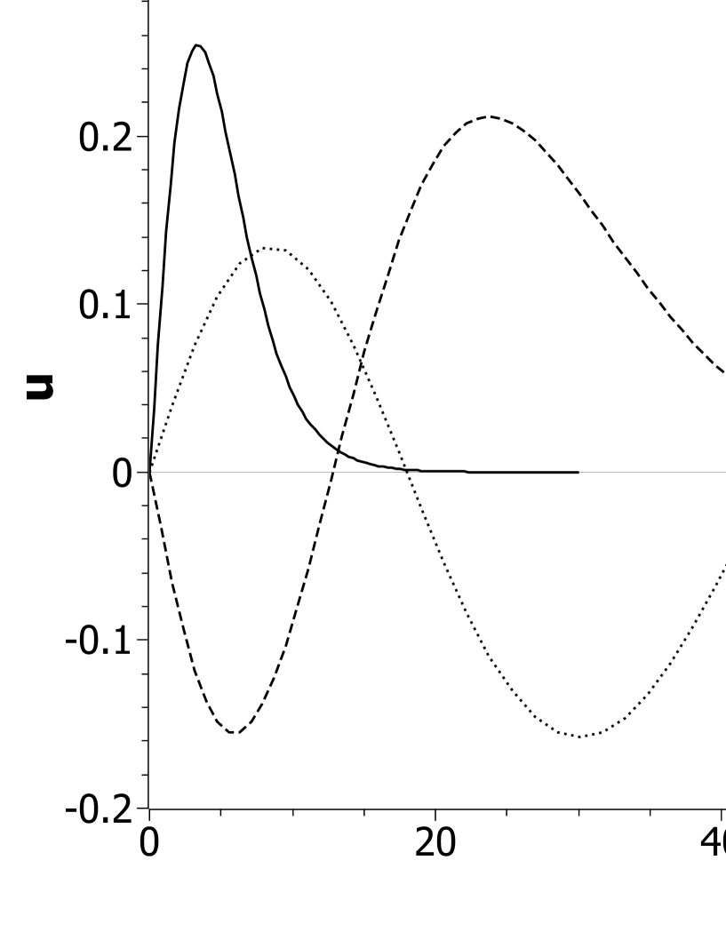
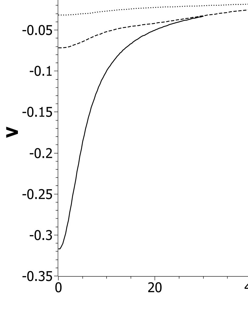
We compute not only the lowest state but also radial excitations, for which the potential is again obtained self consistently and therefore different for each state.³³3For perturbations of these solitons, see [18]. Our results are consistent with earlier calculations [4, 5, 6, 7, 8]. Table 1 lists the results for the ground state and the lowest two radial excitations. Figures 1 and 2 show the modified radial wave function $u$ and the shape of the gravitational potential $V$ for these same cases. However, our main purpose is to compare with a fully relativistic calculation, which we consider in the next section.

Table 1: Energy eigenvalues in units of

G^{2}m^{5}

for the nonrelativistic (NR) Schrödinger–Newton solitons and the relativistic Einstein–Klein–Gordon solitons, the latter being associated with various values of the rescaled Schwarzschild radius

\zeta_{S}=2G^{2}m^{4}

. Here

G

is Newton’s gravitational constant and

m

is the mass associated with the self-gravitating field. For the relativistic results, ‘PF’ indicates the perfect-fluid model and ‘GR’, the direct general relativistic calculation. Relativistic effects increase with

\zeta_{S}

. Two radial excitations are listed, with

n

the number of radial nodes in the wave function.

$\zeta_{S}$	type	$n=0$	$n=1$	$n=2$
–	NR	-0.1628	-0.0309	-0.0125
0.01	PF	-0.1631	-0.0308	-0.0125
	GR	-0.1631	-0.0308	-0.0125
0.1	PF	-0.1663	-0.0308	-0.0126
	GR	-0.1657	-0.0309	-0.0125
0.2	PF	-0.1701	-0.0311	-0.0126
	GR	-0.1688	-0.0310	-0.0126
0.5	PF	-0.1839	-0.0315	-0.0126
	GR	-0.1795	-0.0313	-0.0126
1.0	PF	-0.2218	-0.0322	-0.0127
	GR	-0.2045	-0.0318	-0.0127

Refer to caption — Figure 1: Plots of the modified radial wave function $u$ in units of $\sqrt{a}$ , with $a$ the gravitational Bohr radius $1/Gm^{3}$ , for the ground-state soliton ( $n=0$ ) and two excited cases ( $n=1,2$ ), all for the nonrelativistic Schrödinger–Newton problem. Here $n$ is the number of radial nodes. The associated energies are listed in the first row of Table 1. The dimensionless radial coordinate $\zeta$ is rescaled by $a$ .

III Einstein–Klein–Gordon solitons

III.1 Klein–Gordon equation in curved spacetime

For a proper representation of gravity in a relativistic formulation, we must of course invoke spacetime curvature as represented by a metric $g_{\mu\nu}$ . We are interested in static, spherically symmetric solitons, which means that the metric must have this symmetry. The KG equation for a scalar particle of mass $m$ in this curved spacetime is

\frac{1}{\sqrt{-g}}\partial_{\mu}\left[\sqrt{-g}g^{\mu\nu}\partial_{\nu}\Psi(x)\right]+m^{2}\Psi=0.

(10)

We choose spherical coordinates such that $g_{\mu\nu}$ is diagonal and the line element is

ds^{2}=g_{00}dt^{2}-g_{rr}dr^{2}-r^{2}d\theta^{2}-r^{2}\sin^{2}\theta d\phi^{2},

(11)

for which $g\equiv{\rm det}[g_{\mu\nu}]=-g_{00}g_{rr}r^{4}\sin^{2}\theta$ , with $g_{00}$ and $g_{rr}$ functions only of the radial coordinate $r$ . The KG equation then takes the form

	$\displaystyle\frac{1}{\tilde{g}r^{2}\sin\theta}\left[\frac{\partial}{\partial t}\left(\frac{\tilde{g}r^{2}\sin\theta}{g_{00}}\frac{\partial\Psi}{\partial t}\right)\right.$	$\displaystyle-$	$\displaystyle\frac{\partial}{\partial r}\left(\frac{\tilde{g}r^{2}\sin\theta}{g_{rr}}\frac{\partial\Psi}{\partial r}\right)-\frac{\partial}{\partial\theta}\left(\tilde{g}\sin\theta\frac{\partial\Psi}{\partial\theta}\right)$
			$\displaystyle-\left.\frac{\partial}{\partial\phi}\left(\frac{\tilde{g}}{\sin\theta}\frac{\partial\Psi}{\partial\phi}\right)\right]+m^{2}\Psi=0,$

where⁴⁴4For the Schwarzschild metric, $\tilde{g}=1$ . In [19] this was incorrectly assumed true for other computed metrics, making any non-Schwarzschild results there only qualitative. $\tilde{g}\equiv\sqrt{g_{00}g_{rr}}$ so that $\sqrt{-g}=\tilde{g}r^{2}\sin\theta$ . For a static metric and $\tilde{g}$ independent of angles, this reduces to

\frac{1}{g_{00}}\frac{\partial^{2}\Psi}{\partial t^{2}}-\frac{1}{\tilde{g}r^{2}}\frac{\partial}{\partial r}\left(\frac{\tilde{g}r^{2}}{g_{rr}}\frac{\partial\Psi}{\partial r}\right)+\frac{L^{2}}{r^{2}}\Psi+m^{2}\Psi=0,

(13)

with the usual definition of $L^{2}$ as

L^{2}\equiv-\left[\frac{1}{\sin\theta}\frac{\partial}{\partial\theta}\left(\sin\theta\frac{\partial}{\partial\theta}\right)+\frac{1}{\sin^{2}\theta}\frac{\partial^{2}}{\partial\phi^{2}}\right].

(14)

We then apply separation of variables with $\Psi=\tau(t)R_{l}(r)Y_{lm}(\theta,\phi)$ and isolate the $t$ and $r$ dependence as

\frac{1}{\tau}\frac{d^{2}\tau}{dt^{2}}=\frac{g_{00}}{\tilde{g}r^{2}R_{l}}\frac{d}{dr}\left(\frac{\tilde{g}r^{2}}{g_{rr}}\frac{dR_{l}}{dr}\right)-\left[\frac{l(l+1)}{r^{2}}+m^{2}\right]g_{00}\equiv-E^{2}.

(15)

Here $-E^{2}$ is the separation constant with $E$ obviously interpreted as an energy and $E-m$ the binding energy. The time-dependent $\tau$ function is just $e^{\pm iEt}$ .

We focus on the radial equation:

-\frac{1}{\tilde{g}r^{2}}\frac{d}{dr}\left(\frac{\tilde{g}r^{2}}{g_{rr}}\frac{dR_{l}}{dr}\right)+\frac{l(l+1)}{r^{2}}R_{l}+m^{2}R_{l}=\frac{E^{2}}{g_{00}}R_{l}.

(16)

To facilitate the numerical solution of this equation, we wish to eliminate any first-derivative terms; a finite-difference approximation will then yield a symmetric matrix representation. To accomplish this, we introduce a modified radial wave function $u_{l}(r)\equiv h(r)R_{l}(r)$ with $h(r)$ chosen to eliminate any first-derivative terms in

\frac{d}{dr}\left(\frac{\tilde{g}r^{2}}{g_{rr}}\frac{dR_{l}}{dr}\right)=\frac{d}{dr}\left(\frac{\tilde{g}r^{2}}{g_{rr}h}\right)\left(\frac{du_{l}}{dr}-\frac{h^{\prime}}{h}u_{l}\right)+\frac{\tilde{g}r^{2}}{g_{rr}h}\left(\frac{d^{2}u_{l}}{dr^{2}}-\frac{h^{\prime}}{h}\frac{du_{l}}{dr}+\frac{(h^{\prime})^{2}}{h^{2}}u_{l}-\frac{h^{\prime\prime}}{h}u_{l}\right).

(17)

The coefficient of $\frac{du_{l}}{dr}$ is set to zero:

\frac{d}{dr}\left(\frac{\tilde{g}r^{2}}{g_{rr}h}\right)-\frac{\tilde{g}r^{2}}{g_{rr}h}\frac{h^{\prime}}{h}=0.

(18)

Except for a multiplicative constant, the solution is

h=r\sqrt{\frac{\tilde{g}}{g_{rr}}}.

(19)

The constant in $h$ is irrelevant, given that $h$ appears only in ratios, or can be viewed as absorbed into the normalization of $u_{l}$ . The condition (18) on $h$ also eliminates two terms proportional to $u_{l}$ , leaving

\frac{d}{dr}\left(\frac{\tilde{g}r^{2}}{g_{rr}}\frac{dR_{l}}{dr}\right)=\frac{\tilde{g}r^{2}}{g_{rr}h}\left(\frac{d^{2}u_{l}}{dr^{2}}-\frac{h^{\prime\prime}}{h}u_{l}\right).

(20)

This provides a relatively simple equation for $u_{l}$ :

-\frac{d^{2}u_{l}}{dr^{2}}+\frac{h^{\prime\prime}}{h}u_{l}+\left[\frac{l(l+1)}{r^{2}}+m^{2}\right]g_{rr}u_{l}=\frac{g_{rr}}{g_{00}}E^{2}u_{l}.

(21)

Solutions of this and the original radial equation for a fixed metric, particularly the Schwarzschild metric, have been considered numerically [19] and analytically [20, 21, 22, 23, 24].

The normalization condition is

1=\int_{0}^{\infty}|R_{l}|^{2}\sqrt{g_{rr}}r^{2}\,dr=\int_{0}^{\infty}|u_{l}|^{2}\frac{g_{rr}}{\sqrt{g_{00}}}dr.

(22)

The probability density is

\rho_{lm}=|R_{l}|^{2}|Y_{lm}|^{2}=\frac{|u_{l}|^{2}}{h^{2}}|Y_{lm}|^{2}.

(23)

III.2 Perfect-fluid approximation

To generate a spherically symmetric metric from a mass density $m\rho_{lm}$ , we consider only $l=0$ and define the mass density as

\rho(r)=\frac{m|u_{o}|^{2}}{4\pi h^{2}}.

(24)

This mass density is the source for the computation of the metric. When viewed as a self-consistent solution in a Hartree approximation to a many-body bosonic state, this density can be modeled as a perfect fluid in hydrostatic equilibrium. The metric is then determined by the TOV equation [14, 15, 12, 13] for the pressure $p(r)$

\frac{dp}{dr}=-G\frac{[\rho(r)+p(r)][\mu(r)+4\pi r^{3}p(r)]}{r[r-2G\mu(r)]},

(25)

with the mass function

\mu(r)\equiv 4\pi\int_{0}^{r}\rho(r^{\prime})r^{\prime 2}dr^{\prime}.

(26)

For the spherically symmetric static case, the GR equations are then satisfied by solutions of the form [13]

g_{00}=e^{2A(r)},\;\;g_{rr}=\frac{1}{1-2G\mu(r)/r},

(27)

with the metric function $A(r)$ determined by

\frac{dA}{dr}=G\frac{\mu(r)+4\pi r^{3}p(r)}{r[r-2G\mu(r)]}.

(28)

These three equations, (25), (26), and (28), form a coupled set of integro-differential equations for the metric components with the boundary conditions $\mu(0)=0$ , $A(r)\sim\ln\sqrt{1-2G\mu(r)/r}$ , $p(\infty)=0$ . The form of $A$ applies for $r$ large enough that $\rho$ is effectively zero and all of the mass is contained. The mass function $\mu$ does not reach $m$ even at this range because the fluid structure implicitly assumes internal gravitational binding energy. Thus $\mu(\infty)$ is equal to the mass $m$ minus the gravitational binding energy of the fluid, and $\mu$ is computed without a curvature contribution to the Jacobian [12].

Just as for the nonrelativistic case, there is a natural length scale, the gravitational Bohr radius $a=1/Gm^{3}$ , and an energy scale $G^{2}m^{5}$ . From the latter we define the dimensionless energy parameter $\epsilon$ in terms of the binding energy

\Delta E=E-m=\frac{Gm^{2}}{a}\epsilon=G^{2}m^{5}\epsilon.

(29)

Unlike the nonrelativistic case, there is another length scale, the Schwarzschild radius $r_{S}=2Gm$ . Therefore, in addition to the rescaled radial coordinate $\zeta\equiv r/a$ , we define a dimensionless Schwarzschild radius $\zeta_{S}=r_{S}/a=2G^{2}m^{4}$ . As shown in [19] and reproduced in Appendix A, the magnitude of $\zeta_{S}$ determines the importance of relativistic effects.

These parameters can be used to rescale the coupled system of equations, including the reduced KG equation, which must be solved self consistently. We define

\tilde{u}_{l}=\sqrt{a}u_{l},\;\;\tilde{h}=h/a,\;\;\tilde{\rho}=\frac{4\pi a^{3}}{3m}\rho=\frac{|\tilde{u}_{0}|^{2}}{3\tilde{h}^{2}},

(30)

and

\tilde{\mu}(\zeta)=\frac{\mu(a\zeta)}{m}=\int_{0}^{\zeta}|\tilde{u}_{0}|^{2}\sqrt{\frac{g_{rr}}{g_{00}}}d\zeta^{\prime},\;\;\tilde{p}(\zeta)=\frac{4\pi a^{3}}{3m}p(a\zeta).

(31)

The function $A$ is already dimensionless. The full coupled system of equations becomes⁵⁵5In Eq. (16) of [19], which is the equivalent of the first equation here for general $l$ , there is an $m^{2}$ factor that should be $2/\zeta_{S}$ instead. Also, the terms on the right are slightly different because here the energy scale is larger by a factor of 2, to be consistent with earlier work on the Schrödinger–Newton problem [8].

-\frac{d^{2}\tilde{u}_{0}}{d\zeta^{2}}+\left[\frac{\tilde{h}^{\prime\prime}}{\tilde{h}}+\frac{2}{\zeta_{S}}g_{rr}\left(1-\frac{1}{g_{00}}\right)\right]\tilde{u}_{0}=\left(2\epsilon+\zeta_{S}\frac{\epsilon^{2}}{2}\right)\frac{g_{rr}}{g_{00}}\tilde{u}_{0},

(32)

\frac{d\tilde{\mu}}{d\zeta}=|\tilde{u}_{0}|^{2}\sqrt{\frac{g_{rr}}{g_{00}}},\;\;\tilde{\mu}(0)=0,

(33)

\frac{d\tilde{p}}{d\zeta}=-\frac{\zeta_{S}}{2}\frac{[\tilde{\rho}(\zeta)+\tilde{p}(\zeta)][\tilde{\mu}(\zeta)+3\zeta^{3}\tilde{p}(\zeta)]}{\zeta[\zeta-\zeta_{S}\tilde{\mu}(\zeta)]},\;\;\tilde{p}(\infty)=0,

(34)

and

\frac{dA}{d\zeta}=\frac{\zeta_{S}}{2}\frac{\tilde{\mu}(\zeta)+3\zeta^{3}\tilde{p}(\zeta)}{\zeta[\zeta-\zeta_{S}\tilde{\mu}(\zeta)]},\;\;A\sim\ln\sqrt{1-\zeta_{S}\tilde{\mu}(\zeta)/\zeta},

(35)

with

g_{00}=e^{2A},\;\;g_{rr}=\frac{1}{1-\zeta_{s}\tilde{\mu}(\zeta)/\zeta},

(36)

and the double prime in $\tilde{h}^{\prime\prime}$ meaning $d^{2}\tilde{h}/d\zeta^{2}$ .

This system is solved self consistently starting from an initial guess for the metric, taken as flat inside $\zeta_{S}$ and the Schwarzschild metric with radius $\zeta_{S}$ for $\zeta>\zeta_{S}$ . The KG equation (32) is solved for $\tilde{u}_{0}$ and $\epsilon$ . This determines a guess for the density for which the mass and pressure functions are computed by outward and inward integration of (33) and (34), respectively. Finally, (35) can be integrated inward to find $A$ . The expressions in (36) can then be evaluated to determine an improved metric. The cycle begins again and iterates until convergence to an appropriate tolerance. Some further details of the numerical calculation are given in Appendix B.

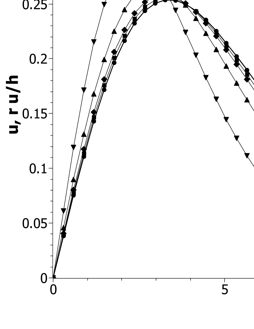
The results for eigenenergies are listed in Table 1, with the type designated as ‘PF’. As $\zeta_{S}$ is increased, the states become more deeply bound, particularly for the ground state. This is consistent with the change in the probability amplitudes, plotted in Figs. 3, where the peaks are shifted toward $\zeta=0$ as $\zeta_{S}$ is increased. It is also consistent with the analysis by Brizuela and Duran-Cabacés [16] of relativistic corrections to the nonrelativistic case, showing that the self-gravitation is increased. For small $\zeta_{S}$ , the amplitudes agree with the nonrelativistic amplitudes, the two being indistinguishable in the plot. For radial excitations the relativistic effects are far less, and the amplitudes all match the nonrelativistic shape for the full range of $\zeta_{S}$ values considered.

III.3 Direct general relativistic calculation

The GR field equations $G_{\mu\nu}=8\pi GT_{\mu\nu}$ can be solved directly in this static, spherically symmetric case. The stress-energy tensor for the scalar field is [10]

T_{\mu\nu}=\frac{1}{2m}\left[(\partial_{\mu}\Psi)(\partial_{\nu}\Psi^{*})+(\partial_{\mu}\Psi^{*})(\partial_{\nu}\Psi)-g_{\mu\nu}(\partial^{\lambda}\Psi)(\partial_{\lambda}\Psi^{*})\right]-g_{\mu\nu}\frac{m^{2}}{2}|\Psi|^{2}.

(37)

Given this as the source, with $\Psi=R(r)e^{\pm iEt}/\sqrt{4\pi}$ , and the metric coefficients written as

g_{00}=e^{2A(r)}\;\;\mbox{and}\;\;g_{rr}=e^{2B(r)},

(38)

the field equations become [10]

e^{2A}\left[\frac{1}{r^{2}}-e^{-2B}\left(\frac{1}{r^{2}}-\frac{2}{r}B^{\prime}\right)\right]=2G\left[e^{2A}|R|^{2}+\frac{1}{2m}e^{2(A-B)}|R^{\prime}|^{2}+\frac{E^{2}}{2m}|R|^{2}\right],

(39)

\frac{1}{r^{2}}(1-e^{2B})+\frac{2}{r}A^{\prime}=2G\left[-\frac{m}{2}e^{2B}|R|^{2}+\frac{1}{2m}|R^{\prime}|^{2}+\frac{E^{2}}{2m}e^{2(B-A)}|R|^{2}\right],

(40)

	$\displaystyle r^{2}e^{-2B}\left[(A^{\prime})^{2}-A^{\prime}B^{\prime}+A^{\prime\prime}+\frac{A^{\prime}-B^{\prime}}{r}\right]$	$\displaystyle=$	$\displaystyle 2G\left[-\frac{m}{2}r^{2}\|R\|^{2}-\frac{r^{2}}{2m}e^{-2B}\|R^{\prime}\|^{2}\right.$
			$\displaystyle\rule{72.26999pt}{0.0pt}\left.+\frac{r^{2}E^{2}}{2m}e^{-2A}\|R\|^{2}\right].$

Here a prime indicates differentiation with respect to $r$ . The KG equation for $R$ , Eq. (16), can be written in terms of the same metric functions as

-R^{\prime\prime}-\left[\frac{2}{r}+A^{\prime}-B^{\prime}\right]R^{\prime}+m^{2}e^{2B}R=E^{2}e^{2(B-A)}R.

(42)

The third GR equation, Eq. (III.3), can be derived from this radial KG equation and the first two GR equations.

The dimensionless forms of the first two GR equations are

	$\displaystyle\frac{dA}{d\zeta}$	$\displaystyle=$	$\displaystyle\frac{1}{2\zeta}(e^{2B}-1)-\frac{\zeta_{S}\zeta}{4}e^{2B}\tilde{R}^{2}+\frac{\zeta_{S}^{2}\zeta}{8}\left(\frac{d\tilde{R}}{d\zeta}\right)^{2}+\frac{\zeta_{S}\zeta}{4}\left[1+\frac{1}{2}\zeta_{S}\epsilon\right]^{2}e^{2(B-A)}\tilde{R}^{2},$		(43)
	$\displaystyle\frac{dB}{d\zeta}$	$\displaystyle=$	$\displaystyle-\frac{1}{2\zeta}(e^{2B}-1)+\frac{\zeta_{S}\zeta}{4}e^{2B}\tilde{R}^{2}+\frac{\zeta_{S}^{2}\zeta}{8}\left(\frac{d\tilde{R}}{d\zeta}\right)^{2}+\frac{\zeta_{S}\zeta}{4}\left[1+\frac{1}{2}\zeta_{S}\epsilon\right]^{2}e^{2(B-A)}\tilde{R}^{2},$		(44)

with $\tilde{R}=a^{3/2}R=\tilde{u}/\tilde{h}$ . Given the radial function $\tilde{u}$ , these equations can be solved numerically for the metric functions $A$ and $B$ , and the radial KG equation is solved self consistently.

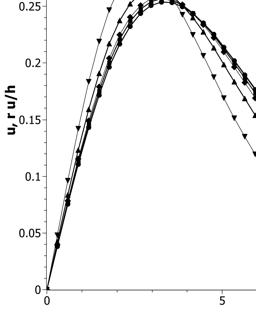
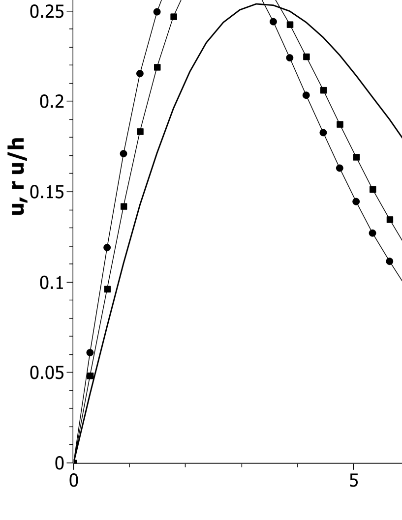
The result for the energy eigenvalues $\epsilon$ are listed in Table 1, designated as the type ‘GR’. Except for the largest value of $\zeta_{S}$ , they are not significantly different from those of the perfect-fluid model. The wave functions are plotted in Fig. 4 and, for $\zeta_{S}=1$ , compared with the wave function in the perfect-fluid model in Fig. 5. Again, the ground state in the relativistic case is more deeply bound, but not as much as in the perfect-fluid model; this can be seen explicitly in Fig. 5 and Table 1.

IV Summary

We have shown that the relativistic version of the Schrödinger–Newton problem for scalar particles can be solved for Einstein–Klein–Gordon solitons in spherically symmetric spacetimes. This includes radial excitations. We consider both a perfect-fluid model, consistent with a Hartree approximation to a bosonic star, and the fundamental GR equations with the stress-tensor of the KG field. The results for the Schrödinger–Newton problem are recovered in the nonrelativistic limit, which is controlled by the ratio of the Schwarzschild radius to the gravitational Bohr radius for the given mass.

The eigenenergies obtained are listed in Table 1. The relativistic cases are more deeply bound than the nonrelativistic case, particularly for the ground state. This can also be seen in the amplitudes, as plotted in Figs. 3, 4, and 5, where the relativistic peaks occur at smaller radii. This is consistent with the findings of Brizuela and Duran-Cabacés [16] in their analysis of relativistic corrections to the nonrelativistic Schrödinger–Newton problem. We also find that the perfect-fluid model binds more deeply than occurs for the fundamental GR equations that use only the stress-energy tensor of the scalar field. Apparently, the additional assumption of hydrostatic equilibrium increases the energy density and consequently the spatial curvature.

The restriction to spherical symmetry can be relaxed to consider cylindrical symmetry. This has been done at least partially for the Schrödinger–Newton problem [8], though with an unnecessary assumption of a cylindrically symmetric wave function with $L_{z}=0$ . A more complete nonrelativistic calculation could be done as well as consideration of a relativistic formulation [25].

Our approach represents a form of semi-classical gravity where the matter fields are treated quantum mechanically but gravity classically. It requires self-consistent solutions for the metric and the quantum particle amplitude. The results of such computations may provide a check on the structure of a theory of quantum gravity.

Acknowledgements.

This work was supported in part by the Minnesota Supercomputing Institute and the Research Computing and Data Services at the University of Idaho through grants of computing time.

Appendix A Nonrelativistic limit

For completeness, we repeat the argument from [19] that $\zeta_{S}$ controls the importance of relativistic effects. For simplicity, we consider the Schwarzschild geometry, for which $g_{00}=1-2Gm/r=1-\zeta_{S}/\zeta=1/g_{rr}$ . In this case, we have $\tilde{g}=\sqrt{g_{00}g_{rr}}=1$ and $h=r/\sqrt{g_{rr}}=a\zeta/\sqrt{g_{rr}}$ . The $\tilde{h}^{\prime\prime}/\tilde{h}$ term in the modified KG equation (32) is then

\frac{\tilde{h}^{\prime\prime}}{\tilde{h}}=-\frac{\zeta_{S}^{2}}{4\zeta^{2}(\zeta^{2}-\zeta_{S}^{2})},

(45)

and the modified radial equation becomes

-\frac{d^{2}\tilde{u}_{0}}{d\zeta^{2}}-\frac{1}{4}\frac{\zeta_{S}^{2}}{\zeta^{2}(\zeta-\zeta_{S})^{2}}\tilde{u}_{0}-\frac{2}{\zeta}\frac{1}{(1-\zeta_{S}/\zeta)^{2}}\tilde{u}_{0}=\frac{2\epsilon+\frac{1}{2}\zeta_{S}\epsilon^{2}}{(1-\zeta_{S}/\zeta)^{2}}\tilde{u}_{0}.

(46)

Keeping $\zeta_{S}$ to first order, we obtain

-\frac{d^{2}\tilde{u}_{0}}{d\zeta^{2}}-\frac{2}{\zeta}(1+2\zeta_{S}/\zeta)\tilde{u}_{0}=(2\epsilon(1+2\zeta_{S}/\zeta)+\frac{1}{2}\zeta_{S}\epsilon^{2})\tilde{u}_{0},

(47)

which can be rearranged as

-\frac{d^{2}\tilde{u}_{0}}{d\zeta^{2}}-\frac{2}{\zeta}\tilde{u}_{0}-\zeta_{S}\left[\frac{4}{\zeta^{2}}-\frac{4\epsilon}{\zeta}+\frac{1}{2}\epsilon^{2}\right]\tilde{u}_{0}=2\epsilon\tilde{u}_{0}.

(48)

The $\zeta_{S}$ terms are then revealed to be corrections to the ordinary Coulomb problem of Newtonian gravity.

Appendix B Details of the numerical calculation

Just as for the nonrelativistic case, the infinite range of the radial coordinate is truncated at a distant point and the density and pressure are assumed to be zero beyond that point. The scaled KG equation is represented by a matrix equation obtained from finite-difference approximations to the derivatives of $\tilde{u}_{0}$ and $\tilde{h}$ on an equally spaced grid. The metric is then computed on this grid by solving the first-order equations for $\tilde{\mu}$ , $\tilde{p}$ and $A$ in the perfect-fluid model, or for $A$ and $B$ in the fundamental GR equations, with a second-order Runge–Kutta method, utilizing a matching step size. This choice has an error term consistent with the chosen finite-difference approximation to the KG equation. For better accuracy, one could of course use higher order methods, but these were sufficient for the purpose of comparing the nonrelativistic and relativistic results, with approximately four significant figures in the values of scaled energies.

In order that the matrix representation of the KG equation be symmetric, we introduce a new function $\bar{u}\equiv\tilde{u}\sqrt{g_{rr}/g_{00}}$ and multiply (32) by $\sqrt{g_{rr}/g_{00}}$ . We also define $\lambda\equiv 2\epsilon+\zeta_{S}\epsilon^{2}/2$ as the direct eigenvalue of the matrix. The differential equation solved numerically to obtain the KG eigenstates is actually

-\sqrt{\frac{g_{00}}{g_{rr}}}\frac{d^{2}}{d\zeta^{2}}\left[\sqrt{\frac{g_{00}}{g_{rr}}}\bar{u}\right]+\frac{g_{00}}{g_{rr}}\frac{\tilde{h}^{\prime\prime}}{\tilde{h}}\bar{u}+\frac{2}{\zeta_{S}}g_{00}\left[1-\frac{1}{g_{00}}\right]\bar{u}=\lambda\bar{u}.

(49)

The third term on the left-hand side is best evaluated as $2e^{A}\sinh A$ , which comes from $g_{00}=e^{2A}$ , rather than in its explicit form, because $g_{00}$ can be close to 1. Also, the scaled binding energy is best extracted from $\lambda$ by a rearrangement of the quadratic formula

\epsilon=\frac{\lambda}{1+\sqrt{1+\zeta_{s}\lambda/2}}.

(50)

References

[1] R. Ruffini and S. Bonazzola, Systems of self-gravitating particles in general relativity and the concept of an equation of state, Phys. Rev. 187, 5 (1969).
[2] L. Diósi, Gravitation and quantum-mechanical localization of macro-objects, Phys. Lett. A 105, 5 (1984).
[3] R. Penrose, On gravity’s role in quantum state reduction, Gen. Rel. Grav. 28, 581 (1996).
[4] I.M. Moroz, R. Penrose, and K.P. Tod, Spherically symmetric solutions of the Schrödinger–Newton equations, Class. Quant. Grav. 15, 2733 (1998).
[5] D.H Bernstein, E. Giladi, and K.R.W. Jones, Eigenstates of the gravitational Schrödinger equation, Mod. Phys. Lett. A 13, 29 (1998).
[6] K.P. Tod, The ground state energy of the Schrödinger–Newton equation, Phys. Lett. A 280, 4 (2001).
[7] R. Harrison, I.M. Moroz, and K.P. Tod, A numerical study of the Schrödinger–Newton equations, Nonlinearity 16, 1 (2002).
[8] R. Harrison, A numerical study of the Schrödinger–Newton equations, Ph.D. Thesis, University of Oxford, 2001, unpublished.
[9] R. Bahrami, A. Großardt, S. Donadi, and A. Bassi, The Schrödinger–Newton equation and its foundations, New J. Phys. 16, 115007 (2014).
[10] D. Giulini and A. Großardt, The Schrödinger–Newton equation as a nonrelativistic limit of self-gravitating Klein–Gordon and Dirac fields, Class. Quant. Grav. 29, 215010 (2012).
[11] B. Kain, “Einstein–Dirac system in semiclassical gravity,” Phys. Rev. D 107, 124001 (2023).
[12] S.M. Carroll, Spacetime and Geometry: An Introduction to General Relativity, (Cambridge University Press, Cambridge, 2019).
[13] J.B. Griffiths and J. Podolsky, Exact Spacetimes in Einstein’s General Relativity, (Cambridge University Press, Cambridge, 2009).
[14] R.C. Tolman, Static solutions of Einstein’s field equations for spheres of fluid, Phys. Rev. 55, 364 (1939).
[15] J.R. Oppenheimer and G.M. Volkov, On massive neutron cores, Phys. Rev. 55, 374 (1939).
[16] D. Brizuela and A. Duran-Cabacés, Relativistic effects on the Schrödinger–Newton equation, Phys. Rev. D 106, 124038 (2022).
[17] F.S. Guzmán and L.A. Ureña-López, Gravitational atoms: General framework for the construction of multistate axially symmetric solutions of the Schrödinger–Poisson system, Phys. Rev. D 101, 081392 (2020).
[18] J. Luna Zagorac, I. Sands, N. Padmanabhan, and R. Easther, Schrödinger–Poisson solitons: Perturbation theory, Phys. Rev. D 105, 103506 (2022).
[19] R.D. Lehn, S.S. Chabysheva, and J.R. Hiller, Klein–Gordon equation in curved space-time, Eur. J. Phys. 39, 045405 (2018).
[20] P.D.P. Smith, Use of the Schwarzschild metric in the Klein-Gordon equation, Phys. Lett. A 43, 144 (1973).
[21] D.J. Rowan and G. Stephenson, Solutions of the time-dependent Klein-Gordon equation in a Schwarzschild background space, J. Phys. A: Math. Gen. 9, 1631 (1976).
[22] E. Elizalde, Series solutions for the Klein–Gordon equation in Schwarzschild space-time, Phys. Rev. D 36, 1269 (1987); Exact solutions of the massive Klein–Gordon–Schwarzschild equation, Phys. Rev. D 37, 2127 (1988).
[23] Y.P. Qin, Exact solutions to the Klein-Gordon equation in the vicinity of Schwarzschild black holes, Sci. China Phys. Mech. Astron. 55, 381 (2012).
[24] W.-D. Li, Y.-Z. Chen, and W.-S. Dai, Scattering state and bound state of scalar field in Schwarzschild spacetime: Exact solution, Ann. Phys. 409, 167919 (2019).
[25] K. Bronnikov, N. O. Santos, and A. Wang, “Cylindrical systems in general relativity,” Class. Quant. Grav. 37, 113002 (2020).

Gravitational soliton solutions to self-coupled Klein-Gordon and Schrödinger equations