GraphHop: An Enhanced Label Propagation Method for Node Classification
Abstract
A scalable semi-supervised node classification method on graph-structured data, called GraphHop, is proposed in this work. The graph contains attributes of all nodes but labels of a few nodes. The classical label propagation (LP) method and the emerging graph convolutional network (GCN) are two popular semi-supervised solutions to this problem. The LP method is not effective in modeling node attributes and labels jointly or facing a slow convergence rate on large-scale graphs. GraphHop is proposed to its shortcoming. With proper initial label vector embeddings, each iteration of GraphHop contains two steps: 1) label aggregation and 2) label update. In Step 1, each node aggregates its neighbors’ label vectors obtained in the previous iteration. In Step 2, a new label vector is predicted for each node based on the label of the node itself and the aggregated label information obtained in Step 1. This iterative procedure exploits the neighborhood information and enables GraphHop to perform well in an extremely small label rate setting and scale well for very large graphs. Experimental results show that GraphHop outperforms state-of-the-art graph learning methods on a wide range of tasks (e.g., multi-label and multi-class classification on citation networks, social graphs, and commodity consumption graphs) in graphs of various sizes. Our codes are publicly available on GitHub 111https://github.com/TianXieUSC/GraphHop.
Index Terms:
Graph learning, semi-supervised learning, label propagation, graph convolutional networks, large-scale graphs.I Introduction
The success of deep learning and neural networks often comes at the price of a large number of labeled data. Semi-supervised learning is an important paradigm that leverages a large number of unlabeled data to address this limitation. The need for semi-supervised learning has arisen in many machine learning problems and found wide applications in computer vision, natural language processing, and graph-based modeling, where getting labeled data is expensive and there exists a large amount of unlabeled data.
Among semi-supervised graph learning methods, label propagation (LP) [1, 2] has demonstrated good adaptability, scalability, and efficiency for node classification. Fig. 1 gives a toy example of LP on a graph, where data entities are represented by nodes and edges are either formed with pairwise similarities of linked nodes or generated by a certain relationship (e.g., social networks). LP exploits the geometry of data entities induced by labeled and unlabeled examples. With fewer labeled nodes, LP iteratively aggregates label embeddings from neighbors and propagates them throughout the graph to provide labels for all nodes. Typically, LP-based techniques have a small memory requirement [3] and a fast convergence rate. On the other hand, LP-based methods are limited in their capability of integrating multiple data modalities for effective learning. Nodes in a graph may contain attributes and class labels. Only propagating the label information may not be adequate. Take the node classification problem for citation networks as an example. Each paper is represented as a node with a bag-of-words attribute vector that describes its keywords and associated class label. Edges in the graph are formed by citation links between papers. The three pieces of information (i.e., node attributes, node labels, and edges) should be jointly considered to make accurate node classification. Furthermore, the rules of label propagation in LP methods are often implemented by a simple lookup table for unlabeled nodes. They fail to leverage the label information in a probabilistic way.

Due to the recent success of neural networks [4], there has been an effort of applying neural networks into graph-structured data. One pioneering technique, known as graph convolutional networks (GCNs) [5], has achieved impressive node classification performance for citation networks. Instead of propagating label embeddings as done by LP, GCNs conduct attributes propagation through a graph with labels as supervision. On one hand, GCNs incorporate node attributes, node labels, and edges in model learning. On the other hand, GCNs fail to exploit the label distribution in the graph structure. Reliance on labels as supervision limits label update efficiency and hinders the ability in an extremely small label rate scenario, e.g. only one labeled example per class. Li, et al. [6] proposed a new method called label efficient GCNs. However, their method does not induce unlabeled data but only changes the convolutional filters in model learning. Others [7, 8, 9] tried to incorporate label distributions in a generative model based on special inductive bias assumptions [10]. Furthermore, end-to-end training makes neural-network-based solutions difficult to scale for large graphs. The rapid expansion of neighborhood sizes along deeper layers restricts GCNs from batch training [11]. There is a trade-off between training efficiency and the receptive field size [12].
To address the weaknesses of LP and GCNs, a scalable semi-supervised graph learning method, called GraphHop, is proposed in this work. GraphHop fully exploits node attributes, labels, and link structures for graph-structured data learning. Node attributes and labels are viewed as signals, which are assumed to be locally smooth on graphs. Attributes exist in all nodes while labels are only available in a small number of nodes (i.e., a typical semi-supervised setting). GraphHop integrates two signal types based on an iterative learning process. Node attributes are used to predict the label embedding vector at each node in the initialization stage. The dimension of the label embedding vector is the same as the class number, where each element indicates the probability of belonging to a class. After initialization, each iteration of GraphHop contains two steps: 1) label aggregation and 2) label update. In Step 1, each node aggregates its neighbors’ label embedding vectors obtained in the previous iteration. In Step 2, a new label embedding vector is predicted for each node based on the label vector of the node itself and the aggregated label vector obtained in Step 1. The iterative procedure exploits multi-hop neighborhood information, leading to the name of “GraphHop”, for efficient learning. It enables GraphHop to perform well in an extremely small label rate setting and scale well for very large graphs. We conduct extensive experiments to validate the effectiveness of the proposed GraphHop method. We test a variety of semi-supervised node classification tasks including multi-class classification on various sizes of graphs and multi-label classification on protein networks. The proposed GraphHop method achieves superiorly in terms of prediction accuracy and training efficiency.
The rest of this paper is organized as follows. Some preliminaries are introduced in Sec. II. The GraphHop method is presented in Sec. III. The adoption of batch training and the small number of parameters makes GraphHop efficient and scalable to large-scale graphs. Theoretical analysis is conducted to estimate the required iteration number of the iterative algorithm in Sec. IV. Extensive experiments are conducted to show the state-of-the-art performance with low memory usage in Sec. V. Comments on related work are made in Sec. VI. Finally, concluding remarks are given and future research directions are pointed out in Sec. VII.
II Preliminaries
In this section, we first formulate the transductive semi-supervised learning problem on graphs in Sec. II-A. Then, we present the smoothness assumption, which holds for most graph learning methods and provides its empirical evidence in Sec. II-B. Finally, we review two commonly used graph signal processing tools in Sec. II-C.

II-A Problem Statement
An undirected graph can be represented by a triple:
| (1) |
where denotes a set of nodes, is the adjacency matrix between nodes, and is the attribute matrix whose -dimensional row vector is an attribute vector associated with each node. In the setting of semi-supervised classification, each labeled node belongs to one class,
Nodes are divided into labeled and unlabeled sets with their indices denoted by
| (2) |
respectively.
Let be the set of matrices with nonnegative entries. Matrix
is the global label embedding matrix. It can be divided into
where and represent labeled and unlabeled examples, respectively. For labeled examples , vector is an one-hot vector, where if is labeled as and otherwise. For unlabeled examples , vector is a probability vector whose element is the predicted probability of belonging to class . To classify unlabeled node in the convergence stage, we assign it the label of the most likely class:
| (3) |
The goal of transductive graph learning is to infer labels of unlabeled nodes (i.e., matrix ), given attribute matrix , adjacency matrix , and labeled examples . In the extremely small label rate case, the number of examples in the labeled set is much smaller than that in the unlabeled set; namely,
II-B Assumption
Both the attribute matrix and the label embedding matrix can be treated as signals on graphs. For example, the -dimensional column vectors of attribute matrix can be viewed as a -channel graph signal. One assumption for semi-supervised learning is that data points that are close in a high density region should have similar attributes and produce similar outputs. This property can be stated qualitatively below.
Assumption 1.
The node attribute and label signals are smooth functions on graphs.
The smoothness of attributes and labels can be verified by evaluating their means and variances as a function of the length of the shortest path between every two nodes, which is usually measured in terms of the hop count. Here, we propose an alternative approach to verify the smooth label assumption and conduct experiments on the Cora, CiteSeer and PubMed datasets (see Sec. V for more details) using the following procedure.
Step 1. Compute the graph Fourier basis
and its corresponding frequency matrix
from graph Laplacian
where frequencies in are arranged in an ascending order:
| (4) |
Similarly, we can define the reverse-ordered frequency matrix,
and find the corresponding basis matrix,
It is well known that the basis signals associated with lower frequencies (i.e., smaller eigenvalues) are smoother on the graph [13].
Step 2. Compute the top- lowest or highest frequency components of labels via
where each row of denotes the one-hot embedding of a node label. Then, we reconstruct labels for all nodes via
Make a prediction based on the reconstructed label embedding matrix, where classes of node are decided by Eq. (3). The above computation yields two classification results for each node - one using smooth components () while the other using highly fluctuating components ().
We add the number of Laplacian frequency components incrementally, reconstruct label embeddings for classification, and show two accuracy curves for each dataset in Fig. 2, where the one using low frequency components is in blue and the one using high frequency components is in red. The blue curve rises up quickly while the red curve increases slowly in all three cases, which support our assumption that label signals are smooth on graphs. Interestingly, the performance does drop when adding more high frequency components for PubMed.
II-C Smoothening Operations
Based on the smoothness assumption of label signals, we expect that a smoothening operation on node attributes and labels helps achieve better classification results. There are several common ways to achieve the smoothening effect, which can be categorized into the following three types.
-
1.
Average attributes or label embedding vectors of neighboring nodes. It is well known that the average operation behaves like a lowpass filter [12]. Another reason for taking the average is that nodes have different numbers of -hop neighbors, denoted by , where . By averaging the attributes/labels of nodes with the same hop distance, we can consider the impact of -hop neighbors for all nodes uniformly.
-
2.
Use regression for label prediction. We need to predict labels for a great majority of nodes based on attributes of all nodes and labels of a few nodes. One way for prediction is to train a regressor. In the current setting, the logistic regression (LR) classifier is a better choice due to the discrete nature of the output. Regression (regardless of a linear or a logistic regressor) is fundamentally a smoothening operation since it adopts a fixed but smaller model size to fit a large number of observations.
- 3.
The LP method can be formally defined as a minimization of cost function
| (5) |
where is the one-hot label embedding matrix of labeled nodes, is the Frobenius norm, is a parameter controlling the degree of the regularization, and is the unnormalized graph Laplacian. The optimization solution of embedding matrix in Eq. (5) can be derived equivalently by applying a embedding propagation process, where the th iteration update is
| (6) |
where and zeros for unlabeled examples. The update rule can be described by replacing the current label embeddings with their averaged neighbors’ through a look up table plus the initially labeled examples. As shown in Eqs. (5) and (6), we see that the LP method exploits smoothening operations of the first and the third types, respectively.
Despite the simple and efficient propagation process in Eq. (6), the LP method is limited in its learning abilities in label embedding vector update in the following three aspects.
-
•
Only label embeddings of immediate (one-hop) neighbors are being propagated at each iteration according to Eq. (6). It could be advantageous to consider label embeddings of nodes in a larger neighborhood.
-
•
The availability of node attributes is not leveraged.
-
•
The current label vectors of unlabeled nodes are fully replaced (Eq. (6)) by propagated embeddings from neighbors of the previous iteration. The simple label update rule limits the ability to learn the correlation of label embeddings between the node itself and its neighbors.

III GraphHop Method
The GraphHop method is introduced in this section. It is an iterative algorithm that contains an initialization stage and an iteration stage as shown in Fig. 3. In the initialization stage, it predicts the initial label embedding vector for all nodes based on attribute vectors via regression. In the iteration stage, it focuses on label propagation and update. No attributes information is needed in the iteration stage and, as a result, its model size is small. In particular, GraphHop has the following novel features to address the limitations of the LP method as described in the last section.
-
•
It exploits both attribute and label embeddings of one- or multi-hop neighbors.
-
•
It leverages the information of node attributes in the initialization stage.
-
•
The label vectors of unlabeled nodes are predicted through regression of (rather than being replaced by) label embeddings from one- or multi-hop neighbors of the previous iteration. The regression-based update rule, which is the smoothening operation of the second type as mentioned above, boosts the learning power of GraphHop.
III-A Initialization
The goal of the initialization stage is to offer good initialize label embedding vectors for all nodes. Recall that the label embedding vector is a -dimensional vector whose elements indicate the probability of a node belonging to class . If a node is a labeled one, its initial embedding is a one-hot (or multi-hot in multi-label classification) vector. If a node has no label, we can train an LR classifier that uses the attributes of the node itself as well its multi-hop neighbors to predict the initial embeddings. This is justified by the underlying assumption of semi-supervised graph learning; namely, nodes of spatial proximity should have similar attributes and produce similar outputs (i.e., labels).
The input to the LR classifier is the averaged attributes of -hops, , where denotes the self node. For node , we have the following averaged attribute vectors of dimension :
| (8) |
where denotes the -hop neighbors of node . This yields an aggregated attribute matrix, , whose -dimensional row vector is the concatenation of these vectors associated with each node. Mathematically, we can express it as
| (9) |
where denotes column-wise concatenation, is the normalized -hop adjacency matrix, and is the hop index. The output of the LR classifier is the initial label embeddings matrix, denoted by , of all nodes. This aggregation procedure is illustrated in Fig. 4.
We first use the labeled examples to determine the model parameters of the LR classifier in the training phase. Afterwards, we use the trained LR classifier to infer the initial label embeddings of unlabeled nodes. Mathematically, this is expressed as
| (10) |
where denotes the predictor based on the LR classifier, is the label embeddings of known examples and is the set of learned model parameters.

III-B Iteration
After initialization, the GraphHop method processes label embedding vectors via a two-step procedure at each iteration as elaborated below.
III-B1 Step 1: Label Aggregation
The label aggregation mechanism is exactly the same as the attribute aggregation mechanism as stated in Sec. III-A. By modifying Eq. (9) slightly, we have the following label aggregation formula
| (11) |
The label aggregation step with is shown in Figs. 3 and 4 as an example, where the green node is the center node, nodes in the red region are one-hop neighbors and nodes in the blue region are two-hop neighbors. The averaged label embeddings of one-hop neighbors and two-hop neighbors yield two output label embedding vectors, respectively. They are concatenated with the label embedding of the center node, which serves as the input to the label update step. As shown in Fig. 3, we can form multiple aggregated outputs and for each used as input to label update step for ensembles. Yet, a larger value results in larger memory and computational complexity. Even with the one-hop connection (i.e., ), the propagation region is still increasing due to iteration. This is not available in the model of [12] (see Eq. (18)). In experiments, we focus on the case with .
III-B2 Step 2: Label Update
A label update operation is conducted on the propagated label embeddings to smoothen the label embeddings furthermore. For traditional LP, the update is formulated as a simple replacement as given in Eq. (6). This update rule does not explore embedding correlations between nodes and their neighbors fully. For improvement, we propose to train the label update operation and view it as a predictor from concatenated label embeddings at iteration to the new label embeddings at iteration . Mathematically, we have
| (12) |
Here, we choose multiple LR classifiers (one for each ) as the predictors and average the predicted label embeddings as shown in Fig. 3. Note that there are many choices for the predictor in Eq. (12), say, [14, 15, 16]. The choice for the LR classifier is because of its efficiency and smaller model size. The implementation details of the LR classifier are elaborated in Appendix A.
Finally, the GraphHop method is summarized by pseudo-codes in Algorithm 1.
IV Analysis
IV-A Convergence Analysis
We analyze the relationship between the lower bound of iteration number, label rate, and the hops number in the label propagation step. The higher-order (large hops) of nodes was efficiently approximated within -hop neighbors in [17]. Here, we call the approximation of each unlabeled node is sufficient if at least one initially labeled examples are captured in its -hop surroundings after iteration, and otherwise insufficient. If all unlabeled nodes are sufficient, we call the iteration sufficient.
We define the shortest distance between nodes and as in the graph. Given initially labeled examples, we partition node set into several subsets
where denotes the set of initially labeled nodes,
is the subset of unlabeled nodes that have the same minimum distance (i.e., of hops) to one of labeled nodes, and is the maximum distance between an unlabeled node and a labeled one. Since each node will aggregate -hop neighbors embeddings at one iteration, we have the following Lemma.
Lemma 1.
Given the maximum hop covered in each label propagation step, the node predictions in will be insufficient until the propagation of iteration is finished.
Based on Lemma 1, we can derive the number of sufficient nodes after iterations.
Theorem 1.
Let be a graph with nodes, and the maximum degree of all nodes in . The number of initially labeled nodes is . Then after iterations, at most nodes are sufficient.
Proof.
Since in semi-supervised learning, we ignore the difference between the number of unlabeled nodes (i.e. )and all nodes in the graph (i.e. ). According to Lemma 1, after iterations, the nodes in subsets , , , are sufficient. Then, we have
| (13) | ||||
The first equality is because that are mutually disjoint. Each node has only one unique minimum distance to labeled set so that they can only be assigned to one specific subset. The inequality is due to the use of the maximum degree for every node. Apparently, . Thus, we get
| (14) |
and the theorem is proved. ∎
It is easy to get the following corollary.
Corollary 1.
The predictions of all unlabeled nodes on graph will be sufficient with iterations, where
| (15) |
Proof.
According to Theorem 1, at most nodes are sufficient after iterations. To ensure that all nodes on graph are sufficient, we let
so that
| (16) |
∎
The result in Corollary 1 shows that the relationship between sufficient iterations and the maximum hop number in is in inverse ratio. Increasing will decrease the required number of iterations. The initial label rate and graph density also have an influence on the iteration number. Yet, the effects are minor due to the logarithm function. Particularly, in a large-scale graph where , changing the label rate has negligible influence on the iteration number. The same behavior has been shown in the experiment section. In practice, we observe that GraphHop converges in few iterations (usually 10) since few iterations are required to achieve sufficiency.
IV-B Complexity Analysis
The time and memory complexities of GraphHop are significantly lower that the traditional training in graph neural networks. The reason is that GraphHop can do minibatch training, which is not available GCN-based methods due to the neighbor expansion problem [11]. The LR classifiers are directly trained based on the output of Eq. (12), where minibatches can be easily applied to matrix (see lines 6 and 16 in Algorithm 1) as input.
Suppose that the total training minibatch number is , the number of iterations is , the minibatch size is , and the number of classes is . Then, the time complexity of one minibatch propagation is
where the first term comes from label aggregation while the second from label update. The memory usage complexity is
which represents one minibatch embeddings and parameters for the classifiers. Note that the parameter size is fixed and independent of iterations and scales linearly in terms of the minibatch size .
V Experiments
We conduct experiments to evaluate the performance of GraphHop with multiple datasets and tasks. Datasets used in the experiments are described in Sec. V-A. Experimental settings are discussed in Sec. V-B. Then, the performance of GraphHop is compared with state-of-the-art methods in small- and large-scale graphs in Sec. V-C. Finally, ablation studies are given in Sec. V-E.
V-A Datasets
We evaluate the performance of GraphHop on six representative graph datasets as shown in Table I. Cora, CiteSeer, and PubMed [5] are three citation networks. Nodes are papers while edges are citation links in these graphs. The task is to predict the category of each paper. PPI and Reddit [18] are two datasets of large-scale networks. PPI is a multi-label dataset, where each node denotes one protein with multiple labels in the gene ontology sets (121 in total). Amazon2M [11] is by far the largest graph dataset that is publicly available with over 2 millions nodes and 61 millions of edges obtained from Amazon co-purchasing networks. The raw node features are bag-of-words extracted from product descriptions. We use the principal component analysis (PCA) [19] to reduce their dimension to . Also, we use the top-level category as the class label for each node.
| Dataset | Vertices | Edges | Classes | Features Dims |
| Cora | ||||
| CiteSeer | ||||
| PubMed | ||||
| PPI | ||||
| Amazon2M |
| Dataset | Data splits | ||||
| Train | Validation | ||||
| PPI | |||||
| Amazon2M | |||||
| Datasets | |||
| Cora | |||
| CiteSeer | |||
| PubMed | |||
| PPI | |||
| Amazon2M |
V-B Experimental Settings
We evaluate GraphHop and several benchmarking methods on the semi-supervised node classification task in a transductive setting at a number of label rates. For citation datasets, we first conduct experiments by following the conventional train/validate/test split (i.e., 20 labels per class) of the training set. Next, we train models at extremely low label rates (i.e., 1, 2, 4, 8, and 16 labeled examples per class). For the PPI, Reddit, and Amazon2M three large-scale networks, the original data splits target at inductive learning scenario, which do not fit our purpose. To tailor them to the transductive semi-supervised setting, we adopt fewer labeled training examples. To be specific, for Reddit and Amazon2M, we pick the same number of examples in each class randomly with multiple label rates for training. For the multi-label PPI dataset, we simply select a small portion of examples randomly in the training. A fixed size of remaining examples is selected as validation while the rest is used as testing. The full data splits are summarized in Table II. For simplicity, we use the percentages of training examples to indicate different data split in reporting performance results.
We implement GraphHop in PyTorch [20]. For the LR classifiers in the initialization stage and the iteration stage, we use the same Adam optimizer with a learning rate of and weight decay. The batch size is fixed to for citation networks but adaptive for large-scale graphs since experiments show there is a trade-off using different batch sizes for the latter case. The training epochs are set to with an early stopping criterion which stops the classifiers from training and goes to the next iteration. We set the maximum iteration to for citation datasets and for large-scale networks. These numbers are large enough for GraphHop to converge as shown in the experiments. For hyperparameters , , and , we perform a grid search in the parameter space based on the validation results. The hyperparameter tuning ranges and their final values are listed in Table III and IV, respectively. Note that hyperparameters are tuned for different label rates. We show their values with respect to the largest label rates in Table IV. All experiments were conducted on a machine with a NVIDIA Tesla P100 GPU (16 GB memory), 10-core Intel Xeon CPU ( GHz), and GB of RAM.
V-C Performance Evaluation
| Cora | Citeseer | Pubmed | ||||||||||||||||
| # of labels per class | 1 | 2 | 4 | 8 | 16 | 20 | 1 | 2 | 4 | 8 | 16 | 20 | 1 | 2 | 4 | 8 | 16 | 20 |
| LP | ||||||||||||||||||
| DeepWalk | - | - | - | - | - | - | ||||||||||||
| LINE | - | - | - | - | - | - | ||||||||||||
| GCN | ||||||||||||||||||
| GAT | - | - | - | - | - | - | ||||||||||||
| DGI | 63.1 | 71.8 | 61.7 | 65.6 | - | - | - | - | - | - | ||||||||
| Graph2Gauss | - | - | - | - | - | - | ||||||||||||
| Co-training GCN | 75.7 | 77.9 | ||||||||||||||||
| Self-training GCN | 68.3 | |||||||||||||||||
| GraphHop | 59.8 | 76.3 | 79.7 | 81.0 | 48.4 | 55.0 | 70.3 | 69.3 | 70.9 | 71.1 | 71.9 | |||||||
| Amazon2M | PPI | |||||||||||
| % of labeled examples | ||||||||||||
| FastGCN | OOM | OOM | OOM | OOM | - | - | - | - | ||||
| Cluster-GCN | 92.0 | 92.7 | 93.7 | 94.0 | - | - | 68.8 | 73.8 | - | - | - | - |
| L-GCN | 36.9 | 47.6 | 68.3 | 69.8 | 69.2 | 69.1 | ||||||
| GraphHop | 93.4 | 94.1 | 94.7 | 95.0 | 51.4 | 59.8 | 66.3 | 68.2 | 73.8 | 73.4 | 73.7 | 74.1 |
We conduct performance benchmarking between GraphHop and several state-of-the-art methods and compare their results for small- and large-scale datasets below.
V-C1 Citation Networks
The state-of-the-art methods used for performance benchmarking are grouped into three categories:
- •
- •
- •
Results on three citation datasets are summarized in Table V, where label rates are chosen to be 1, 2, 4, 8, 16 and 20 labeled nodes per class. Each column shows the classification accuracy (%) for GraphHop and 9 benchmarking methods under a dataset and a given label rate.
Overall, GraphHop performs the best. This is especially true for cases with extremely small label rates. This is because its adoption of label aggregation and LR classifier update yields a smooth distribution of label embeddings on the graph for prediction, which relies less on label supervision. Similarly, other embedding-based methods (e.g. DGI and Graph2Gauss) also outperform GNN variants for cases with very few labels since their methods are designed to take advantage of the graph structure into embeddings in an unsupervised way. When the label rate goes higher, GNN variants perform better than unsupervised models. Li et al. [27] and Sun et al. [28] showed the limitation of GCN in a few label cases and proposed a co-training or self-training mechanism to handle this problem. Still, GraphHop outperforms their methods in various label rates.
V-C2 Large-Scale Graphs
To demonstrate the scalability of GraphHop, we apply it to three large-scale graph datasets. To save time and memory, only one-hop label embedding is propagated at each iteration. We compare GraphHop with three state-of-the-art GCN variants designed for large-scale graphs They are: FastGCN [29], Cluster-GCN [11], and L-GCN [30]. For the three benchmarking methods, we tried our best in adopting their released codes and following the same settings as described in their papers. However, their original models deal with supervised learning in an inductive setting. For a fair comparison, we modify their model input so that the training is conducted on the entire graph.
The classification accuracy results for node label rates equal to 1%, 2%, 5% and 10% of the entire graph are summarized in Table VI. For the Reddit dataset, we can get results for all methods. We see from the table that GraphHop performs the best and Cluster-GCN the second in all cases. For the super large Amazon2M dataset, FastGCN exceeds the memory while Cluster-GCN fails to converge when the label rates are 1% and 2%. Furthermore, it takes Cluster-GCN long time for one epoch training and we report the results after epochs. There is a significant performance gap between GraphHop and L-GCN in all cases for Amazon2M. For the PPI multi-label dataset, both FastGCN and Cluster-GCN fail to converge in the transductive semi-supervised setting. As the label rates increase in PPI, the performance stays about the same. This is probably because a small label rate (less than 10%) is not large enough to cover all cases in a multi-label scenario.


V-D Computational Complexity and Memory Requirement
Since GraphHop is an iterative algorithm, we study test accuracy curves as a function of the iteration number for all six datasets with different label rates in Fig. 5. We have two main observations. First, for Cora, CiteSeer, and PubMed datasets, test accuracy curves converge in about 10, 5, and 4 iterations, respectively. Second, for Reddit and Amazon2M, test accuracy curves achieve their peaks in a few iterations, drop and then converge. The latter is due to over-smoothing of label signals as explained in Sec. V-E. Repeatedly applying smoothing operators will result in the convergence of feature vectors to the same values [27]. It can be alleviated by residual connections [31]. In practice, we can find the optimal iteration number for each dataset by observing the convergence behavior based on the evaluation data.
Furthermore, we need to train an LR classifier for label embedding initialization and propagation through iterative optimization. To achieve this objective, we show the training loss curves of the LR classifiers as a function of the epoch number for all six datasets in Fig. 6. We see that all LR classifiers converge relatively fast. Although fewer labeled nodes tend to demand more iterations to achieve convergence, yet its impact on convergence behavior is minor, which is consistent with Corollary 1.
To demonstrate the efficiency and scalability of GraphHop, we compare training time and memory usage of several methods in Table VII. Here, we focus on benchmarking models that can handle large-scale graphs such as GraphSAGE [18], Cluster-GCN [11], L-GCN [30] and FastGCN [29]. For citation networks of smaller sizes, we adopt their original codes and implement them in a supervised way. For large-scale graphs (i.e., Reddit, PPI, and Amazon2M), we follow the process discussed earlier and set the label rate to the largest. We measure the averaged running time per epoch (or per iteration for GraphHop) and the total training time in seconds. An early stopping is adopted. That is, we record the time when the performance on the validation set drops continuously for five iterations. For memory usage, we only consider the GPU memory 222It is measured by torch.cuda.memory_allocated() for PyTorch and tf.contrib.memory_stats.MaxBytesInUse() for TensorFlow. .
| GraphSAGE | Cluster-GCN | L-GCN | FastGCN | GraphHop | ||||||
| Time | Memory | Time | Memory | Time | Memory | Time | Memory | Time | Memory | |
| Cora | s | MB | s | MB | s | 3 MB | s | MB | s | MB |
| CiteSeer | s | MB | s | MB | s | 5 MB | s | MB | s | MB |
| PubMed | s | MB | s | MB | s | 4 MB | s | MB | s | MB |
| s | MB | s | MB | s | 2 MB | s | MB | s | MB | |
| Amazon2M | s | MB | s | MB | s | 3 MB | OOM | OOM | MB | |
| PPI | s | MB | - | - | s | 14 MB | - | - | s | MB |
Generally speaking, GraphHop can achieve fast training with low memory usage. Although L-GCN has the lowest memory usage, all parameters are fixed without validation applied (validation data are counted in memory consumption for ours and other baselines) so that the comparison may not be fair. To shed light on training complexity and memory usage, we plot the time complexity versus memory usage of different methods on Reddit in Fig. 7 based on the data in Table VII. The lower-left corner of this figure indicates the desired region that has low training complexity and low GPU memory consumption. Furthermore, we can balance the training time and memory usage by changing the batch size as shown in Fig. 8 for GraphHop. By increasing the batch size, the memory consumption goes up in exchange for lower training time.
V-E Additional Observations
V-E1 Ablation Study
We explore two variants of GraphHop below.
-
•
Variant I: GraphHop with the initialization stage only.
It utilizes center’s and neighbors’ node features for label prediction without any label embeddings propagation -
•
Variant II: GraphHop without the initialization stage and LR classification between iterations, which is the same as vanilla LP.
It propagates label embeddings without leveraging any feature information in the initialization stage.
We compare the test accuracy values of all three methods with the same label rate in Table VIII. Clearly, GraphHop outperforms the other two by significant margins. Furthermore, we show test accuracy curves as a function of the iteration number for Variant II and GraphHop in Fig. 9. We see that GraphHop not only achieves higher accuracy but also converges faster than Variant II. It indicates the importance of good initialization of label embeddings using node features and their update by classifiers in each iteration. Label aggregation and update can improve the performance of GraphHop furthermore.
| Cora | CiteSeer | PubMed | |
| Variant I | |||
| Variant II | |||
| GraphHop | 81.0 | 70.3 | 77.2 |


V-E2 Over-Smoothing Problem
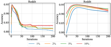
We study the over-smoothing problem by examining the convergence behavior of GraphHop on Reddit in Fig. 10. The left subfigure shows the averaged convergence curves of GraphHop on Reddit with multiple label rates. The curves drop after 5 iterations and converge at around 50 iterations. We argue that this phenomenon is due to over-smoothing of label embeddings. Generally speaking, correlations of embeddings are valid only locally. This is especially true for large-scale graphs. Adding uncorrelated information from long-distance hops tends to have negative impact. To verify this claim, we conduct experiments on a variant of GraphHop, whose label embeddings are updated in form of
| (17) |
where parameter is used to control the update speed. Eq. (17) is also known as the residual connection [31]. A large value enables the model to preserve more information from the previous iteration and slows down the smoothening speed. We report the results with in the right subfigure while keeping the other settings the same as the left subfigure. We observe more stable curves with slower performance degradation.
V-E3 Fast Convergence
We explain why convergence can be achieved by only a few iterations. This is because a small number of iterations reaches sufficiency in Corollary 1. Without loss of generality, we choose Cora and CiteSeer datasets for illustration. We calculate the number of nodes in each subset, , in Eq. (13) up to hops. The cumulative results are shown in Fig. 11. Both subfigures indicate that all nodes in the graph can be reached from labeled examples within less than 10 hops. Fast propagation of embeddings yields efficient label smoothing and fast convergence. Also, we see from Fig. 11 that higher label rates will reach sufficient iterations faster than lower label rates.
VI Comments on Related Work
Semi-supervised Learning. There is rich literature on semi-supervised learning [10], including generative models [32], the transductive support vector machine [33], entropy regularization [34], manifold learning [35] and graph-based methods [1, 36, 37, 38]. Our discussion is restricted to graph-related work. Most semi-supervised graph-based methods are built on the manifold assumption [10], where nearby nodes are close in the data manifold and, as a result, they tend to have the same labels. Early research penalizes non-smoothness along edges of a graph with the Markov random field [39], the Laplacian eigenmaps [40], spectral kernels [41], and context-based methods [42, 22]. Their main difference lies in the choice of regularization. The most popular one is the quadratic penalty term applied on nearby nodes to enforce label consistency with the data geometry. The optimization result is shown to be equivalent to LP [2]. Traditional graph methods are non-parametric, discriminative, and transductive in nature, which make them lightweight with good classification performance. To further improve the performance, methods are developed by combining graph-based regularization with other models [43, 37]. Rather than regularizing on label embeddings, this is extended to attributes [44] and even to hidden layers or auxiliary embeddings in neural networks. Manifold regularization [35] and Planetoid [45] generalize the Laplacian regularizer with a supervised classifier that imposes stronger constraints on the model learning.
Graph Neural Networks. Inspired by the recent success of convolutional neural networks (CNNs) [4, 46] on images and videos, a series of efforts have been made to generalize convolutional filters from grid-structured domains to non-Euclidean domains [47, 48, 49, 50] with theoretical support from graph signal processing [51]. The space spanned by the eigenvectors of the graph Laplacian can be regarded as a generalization of the Fourier basis. By following this idea, a deep neural architecture was formulated in [47, 48] to employ the Fourier transform as a projection onto the eigenbasis of the graph Laplacian. To overcome the expensive eigendecomposition, recurrent Chebyshev polynomials were proposed in [52] as an efficient filter for approximation. GCNs [5] further simplified it by only considering the first-order approximation in the Chebyshev polynomials. GCN has inspired quite a lot of follow-up work, e.g., [24, 53, 54, 55].
With the combination of layer-wise design and nonlinear activation, GCNs offer impressive results on the semi-supervised classification problem. Later, it was explained in [12, 6, 56, 27] that the success of GCNs is due to a lowpass filtering operation performed on node attributes. Specifically, [6, 12, 56] have shown that the powerful feature extraction ability behind the graph convolutional operation in GCNs is due to a low-pass filter applied on feature matrix to extract only smooth signals for prediction. This simplified graph convolution can be formulated as an LR classifier on the aggregated features [12]. That is, we have
| (18) |
where is the LR classifier, is the -th power of the normalized adjacency matrix, , is the classifier parameters, and is the label embeddings output as defined previously. This shed light on a simple filter design on graph feature matrix. However, in order to make a stronger low-pass filter, the power should be large, which induces an expensive cost in multiplying adjacency matrix and further be scaled to large graphs. Besides, there is no restriction on the smoothness of the predicted label embeddings.
Despite the strength of GCNs, they are limited in two aspects: 1) effective modeling of node attributes and labels jointly; 2) ease of scalability to large graphs. For the first point, unlabeled examples are not integrated into model training but only inference. Several algorithms have been proposed to tackle this deficiency. Zhang et al. [9] employed a Bayesian approach by modeling the graph structure, node attributes, and labels as a joint probability and inferring the unlabeled examples by calculating the posterior distribution. On the other hand, Qu et al. [57] used the conditional random field to embed the correlation between labeled and unlabeled examples with GCNs for feature extraction. In practice, these methods are costly and incurred by the local minimum during optimization. Another line of methods employed self-training techniques to generate pseudo-labels for unlabeled examples and used them throughout training [27, 58, 28]. However, they do not utilize the correlation between labeled and unlabeled examples effectively and often suffer from label error feedback [59]. Recently, active learning methods [60, 61] have been proposed, which directly query for labeled examples and train the model in an incremental way. They are more sophisticated in model design and more difficult to optimize.
For the second point, one main issue of GCNs is the large number of model parameters, which make their optimization very difficult for large graphs. Unlike images in computer vision or sentences in natural language processing, one graph can be large in its size while its nodes are connected without segmentation. The layer-wise convolutional operation introduces an exponential expansion of neighborhood sizes [11], which hinders GCNs from batch training. Sampling-based strategies (e.g. GraphSAGE [18] and FastGCN [29]) have been proposed to overcome this problem. They attempt to reduce the neighborhood size during aggregation. Alternatively, some methods [11, 62] directly sample one or more subgraphs and perform subgraph-level training. Recently, You et al. [30] proposed a layer-wise training algorithm for GCNs, which is called L-GCN. The idea is that, instead of training multiple GCN layers at once, the gradient update and parameters convergence are performed in a layer-wise fashion. Yet, L-GCN requires a large amount of training data (i.e., heavily supervised learning) and its performance degrades dramatically when only a few labeled examples are available in training.
VII Conclusion
A novel iterative method, called GraphHop, was proposed for transductive semi-supervised node classification on graph-structured data. It first initializes label embedding vectors through predictions based on node features. Then, based on the smooth label assumption on graphs, GraphHop propagated label embeddings iteratively to regularize the initial inference furthermore. Instead of directly replacing the embeddings by neighbor averages at each iteration, GraphHop adopts an LR classifier between iterations to align embeddings between neighbors and itself effectively. Incorporation of label initialization, label aggregation from neighbors, and label update via classifiers makes GraphHop both efficient and lightweight. Experimental results on various scales of networks demonstrate that the proposed GraphHop method offers an effective semi-supervised solution to node classification, which is especially true in extremely few labeled examples.
Appendix A Implementation of LR Classifier
We explain the implementation details of the LR classifier here. For labeled examples, the supervised loss term can be written as
| (19) |
where is the entropy loss for classification and denotes the parameters of the classifier. The missing labels for unlabeled examples prevent the direct supervision. However, we can leverage the label embedding from node itself as supervision and treat propagated embeddings as input. The explicit results are the probability predictions from the classifiers that are consistent between neighbors and node itself.
Similar ideas can be employed as regularization, so-called consistency regularization [63, 64, 65], which enforces model predictions to be consistent under any input transformations. Then, the loss term for unlabeled examples can be expressed as
| (20) |
Given the loss terms for labeled and unlabeled examples in Eqs. (19) and (20), respectively, the final loss function is a weighted sum of the two,
| (21) |
where is a hyperparameter. The LR classifier are trained in multiple epochs until convergence. Finally, new label embeddings are predicted by
| (22) |
Before training the LR classifier, we perform one additional step inspired by entropy minimization [34] and knowledge distillation [66] for supervision in Eq. (20). That is, given label embeddings, we apply a sharpening function to adjust the entropy of the label distribution. A temperature is introduced to alternate the categorical distribution, which is defined as
| (23) |
where is the input categorical distribution (i.e. label embeddings in GraphHop) and is the temperature hyperparameter. Using a higher value for produces a softer probability distribution over classes, and vice versa. By adjusting the temperature, models can decide how confidence they should believe in the current label embeddings iteration.
The sharpening operation may result in uniform label distributions by setting a large temperature. To enforce the classifier outputs low-entropy predictions on unlabeled data, we minimize the entropy [64, 34] of model prediction with an additional loss term
| (24) |
In practice, the final loss can be written as
| (25) |
where is a hyperparameter to adjust the scale of the entropy.
References
- [1] D. Zhou, O. Bousquet, T. Lal, J. Weston, and B. Schölkopf, “Learning with local and global consistency,” Advances in neural information processing systems, vol. 16, pp. 321–328, 2003.
- [2] O. Chapelle, B. Schölkopf, and A. Zien, “Label propagation and quadratic criterion,” 2006.
- [3] S. Ravi and Q. Diao, “Large scale distributed semi-supervised learning using streaming approximation,” in Artificial Intelligence and Statistics, 2016, pp. 519–528.
- [4] Y. LeCun, Y. Bengio, and G. Hinton, “Deep learning,” nature, vol. 521, no. 7553, pp. 436–444, 2015.
- [5] T. N. Kipf and M. Welling, “Semi-supervised classification with graph convolutional networks,” arXiv preprint arXiv:1609.02907, 2016.
- [6] Q. Li, X.-M. Wu, H. Liu, X. Zhang, and Z. Guan, “Label efficient semi-supervised learning via graph filtering,” in Proceedings of the IEEE Conference on Computer Vision and Pattern Recognition, 2019, pp. 9582–9591.
- [7] J. Ma, W. Tang, J. Zhu, and Q. Mei, “A flexible generative framework for graph-based semi-supervised learning,” in Advances in Neural Information Processing Systems, 2019, pp. 3281–3290.
- [8] M. Qu, Y. Bengio, and J. Tang, “Gmnn: Graph markov neural networks,” arXiv preprint arXiv:1905.06214, 2019.
- [9] Y. Zhang, S. Pal, M. Coates, and D. Ustebay, “Bayesian graph convolutional neural networks for semi-supervised classification,” in Proceedings of the AAAI Conference on Artificial Intelligence, vol. 33, 2019, pp. 5829–5836.
- [10] O. Chapelle, B. Scholkopf, and A. Zien, “Semi-supervised learning (chapelle, o. et al., eds.; 2006)[book reviews],” IEEE Transactions on Neural Networks, vol. 20, no. 3, pp. 542–542, 2009.
- [11] W.-L. Chiang, X. Liu, S. Si, Y. Li, S. Bengio, and C.-J. Hsieh, “Cluster-gcn: An efficient algorithm for training deep and large graph convolutional networks,” in Proceedings of the 25th ACM SIGKDD International Conference on Knowledge Discovery & Data Mining, 2019, pp. 257–266.
- [12] F. Wu, T. Zhang, A. H. d. Souza Jr, C. Fifty, T. Yu, and K. Q. Weinberger, “Simplifying graph convolutional networks,” arXiv preprint arXiv:1902.07153, 2019.
- [13] X. Zhu and A. B. Goldberg, “Introduction to semi-supervised learning,” Synthesis lectures on artificial intelligence and machine learning, vol. 3, no. 1, pp. 1–130, 2009.
- [14] M. Ou, P. Cui, J. Pei, Z. Zhang, and W. Zhu, “Asymmetric transitivity preserving graph embedding,” in Proceedings of the 22nd ACM SIGKDD international conference on Knowledge discovery and data mining, 2016, pp. 1105–1114.
- [15] D. P. Kingma and M. Welling, “Auto-encoding variational bayes,” arXiv preprint arXiv:1312.6114, 2013.
- [16] I. Goodfellow, J. Pouget-Abadie, M. Mirza, B. Xu, D. Warde-Farley, S. Ozair, A. Courville, and Y. Bengio, “Generative adversarial nets,” in Advances in neural information processing systems, 2014, pp. 2672–2680.
- [17] M. Zhang and Y. Chen, “Link prediction based on graph neural networks,” in Advances in Neural Information Processing Systems, 2018, pp. 5165–5175.
- [18] W. Hamilton, Z. Ying, and J. Leskovec, “Inductive representation learning on large graphs,” in Advances in neural information processing systems, 2017, pp. 1024–1034.
- [19] H. Hotelling, “Analysis of a complex of statistical variables into principal components.” Journal of educational psychology, vol. 24, no. 6, p. 417, 1933.
- [20] A. Paszke, S. Gross, S. Chintala, G. Chanan, E. Yang, Z. DeVito, Z. Lin, A. Desmaison, L. Antiga, and A. Lerer, “Automatic differentiation in pytorch,” 2017.
- [21] X. Zhu, Z. Ghahramani, and J. Lafferty, “Semi-supervised learning using gaussian fields and harmonic functions,” in Proceedings of the Twentieth International Conference on International Conference on Machine Learning, ser. ICML’03. AAAI Press, 2003, p. 912–919.
- [22] B. Perozzi, R. Al-Rfou, and S. Skiena, “Deepwalk: Online learning of social representations,” in Proceedings of the 20th ACM SIGKDD international conference on Knowledge discovery and data mining, 2014, pp. 701–710.
- [23] J. Tang, M. Qu, M. Wang, M. Zhang, J. Yan, and Q. Mei, “Line,” Proceedings of the 24th International Conference on World Wide Web - WWW ’15, 2015. [Online]. Available: http://dx.doi.org/10.1145/2736277.2741093
- [24] P. Veličković, W. Fedus, W. L. Hamilton, P. Liò, Y. Bengio, and R. D. Hjelm, “Deep graph infomax,” 2019. [Online]. Available: https://openreview.net/forum?id=rklz9iAcKQ
- [25] A. Bojchevski and S. Günnemann, “Deep gaussian embedding of graphs: Unsupervised inductive learning via ranking,” arXiv preprint arXiv:1707.03815, 2017.
- [26] P. Veličković, G. Cucurull, A. Casanova, A. Romero, P. Liò, and Y. Bengio, “Graph Attention Networks,” International Conference on Learning Representations, 2018. [Online]. Available: https://openreview.net/forum?id=rJXMpikCZ
- [27] Q. Li, Z. Han, and X.-M. Wu, “Deeper insights into graph convolutional networks for semi-supervised learning,” arXiv preprint arXiv:1801.07606, 2018.
- [28] K. Sun, Z. Zhu, and Z. Lin, “Multi-stage self-supervised learning for graph convolutional networks,” arXiv preprint arXiv:1902.11038, 2019.
- [29] J. Chen, T. Ma, and C. Xiao, “Fastgcn: fast learning with graph convolutional networks via importance sampling,” arXiv preprint arXiv:1801.10247, 2018.
- [30] Y. You, T. Chen, Z. Wang, and Y. Shen, “L2-gcn: Layer-wise and learned efficient training of graph convolutional networks,” in Proceedings of the IEEE/CVF Conference on Computer Vision and Pattern Recognition, 2020, pp. 2127–2135.
- [31] K. He, X. Zhang, S. Ren, and J. Sun, “Deep residual learning for image recognition,” in Proceedings of the IEEE conference on computer vision and pattern recognition, 2016, pp. 770–778.
- [32] D. P. Kingma, S. Mohamed, D. Jimenez Rezende, and M. Welling, “Semi-supervised learning with deep generative models,” Advances in neural information processing systems, vol. 27, pp. 3581–3589, 2014.
- [33] K. P. Bennett and A. Demiriz, “Semi-supervised support vector machines,” in Advances in Neural Information processing systems, 1999, pp. 368–374.
- [34] Y. Grandvalet and Y. Bengio, “Semi-supervised learning by entropy minimization,” in Advances in neural information processing systems, 2005, pp. 529–536.
- [35] M. Belkin, P. Niyogi, and V. Sindhwani, “Manifold regularization: A geometric framework for learning from labeled and unlabeled examples,” Journal of machine learning research, vol. 7, no. Nov, pp. 2399–2434, 2006.
- [36] D.-M. Liang and Y.-F. Li, “Lightweight label propagation for large-scale network data.” in IJCAI, 2018, pp. 3421–3427.
- [37] A. Iscen, G. Tolias, Y. Avrithis, and O. Chum, “Label propagation for deep semi-supervised learning,” in Proceedings of the IEEE conference on computer vision and pattern recognition, 2019, pp. 5070–5079.
- [38] C. Gong, T. Liu, D. Tao, K. Fu, E. Tu, and J. Yang, “Deformed graph laplacian for semisupervised learning,” IEEE transactions on neural networks and learning systems, vol. 26, no. 10, pp. 2261–2274, 2015.
- [39] X. Zhu and Z. Ghahramani, “Towards semi-supervised classification with markov random fields,” 2002.
- [40] M. Belkin and P. Niyogi, “Semi-supervised learning on riemannian manifolds,” Machine learning, vol. 56, no. 1-3, pp. 209–239, 2004.
- [41] O. Chapelle, J. Weston, and B. Schölkopf, “Cluster kernels for semi-supervised learning,” Advances in neural information processing systems, vol. 15, pp. 601–608, 2002.
- [42] A. Grover and J. Leskovec, “node2vec: Scalable feature learning for networks,” in Proceedings of the 22nd ACM SIGKDD international conference on Knowledge discovery and data mining, 2016, pp. 855–864.
- [43] P. Sen, G. Namata, M. Bilgic, L. Getoor, B. Galligher, and T. Eliassi-Rad, “Collective classification in network data,” AI magazine, vol. 29, no. 3, pp. 93–93, 2008.
- [44] J. Weston, F. Ratle, H. Mobahi, and R. Collobert, “Deep learning via semi-supervised embedding,” in Neural networks: Tricks of the trade. Springer, 2012, pp. 639–655.
- [45] Z. Yang, W. Cohen, and R. Salakhudinov, “Revisiting semi-supervised learning with graph embeddings,” in International conference on machine learning. PMLR, 2016, pp. 40–48.
- [46] Y. LeCun, Y. Bengio et al., “Convolutional networks for images, speech, and time series,” The handbook of brain theory and neural networks, vol. 3361, no. 10, p. 1995, 1995.
- [47] M. Henaff, J. Bruna, and Y. LeCun, “Deep convolutional networks on graph-structured data,” arXiv preprint arXiv:1506.05163, 2015.
- [48] J. Bruna, W. Zaremba, A. Szlam, and Y. LeCun, “Spectral networks and locally connected networks on graphs,” arXiv preprint arXiv:1312.6203, 2013.
- [49] J. Atwood and D. Towsley, “Diffusion-convolutional neural networks,” in Advances in neural information processing systems, 2016, pp. 1993–2001.
- [50] D. K. Duvenaud, D. Maclaurin, J. Iparraguirre, R. Bombarell, T. Hirzel, A. Aspuru-Guzik, and R. P. Adams, “Convolutional networks on graphs for learning molecular fingerprints,” in Advances in neural information processing systems, 2015, pp. 2224–2232.
- [51] D. I. Shuman, S. K. Narang, P. Frossard, A. Ortega, and P. Vandergheynst, “The emerging field of signal processing on graphs: Extending high-dimensional data analysis to networks and other irregular domains,” IEEE signal processing magazine, vol. 30, no. 3, pp. 83–98, 2013.
- [52] M. Defferrard, X. Bresson, and P. Vandergheynst, “Convolutional neural networks on graphs with fast localized spectral filtering,” in Advances in neural information processing systems, 2016, pp. 3844–3852.
- [53] K. Xu, W. Hu, J. Leskovec, and S. Jegelka, “How powerful are graph neural networks?” arXiv preprint arXiv:1810.00826, 2018.
- [54] I. Spinelli, S. Scardapane, and A. Uncini, “Adaptive propagation graph convolutional network,” arXiv preprint arXiv:2002.10306, 2020.
- [55] Z. Wu, S. Pan, F. Chen, G. Long, C. Zhang, and S. Y. Philip, “A comprehensive survey on graph neural networks,” IEEE Transactions on Neural Networks and Learning Systems, 2020.
- [56] H. NT and T. Maehara, “Revisiting graph neural networks: All we have is low-pass filters,” arXiv preprint arXiv:1905.09550, 2019.
- [57] M. Qu, Y. Bengio, and J. Tang, “Gmnn: Graph markov neural networks,” 2020.
- [58] Y. You, T. Chen, Z. Wang, and Y. Shen, “When does self-supervision help graph convolutional networks?” arXiv preprint arXiv:2006.09136, 2020.
- [59] D.-H. Lee, “Pseudo-label: The simple and efficient semi-supervised learning method for deep neural networks,” in Workshop on challenges in representation learning, ICML, vol. 3, no. 2, 2013.
- [60] Y. Li, J. Yin, and L. Chen, “Seal: Semisupervised adversarial active learning on attributed graphs,” IEEE Transactions on Neural Networks and Learning Systems, 2020.
- [61] H. Yu, X. Yang, S. Zheng, and C. Sun, “Active learning from imbalanced data: A solution of online weighted extreme learning machine,” IEEE Transactions on Neural Networks and Learning Systems, vol. 30, no. 4, pp. 1088–1103, 2018.
- [62] H. Zeng, H. Zhou, A. Srivastava, R. Kannan, and V. Prasanna, “Graphsaint: Graph sampling based inductive learning method,” arXiv preprint arXiv:1907.04931, 2019.
- [63] A. Tarvainen and H. Valpola, “Mean teachers are better role models: Weight-averaged consistency targets improve semi-supervised deep learning results,” in Advances in neural information processing systems, 2017, pp. 1195–1204.
- [64] D. Berthelot, N. Carlini, I. Goodfellow, N. Papernot, A. Oliver, and C. A. Raffel, “Mixmatch: A holistic approach to semi-supervised learning,” in Advances in Neural Information Processing Systems, 2019, pp. 5049–5059.
- [65] T. Miyato, S. Maeda, M. Koyama, and S. Ishii, “Virtual adversarial training: A regularization method for supervised and semi-supervised learning,” IEEE Transactions on Pattern Analysis and Machine Intelligence, vol. 41, no. 8, pp. 1979–1993, 2019.
- [66] G. Hinton, O. Vinyals, and J. Dean, “Distilling the knowledge in a neural network,” 2015.