This paper was converted on www.awesomepapers.org from LaTeX by an anonymous user.
Want to know more? Visit the Converter page.

Graph Topic Modeling for Documents with Spatial or Covariate Dependencies

Yeo Jin Jung
Department of Statistics, The University of Chicago
and
Claire Donnat
Department of Statistics, The University of Chicago
Abstract

We address the challenge of incorporating document-level metadata into topic modeling to improve topic mixture estimation. To overcome the computational complexity and lack of theoretical guarantees in existing Bayesian methods, we extend probabilistic latent semantic indexing (pLSI), a frequentist framework for topic modeling, by incorporating document-level covariates or known similarities between documents through a graph formalism. Modeling documents as nodes and edges denoting similarities, we propose a new estimator based on a fast graph-regularized iterative singular value decomposition (SVD) that encourages similar documents to share similar topic mixture proportions. We characterize the estimation error of our proposed method by deriving high-probability bounds and develop a specialized cross-validation method to optimize our regularization parameters. We validate our model through comprehensive experiments on synthetic datasets and three real-world corpora, demonstrating improved performance and faster inference compared to existing Bayesian methods.


Keywords: graph cross validation, graph regularization, latent dirichlet allocation, total variation penalty

1 Introduction

Consider a corpus of nn documents, each composed of words (or more generally, terms) from a vocabulary of size pp. This corpus can be represented by a document-term matrix Dn×pD\in\mathbb{N}^{n\times p}, where each entry DijD_{ij} denotes the number of times term jj appears in document ii. The objective of topic modeling is to retrieve low-dimensional representations of the data by representing each document as a mixture of latent topics, defined as distributions over term frequencies.

In this setting, each document DipD_{i\cdot}\in\mathbb{R}^{p} is usually assumed to be sampled from a multinomial distribution with an associated probability vector MipM_{i\cdot}\in\mathbb{R}^{p} that can be decomposed as a mixture of KK topics. In other words, letting NiN_{i} denote the length of document ii:

i=1,,n,DiMultinomial(Ni,Mi),with Mi=k=1KWikAk\forall i=1,\cdots,n,\qquad D_{i\cdot}\sim\text{Multinomial}(N_{i},M_{i\cdot}),\qquad\text{with }M_{i\cdot}=\sum_{k=1}^{K}W_{ik}A_{k\cdot} (1)

In the previous equation, WikW_{ik} corresponds to the proportion of topic kk in document ii, and the vector WiW_{i\cdot} provides a low-dimensional representation of document ii in terms of its topic composition. Each entry AkjA_{kj} of the vector AkpA_{k\cdot}\in\mathbb{R}^{p} corresponds to the expected frequency of word jj in topic kk. Since document lengths {Ni}i=1n\{N_{i}\}_{i=1}^{n} are usually treated as nuisance variables, most topic modeling approaches work in fact directly with the word frequency matrix X=diag({1Ni}i=1n)DX=\text{diag}(\{\frac{1}{N_{i}}\}_{i=1\cdots n})D, which can be written in a “signal + noise” form as:

X=M+Z=WA+Z.X=M+Z=WA+Z. (2)

Here, Mn×pM\in\mathbb{R}^{n\times p} is the true signal whose entry MijM_{ij} denotes the expected frequency of word ii in document jj, while Z=XMZ=X-M denotes some centered multinomial noise. The objective of topic modeling is thus to estimate WW and AA from XX.

Originally developed to reduce document representations to low-dimensional latent semantic spaces, topic modeling has been successfully deployed for the analysis of count data in a number of applications, ranging from image processing (Tu et al. 2016, Zheng et al. 2015) and image annotation(Feng & Lapata 2010, Shao et al. 2009), to biochemistry (Reder et al. 2021), genetics (Dey et al. 2017, Kho et al. 2017, Liu et al. 2016, Yang et al. 2019), and microbiome studies (Sankaran & Holmes 2019, Symul et al. 2023).

A notable extension of topic modeling occurs when additional document-level data is available. Although original topic modeling approaches rely solely on the analysis of the empirical frequency matrix XX, this additional information has the potential to significantly improve the estimation of the word-topic matrix AA and the document-topic mixture matrix WW, particularly in difficult inference settings, such as when the number of words per document is small. Examples include:

  1. 1.

    Analyzing tumor microenvironments: In this context, slices of tumor samples are partitioned into smaller regions known as tumor microenvironments, where the frequency of specific immune cell types is recorded (Chen et al. 2020). Here, documents correspond to microenvironments, and words to cell types. The objective is to identify communities of co-abundant cells (topics), taken here as proxies for tumor-immune cell interactions and potential predictors of patient outcomes. In this setting, we assume that neighboring microenvironments share similar topic proportions. Since these microenvironments are inherently small, leveraging the spatial smoothness of the mixture matrix WW can significantly improve inference (Chen et al. 2020). We develop this example in further detail in Section 4.1.

  2. 2.

    Microbiome studies: Topic models have also been proven to be extremely useful in microbiome analysis (Sankaran & Holmes 2019, Symul et al. 2023). In this setting, the data consists of a microbiome count matrix recording the amount of different types of bacteria found in each sample. In this case, microbiome samples are identified to documents, with bacteria playing the roles of the vocabulary, and the goal becomes to identify communities of co-abundant bacteria (Sankaran & Holmes 2019). When additional covariate information is available (such as age, gender, and other demographic details), we can expect similar samples (documents) to exhibit similar community compositions (topic proportions).

  3. 3.

    The analysis of short documents, such as a collection of scientific abstracts or recipes: In this case, while recipes might be short, information on the origin of the recipe can help determine the topics and mixture matrix more accurately by leveraging the assumption that recipes of neighboring countries will typically share similar topic proportions. We elaborate on this example in greater detail in Section 4.3.

Prior works. Previous attempts to incorporate metadata in topic estimation have focused on the Bayesian extensions of latent Dirichlet allocation (LDA) model of Blei et al. (2001). By and large, these methods typically incorporate the metadata—often in the form of a covariate matrix—within a prior distribution (Blei & Lafferty 2006a, b, Roberts et al. 2014, Mcauliffe & Blei 2007). However, these models (a) are difficult to adapt to different types of covariates or information encoded as a graph, and (b) typically lack theoretical guarantees. Recent work by Chen et al. (2020) proposes extending LDA to analyze documents with known similarities by smoothing the topic proportion hyperparameters along the edges of the graph. However, this method does not empirically yield spatially smooth structures (see Sections  3.4 and  4), and significantly increases the algorithm’s running time.

In the frequentist realm, probabilistic latent semantic indexing (pLSI) has gained renewed interest over the past five years. Similar to LDA, it effectively models documents as bags of words but differs by treating matrices AA and WW as fixed parameters. In particular, new work by Ke & Wang (2017) and Klopp et al. (2021) suggest procedures to reliably estimate the topic matrix AA and mixture matrix WW, characterizing consistency and efficiency through high-probability error bounds Although recent work has begun investigating the use of structures in pLSI-based topic models, most approaches have limited this to considering various versions of sparsity (Bing et al. 2020, Wu et al. 2023) or weak sparsity (Tran et al. 2023) for the topic matrix AA. To the best of our knowledge, no pLSI approach has yet been proposed that effectively leverages similarities between documents nor characterizes the consistency of these estimators.

Contributions

In this paper, we propose the first pLSI method that can be made amenable to the inclusion of additional information on the similarity between documents, as encoded by a known graph. More specifically:

  • a.

    We propose a scalable algorithm based on a graph-aligned singular decomposition of the empirical frequency matrix XX to provide estimates of WW and AA (Section 2). Additionally, we develop a new cross-validation procedure for our graph-based penalty that allows us to choose the optimal regularization parameter adaptively (Section A of the Appendix).

  • b.

    We prove the benefits of the graph alignment procedure by deriving high probability upper bounds for both WW and AA in Section 3, which we verify through extensive simulations in Section 3.4.

  • c.

    Finally, we showcase the advantage of our method over LDA-based methods and non-structured pLSI techniques on three real-world datasets: two spatial transcriptomics examples and a recipe dataset in Section 4.

Notations

Throughout this paper, we use the following notations. For any t+t\in\mathbb{Z}_{+}, [t][t] denotes the set {1,2,,t}\{1,2,...,t\}. For any a,ba,b\in\mathbb{R}, we write ab=max(a,b)a\vee b=\max(a,b) and ab=min(a,b){a\wedge b=\min(a,b)}. We use 𝟏dd\mathbf{1}_{d}\in\mathbb{R}^{d} to denote the vector with all entries equal to 1 and 𝐞kd\mathbf{e}_{k}\in\mathbb{R}^{d} to denote the vector with kthk^{th} element set to 1 and 0 otherwise. For any vector uu, its 2\ell_{2}, 1\ell_{1} and 0\ell_{0} norms are defined respectively as u2=iui2\|u\|_{2}=\sqrt{\sum_{i}u_{i}^{2}}, u1=i|ui|\|u\|_{1}=\sum_{i}|u_{i}|, and u0=i𝟏{ui0}\|u\|_{0}=\sum_{i}\mathbf{1}\{u_{i}\neq 0\}. Let ImI_{m} denote the m×mm\times m identity matrix. For any matrix A=(aij)n×p{A=(a_{ij})\in\mathbb{R}^{n\times p}}, A(i,j)A(i,j) denote the (i,j)(i,j)-entry of AA, AiA_{i\cdot} and AjA_{\cdot j} denote the ithi^{\text{th}} row and jthj^{th} column of AA respectively. Throughout this paper, λi(A)\lambda_{i}(A) stands for the ithi^{th} largest singular value of the matrix AA with λmax(A)=λ1(A){\lambda_{\max}(A)=\lambda_{1}(A)}, λmin(A)=λprank(A)(A){\lambda_{\min}(A)=\lambda_{p\wedge\text{rank}(A)}(A)}. We also denote as UK(A)U_{K}(A) and VK(A)V_{K}(A) the left and right singular matrix from the rank-KK SVD of AA. The Frobenius, entry-wise 1\ell_{1} norm and the operator norms of AA are denoted as AF=i,jaij2\left\|A\right\|_{F}=\sqrt{\sum_{i,j}a_{ij}^{2}}, A11=i,j|aij|\lVert A\rVert_{11}=\sum_{i,j}|a_{ij}|, and Aop=λ1(A){\left\|A\right\|_{op}=\lambda_{1}(A)}, respectively. The 21\ell_{21} norm is denoted as A21=iAi2\big{\|}A\big{\|}_{21}=\sum_{i}\|A_{i\cdot}\|_{2}. For any positive semi-definite matrix AA, A1/2A^{1/2} denotes its principal square root that is positive semi-definite and satisfies A1/2A1/2=AA^{1/2}A^{1/2}=A. The trace inner product of two matrices A,Bn×pA,B\in\mathbb{R}^{n\times p} is denoted by A,B=𝖳𝗋(AB)\langle A,B\rangle=\mathop{\sf Tr}(A^{\top}B). AA^{\dagger} denotes the pseudo-inverse of the matrix AA and PAP_{A} denotes the projection matrix onto the subspace spanned by columns of AA.

2 Graph-Aligned pLSI

In this section, we introduce graph-aligned pLSI (GpLSI), an extension of the standard pLSI framework that leverages known similarities between documents to improve inference in topic modeling using a graph formalism. We begin by introducing a set of additional notations and model assumptions, before introducing the algorithm in Section 2.3.

2.1 Assumptions

Let 𝒢=(𝒟,)\mathcal{G}=(\mathcal{D},\mathcal{E}) denote an undirected graph induced by a known adjacency matrix on the nn documents in the corpus. The documents are represented as nodes 𝒟\mathcal{D}, and \mathcal{E} denotes the edge set of size ||=m\lvert\mathcal{E}\rvert=m. Throughout this paper, for simplicity, we will assume that 𝒢\mathcal{G} is binary, but our approach—as discussed in Section 2.3—can be in principle extended to weighted graphs. We denote the graph’s incidence matrix as Γm×n\Gamma\in\mathbb{R}^{m\times n} where, for any edge e=(i,j),i<je=(i,j),i<j between nodes ii and jj in the graph, Γei=1\Gamma_{ei}=1, Γej=1\Gamma_{ej}=-1 and Γek=0\Gamma_{ek}=0 for any ki,j.k\neq i,j. It is easy to show that the Laplacian of the graph can be expressed in terms of the incidence matrix as L=ΓΓL=\Gamma^{\top}\Gamma (Hütter & Rigollet 2016). Let Γ\Gamma^{\dagger} be the pseudo-inverse of Γ\Gamma, and denote by 𝐬i,i=1m\mathbf{s}_{i},i=1\cdots m its columns, so that Γ=[𝐬1,,𝐬m]\Gamma^{\dagger}=[\mathbf{s}_{1},\cdots,\mathbf{s}_{m}]. We also define the inverse scaling factor of the incidence matrix Γ\Gamma (Hütter & Rigollet 2016), a quantity necessary for assessing the performance of GpLSI:

ρ(Γ)maxl[m]𝐬l2\rho(\Gamma)\coloneqq\max_{l\in[m]}\|{\mathbf{s}_{l}}\|_{2} (3)

We focus on the estimation of the topic mixture matrix under the assumption that neighboring documents have similar topic mixture proportions: WiWjW_{i\cdot}\approx W_{j\cdot} if iji\sim j. This implies that the rows of WW are assumed to be smooth with respect to the graph 𝒢\mathcal{G}. Noting that the difference of mixture proportions between neighboring nodes ii and jj (e=(i,j)e=(i,j)\in\mathcal{E}) can be written as (ΓW)d=WiWj(\Gamma W)_{d\cdot}=W_{i\cdot}-W_{j\cdot}, this smoothness assumption effectively implies sparsity on the rows of the matrix ΓW\Gamma W.

Assumption 1 (Graph-Aligned mixture matrix).

The support (i.e, the number of non-zero rows) of the difference matrix ΓW=(WiWj)(i,j)\Gamma W=\left(W_{i\cdot}-W_{j\cdot}\right)_{(i,j)\in\mathcal{E}} is small:

|supp(ΓW)|s,|\text{supp}(\Gamma W)|\leq s, (4)

where s||,n.s\ll|\mathcal{E}|,n.

The previous assumption is akin to assuming that the underlying mixture matrix WW is piecewise-continuous with respect to the graph 𝒢\mathcal{G}, or more generally, that it can be well approximated by a piecewise-continuous function.

Our setting is not limited to connected document graphs. Denote n𝒞n_{\mathcal{C}} the number of connected subgraphs of 𝒢\mathcal{G} and n𝒞ln_{\mathcal{C}_{l}} the number of nodes in the lthl^{th} connected subgraph. Let n𝒞minn_{\mathcal{C}_{\min}} be the size of the smallest connected component:

n𝒞min=minl[n𝒞]n𝒞ln_{\mathcal{C}_{\min}}=\min_{l\in[n_{\mathcal{C}}]}n_{\mathcal{C}_{l}} (5)

The error bound of our estimators will depend on both n𝒞n_{\mathcal{C}} and n𝒞minn_{\mathcal{C}_{\min}}. In the rest of this paper, we will assume that all connected components have roughly the same size: n𝒞1n𝒞n𝒞n_{\mathcal{C}_{1}}\asymp\dots\asymp n_{\mathcal{C}_{n_{\mathcal{C}}}}.

Assumption 2 (Anchor document).

For each topic k=1,,K,k=1,\dots,K, there exists at least one document ii (called an anchor document) such that Wik=1W_{ik}=1 and Wik=0W_{ik^{{}^{\prime}}}=0 for all kkk^{{}^{\prime}}\not=k.

Remark 1.

Assumption 2 is standard in the topic modeling community, as it is a sufficient condition for the identifiability of the topic and mixture matrices AA and WW (Donoho & Stodden 2003). Beyond identifiability, we contend that the “anchor document” assumption functions not only as a sufficient condition for identifiability but also as a necessary condition for interpretability: Topics are interpretable only when associated with archetypes—that is, “extreme“ representations (in our case, anchor documents)—that illustrate the topic more expressively.

Assumption 3 (Equal Document Sizes).

In this paper, for ease of presentation, we will also assume that the documents have equal sizes: N1==Nn=NN_{1}=\dots=N_{n}=N. More generally, our results also hold if we assume that the document lengths satisfy maxi[n]NiCmini[n]Ni\max_{i\in[n]}N_{i}\leq C^{*}\min_{i\in[n]}N_{i} (N1NnN_{1}\asymp\dots\asymp N_{n}), in which case N=1ni=1nNiN=\frac{1}{n}\sum_{i=1}^{n}N_{i} denotes the average document length.

Assumption 4 (Condition number of MM and WW).

There exist two constants c,c>0c,c^{*}>0 such that

λK(M)cλ1(W)andmax{κ(M),κ(W)}c.\lambda_{K}(M)\geq c\lambda_{1}(W)\quad\text{and}\quad\max\left\{\kappa(M),\kappa(W)\right\}\leq c^{*}.
Assumption 5 (Assumption on the minimum word frequency).

We assume that the expected word frequencies hjh_{j} defined as: j[p],hj=k=1KAkj\forall j\in[p],h_{j}=\sum_{k=1}^{K}A_{kj} are bounded below by:

minj[p]hjcminlog(n)N\min_{j\in[p]}h_{j}\geq c_{\min}\frac{\log(n)}{N}

where cminc_{\min} is a constant that does not depend on parameters n,p,Nn,p,N or KK.

Remark 2.

Assumption 5 is a relatively strong assumption that essentially restricts the scope of this paper’s analysis to small vocabulary sizes (thereafter referred to as the “low-pp” regime). Indeed, since j=1pk=1KAkj=K\sum_{j=1}^{p}\sum_{k=1}^{K}A_{kj}=K, under Assumption 5, it immediately follows that:

pcminlog(n)NKpKNlog(n)cminpc_{\min}\frac{\log(n)}{N}\leq K\implies p\leq\frac{KN}{\log(n)c_{\min}}

This assumption might not reflect the large vocabulary sizes found in many practical problems, where we could expect pp to grow with nn. A solution to this potential limitation is to assume weak sparsity on the matrix AA and to threshold away rare terms using the thresholding procedure proposed in Tran et al. (2023), selecting a subset JJ of words with large enough frequency. In this case, the rest of our analysis should follow, replacing simply the data matrix XX by its subset, XJ.X_{\cdot J}.

2.2 Estimation procedure: pLSI

Since the smoothness assumption (Assumption 1) pertains to the rows of the document-topic mixture matrix WW, we build on the pLSI algorithm developed by Klopp et al. (2021). In this subsection, we provide a brief overview of their method.

When we assume we directly observe the true expected frequency matrix MM defined in Equation (2), Klopp et al. (2021) propose a fast and simple procedure to recover the mixture matrix WW. Specifically, let Un×KU\in\mathbb{R}^{n\times K} and Vp×KV\in\mathbb{R}^{p\times K} be the left and right singular vectors obtained from the singular value decomposition (SVD) of the true signal Mn×pM\in\mathbb{R}^{n\times p}, so that M=UΛVTM=U\Lambda V^{T}. A critical insight from their work is that UU can be decomposed as:

U=WH,U=WH, (6)

where HH is a full-rank, K×KK\times K-dimensional matrix. From this decomposition, it follows that the rows of UU, which can be viewed as KK-dimensional embeddings of the documents, lie on the KK-dimensional simplex ΔK1\Delta_{K-1}. The simplex’s vertices, represented by the rows of HH, correspond to the anchor documents (Assumption 2). Thus, identifying these vertices through any standard vertex-finding algorithm applied to the rows of UU will enable the estimation of WW. The procedure of Klopp et al. (2021) can be summarized as follows:

Step 1:

Compute the singular value decomposition (SVD) of the matrix MM, reduced to rank KK, to obtain: M=UΛVTM=U\Lambda V^{T}.

Step 2: Vertex-Hunting Step:

Apply the successive projection algorithm (SPA) (Araújo et al. 2001) (a vertex-hunting algorithm) on the rows of UU. This algorithm returns the indices of the selected “anchor documents,” J[n]J\subseteq[n] with |J|=K|J|=K. Define H^=UJ\widehat{H}=U_{J\cdot}, where each row corresponds to one of the KK vertices of the simplex ΔK1\Delta_{K-1}.

Step 3: Recovery of WW:

WW can simply be recovered from UU and H^\widehat{H} as

W^=UH^1.\widehat{W}={U}\widehat{H}^{-1}. (7)
Step 4: Recovery of AA:

Finally, AA can subsequently be estimated as A^=H^ΛV.\widehat{A}=\widehat{H}\Lambda V^{\top}.

In the noisy setting, the procedure is adapted by plugging the observed frequency XX instead of MM in Step 1 and getting estimates of the singular vectors: X=U^Λ^V^X=\widehat{U}\widehat{\Lambda}\widehat{V}^{\top}. Under a similar set of assumptions as ours (Assumptions 2-4), Theorem 1 of (Klopp et al. 2021) states that the error of W^\widehat{W} is such that: minP𝒫W^WPFC0Knlog(n+p)/N\min_{P\in\mathcal{P}}\|\widehat{W}-WP\|_{F}\leq{\rm C_{0}}K\sqrt{n\log(n+p)/N}, where 𝒫\mathcal{P} denotes the set of all permutation matrices. Their analysis provides one of the best error bounds on the estimation of the topic mixture matrix WW for pLSI.

However, this approach has two key limitations. First, the consistency of their estimator relies on having a sufficiently large number of words per document, NN. In particular, a necessary condition for the aforementioned results to hold is that NCK5log(n+p)N\geq CK^{5}\log(n+p). The authors establish minimax error bounds, showing that the rate of any estimator’s error for WW is bounded below by a term on the order of O(n/N)O(\sqrt{n/N}) (Theorem 3, Klopp et al. (2021)). In other words, the accurate estimation of WW requires that each document contains enough words. In many practical scenarios—such as the tumor microenvironment example mentioned earlier—this condition may not hold. However, we might still have access to additional information indicating that certain documents are more similar to one another.

Second, the method is relatively rigid and does not easily accommodate additional structural information, such as document-level similarities. Indeed, this method does not rely on a convex optimization formulation to which we could simply add a regularization term, and the vertex-hunting algorithm does not readily incorporate metadata of the documents.

2.3 Estimation procedure: GpLSI

Theoretical insights from Klopp et al. (2021) help explain why topic modeling deteriorates in low-NN regimes. When the number of words per document is too small, the observed frequency matrix XX can be viewed as a highly noisy approximation of MM, causing the estimated singular vectors U^\widehat{U} to deviate significantly from the true underlying point cloud UU. To mitigate this issue, Klopp et al. (2021) suggest a preconditioning step that improves the estimation of the singular vectors in noisy settings.

In this paper, we take a different approach by exploiting the graph structure associated with the documents to reduce the noise in XX. Rather than preconditioning the empirical frequency matrix, we propose an additional denoising step that leverages the graph structure to produce more accurate estimates of UU, VV, and Λ\Lambda. Specifically, we modify the SVD of XX in Step 1 and estimation of topic matrix AA in Step 4 described in Section 2.2.

Step 1: Iterative Graph-Aligned SVD of XX:

We replace Step 1 of Section 2.2 with a graph-aligned SVD of the empirical word-frequency matrix XX. More specifically, in the graph-aligned setting, we assume that the underlying frequency matrix MM belongs to the set:

(n,p,K,s)={M=UΛVn×p,rank(M)=K:Un×K,Vp×K,Λ=diag(λ1,λ2,,λK),|supp(ΓU)|s,λK>0}.\begin{split}\mathcal{F}(n,p,K,s)=\{&M=U\Lambda V^{\top}\in\mathbb{R}^{n\times p},\ \mathrm{rank}(M)=K:\\ &U\in\mathbb{R}^{n\times K},V\in\mathbb{R}^{p\times K},\Lambda=\mathrm{diag}(\lambda_{1},\lambda_{2},\cdots,\lambda_{K}),\\ &|\mathrm{supp}(\Gamma U)|\leq s,\lambda_{K}>0\}.\end{split} (8)

Throughout the paper, we shall allow s,p,N,s,p,N, and nn to vary. We will assume the number of topics KK to be fixed.

Step 2, 3

Same as Step 2,3 in Section 2.2.

Step 4: Recovery of AA:

AA can subsequently be estimated by solving a constrained regression problem of XX on W^\widehat{W}:

A^=argminAK×pXW^AF2 such that k[K],j=1pAkj=1,Akj0\begin{split}\widehat{A}&=\text{argmin}_{A\in\mathbb{R}^{K\times p}}\|X-\widehat{W}A\|_{F}^{2}\\ &\text{ such that }\forall k\in[K],\ \sum_{j=1}^{p}A_{kj}=1,\ A_{kj}\geq 0\end{split} (9)
Iterative Graph-Aligned SVD.

We propose a power iteration method for Step 1 that iteratively updates the left and right singular vectors while constraining the left singular vector to be aligned with the graph (Algorithm 1). A similar approach has already been studied under Gaussian noise in Yang et al. (2016) where sparsity constraints were imposed on the left and right singular vectors.

Drawing inspiration from Yang et al. (2016) and adapting this method to the multinomial noise setting, Algorithm 1 iterates between three steps. The first consists of denoising the left singular subspace by leveraging the graph-smoothness assumption (Assumption 1). At iteration tt, we solve:

U¯t=argminUn×KUXV^t1F2+ρ^tΓU21\bar{U}^{t}=\arg\min_{U\in\mathbb{R}^{n\times K}}\lVert U-X\widehat{V}^{t-1}\rVert_{F}^{2}+{\hat{\rho}}^{t}\lVert\Gamma U\rVert_{21} (10)

Here, U¯t\bar{U}^{t} is a denoised version of the projection XV^t1X\widehat{V}^{t-1} that leverages the graph structure to yield an estimate closer to the true UU. We then take a rank-KK SVD of U¯t\bar{U}^{t} to extract U^t\widehat{U}^{t} (an estimate of UU) with orthogonal columns.

Algorithm 1 Two-way Iterative Graph-Aligned SVD
1:Input: Observation XX, initial matrix V^0\widehat{V}^{0}, incidence matrix Γ\Gamma, number of topics KK, tolerance level ϵ\epsilon
2:Output: Denoised singular vectors U^\widehat{U}, V^\widehat{V}
3:repeat
4:     1. Graph denoising of UU : U¯t=argminUn×KUXV^t1F2+ρ^tΓU21\bar{U}^{t}=\arg\min_{U\in\mathbb{R}^{n\times K}}\lVert U-X\widehat{V}^{t-1}\rVert_{F}^{2}+\hat{\rho}^{t}\lVert\Gamma U\rVert_{21}
5:     2. SVD of U¯t\bar{U}^{t}: U^tLeft Singular Vectors in SVDK(U¯t)\widehat{U}^{t}\leftarrow\text{Left Singular Vectors in }SVD_{K}(\bar{U}^{t})
6:     3. SVD of V^t\widehat{V}^{t}: V^tLeft Singular Vectors in SVDK(XU^t)\widehat{V}^{t}\leftarrow\text{Left Singular Vectors in }SVD_{K}(X^{\top}\widehat{U}^{t})
7:     4. Calculate the score s=P^utXP^vtP^ut1XP^vt1s=\lVert\widehat{P}_{u}^{t}X\widehat{P}_{v}^{t}-\widehat{P}_{u}^{t-1}X\widehat{P}_{v}^{t-1}\rVert, P^u=U^t(U^t)\widehat{P}_{u}=\widehat{U}^{t}(\widehat{U}^{t})^{\top}, P^v=V^t(V^t)\widehat{P}_{v}=\widehat{V}^{t}(\widehat{V}^{t})^{\top}
8:until s<ϵs<\epsilon

Finally, we update V^t\widehat{V}^{t}. Since we are not assuming any particular structure on the right singular subspace, we simply apply a rank-KK SVD on the projection XU^tX^{\top}\widehat{U}^{t}. Denoting the projections onto the columns of the estimates as Put=U^t(U^t)P_{u}^{t}=\widehat{U}^{t}(\widehat{U}^{t})^{\top} and Pvt=V^t(V^t)P_{v}^{t}=\widehat{V}^{t}(\widehat{V}^{t})^{\top}, we iterate the procedure until PutXPvtPut1XPvt1Fϵ\|P_{u}^{t}XP_{v}^{t}-P_{u}^{t-1}XP_{v}^{t-1}\|_{F}\leq\epsilon for a fixed threshold ϵ\epsilon.

Denoting the final estimates after tmaxt_{\max} iterations as U^,V^\widehat{U},\widehat{V}, these estimates can then be plugged into Steps 2-4 to estimate WW and AA. The improved estimation of U^,V^\widehat{U},\widehat{V} can be shown to translate into a more accurate estimation of the matrices WW and AA (Theorems 3 and 4 presented in the next section).

Although our theoretical results depend on choosing an appropriate level of regularization ρ^t\hat{\rho}^{t}, the theoretical value of ρ^t\hat{\rho}^{t} depends on unknown graph quantities. In practice, therefore, the optimal ρ^t\hat{\rho}^{t} must be chosen in each iteration using cross-validation. We devise a novel graph cross-validation method which effectively finds the optimal graph regularization parameter by partitioning nodes into folds using a minimum spanning tree. We defer the detailed procedure to Section A of the Appendix.

Remark 3.

While in the rest of the paper, we typically assume that the graph is binary, our method is in principle generalizable to a weighted graph 𝒢=(𝒟,𝒲)\mathcal{G}=(\mathcal{D},\mathcal{W}) where 𝒲\mathcal{W} represents the weighted edge set. In this case, we denote weighted incidence matrix as Γ~=TΓ\tilde{\Gamma}=\mathrm{T}\Gamma where Tm×m\mathrm{T}\in\mathbb{R}^{m\times m} is a diagonal matrix with entry tddt_{dd} corresponding to the weight of the dthd^{th} edge. We note that scaling Γ\Gamma with T\mathrm{T} does not change the projection onto the row space of Γ\Gamma, thus preserving our theoretical results. Without loss of generality, we work with an unweighted incidence matrix Γ\Gamma.

Remark 4.

The penalty ΓU21\|\Gamma U\|_{21} is known as the total-variation penalty in the computer vision literature. As noted in Hütter & Rigollet (2016), this type of penalty is usually a good idea whenever the rows of WW take similar values, or may at least be well approximated by piecewise-constant functions. In the implementation of our algorithm, we employ the solver of developed by Sun et al. (2021), as it is the most efficient algorithm available for this type of problem.

Initialization.

The success of the procedure heavily depends on having access to good initial values for VV. Since, as highlighted in Remark 2, this manuscript assumes a “low-pp” regime, we propose to simply take the rank-KK eigendecomposition of the matrix XXnND^0X^{\top}X-\frac{n}{N}\hat{D}_{0} to obtain an initial estimate V^0\widehat{V}^{0}:

V^0=UK(XXnND^0)\widehat{V}^{0}=U_{K}({X^{\top}X}-\frac{n}{N}\widehat{D}_{0}) (11)

where D^0\widehat{D}_{0} is a diagonal matrix where each entry is defined as: (D^0)jj=1ni=1nXij,(\widehat{D}_{0})_{jj}=\frac{1}{n}\sum_{i=1}^{n}X_{ij}, and where UK(XXnND^0)U_{K}({X^{\top}X}-\frac{n}{N}\hat{D}_{0}) denotes the matrix of KK leading eigenvectors of XXnND^0{X^{\top}X-\frac{n}{N}\widehat{D}_{0}}.

Theorem 1.

Suppose max(K,p)n\max(K,p)\leq n and Kp\sqrt{K}\leq p. Under Assumptions 1 to 5, the eigenvectors of the matrix XXnND^0{X^{\top}X}-\frac{n}{N}\hat{D}_{0} provide a reasonable approximation to the right singular vectors, in that with probability at least 1o(n1)1-o(n^{-1}):

sinΘ(V,V^0)opsinΘ(V,V^0)FCλK(M)2Knlog(n)NCK2log(n)nN\begin{split}\|\sin\Theta(V,\widehat{V}^{0})\|_{op}\leq\|\sin\Theta(V,\widehat{V}^{0})\|_{F}\leq\frac{C}{\lambda_{K}(M)^{2}}K\sqrt{\frac{n\log(n)}{N}}&\leq C^{*}K^{2}\sqrt{\frac{\log(n)}{nN}}\end{split}

for some constants CC and C>0C^{*}>0.

The proof of the theorem is provided in Section B of the Appendix.

3 Theoretical results

In this section, we provide high-probability bounds on the Frobenius norm of the errors for W^\widehat{W} and A^\widehat{A}. We begin by characterizing the effect of the denoising on the estimates of the singular values of XX, before showing how the improved estimation of the singular vectors translates into improved error bounds for both WW and AA.

3.1 Denoising the singular vectors

The improvement in the estimation of the singular vectors induced by our iterative denoising procedure is characterized in the following theorem.

Theorem 2.

Let Assumption 1 to 5 hold. Assume max(K,p)n\max(K,p)\leq n and Kp\sqrt{K}\leq p. Denote U^,V^\widehat{U},\widehat{V} as outputs of Algorithm 1 after tmaxt_{\max} iterations. If NN satisfies

Ncmin(K4log(n)n(n𝒞+ρ2(Γ)sλmax(Γ))log(n)n𝒞min),N\geq c^{*}_{\min}\left(K^{4}\frac{\log(n)}{n}\left(n_{\mathcal{C}}+\rho^{2}(\Gamma)s\lambda_{\max}(\Gamma)\right)\vee\frac{\log(n)}{n_{\mathcal{C}_{\min}}}\right), (12)

there exists a constant C0>0C_{0}>0 such that with probability at least 1o(n1)1-o(n^{-1}),

max{infO𝕆KU^UOF,infO𝕆KV^VOF}C0Klog(n)nN(n𝒞+ρ(Γ)sλmax(Γ))\max\{\inf_{O\in\mathbb{O}_{K}}\|\widehat{U}-UO\|_{F},\inf_{O\in\mathbb{O}_{K}}\|\widehat{V}-VO\|_{F}\}\leq C_{0}K\sqrt{\frac{\log(n)}{nN}}\left(\sqrt{n_{\mathcal{C}}}+\rho(\Gamma)\sqrt{s\lambda_{\max}(\Gamma)}\right) (13)

The proof of this result is provided in Section C of the Appendix.

Remark 5.

This result is to be compared against the rates of the estimates obtained without any regularization. In this case, the results of Klopp et al. (2021) show that with probability at least 1o((n+p)1)1-o((n+p)^{-1}), the error in (13) is of the order of O(Klog(n)/N)O(K\sqrt{\log(n)/{N}}). Both rates thus share a factor Klog(n)/NK\sqrt{\log(n)/N}. However, the spatial regularization in our setting allows us to introduce an additional factor of the order of 1n(n𝒞+ρ(Γ)sλmax(Γ))\frac{1}{\sqrt{n}}(\sqrt{n_{\mathcal{C}}}+\rho(\Gamma)\sqrt{s\lambda_{\max}(\Gamma)}). The numerator in this expression can be interpreted as the effective degrees of freedom of the graph, and for disconnected graphs (λmax(Γ)=0,n𝒞=n\lambda_{\max}(\Gamma)=0,n_{\mathcal{C}}=n), the results are identical. However, for other graph topologies (e.g. the 2D grid, for which λmax(Γ)\lambda_{\max}(\Gamma) is bounded by a constant, ρlog(n)\rho\lesssim\log(n) (see Hütter & Rigollet (2016)) and n𝒞=1n_{\mathcal{C}}=1), our estimator can considerably improve the estimation of the singular vectors (see Section 3.3).

3.2 Estimation of WW and AA

We now show how our denoised singular vectors can be used to improve the estimation of the mixture matrix W.W.

Theorem 3.

Let Assumptions 1 to 5 hold. Let ρ(Γ),s,n𝒞\rho(\Gamma),s,n_{\mathcal{C}}, and n𝒞minn_{\mathcal{C}_{\min}} be given as (3)-(5). Assume max(K,p)n\max(K,p)\leq n and Kp\sqrt{K}\leq p. Let W^\widehat{W} denote the estimator of the mixture matrix (Equation 2) obtained by running the SPA algorithm on the denoised estimates of the singular vectors (Algorithm 1). If NN satisfies the condition stated in (12), then there exists a constant C>0C>0 such that with probability at least 1o(n1)1-o(n^{-1}),

minP𝒫W^WPFCKlog(n)N(n𝒞+ρ(Γ)sλmax(Γ))\min_{P\in\mathcal{P}}\|\widehat{W}-WP\|_{F}\leq CK\sqrt{\frac{\log(n)}{N}}\left(\sqrt{n_{\mathcal{C}}}+\rho(\Gamma)\sqrt{s\lambda_{\max}(\Gamma)}\right) (14)

where 𝒫\mathcal{P} denotes the set of all permutations.

Theorem 3 shows that W^\widehat{W} is highly accurate as long as the document lengths are large enough, as defined by N(n𝒞+ρ2(Γ)sλmax(Γ))log(n)/nN\gtrsim({n_{\mathcal{C}}}+\rho^{2}(\Gamma){s\lambda_{\max}(\Gamma)})\log(n)/n. This requirement is more relaxed than the condition Nlog(n+p)N\gtrsim\log(n+p) for pLSI provisioned in Theorem 1 and Corollary 1 of Klopp et al. (2021). This indicates that GpLSI can produce accurate estimates even for smaller NN, by sharing information among neighboring documents. The shrinkage of error due to graph-alignment is characterized by the term 1n(n𝒞+ρ(Γ)sλmax(Γ))\frac{1}{\sqrt{n}}(\sqrt{n_{\mathcal{C}}}+\rho(\Gamma)\sqrt{s\lambda_{\max}(\Gamma)}), which is equal to one when the graph 𝒢\mathcal{G} is empty. In general, the effect of the regularization depends on the graph topology. Hütter & Rigollet (2016) show in fact that the inverse scaling factor verifies: ρ(Γ)2/λn1(L)\rho(\Gamma)\leq\sqrt{2}/\sqrt{\lambda_{n-1}(L)}. The quantity λn1(L)\lambda_{n-1}(L), also known as the algebraic connectivity, provides insights into the properties of the graph, such as its connectivity. Intuitively, higher values of λn1(L)\lambda_{n-1}(L) reflect more tightly connected graphs (Chung 1997), thereby reducing the effective degrees of freedom induced by the graph-total variation penalty. By contrast, λmax(Γ)\lambda_{\max}(\Gamma) can be coarsely bounded using the maximum degree dmaxd_{\max} of the graph: λmax(Γ)2dmax\lambda_{\max}(\Gamma)\leq\sqrt{2d_{\max}} (Anderson Jr & Morley 1985, Zhang 2011). Consequently, we can expect our procedure to work well on well-connected graphs with bounded degree. Examples include for instance grid-graphs, kk-nearest neighbor graphs, or spatial (or planar) graphs. We provide a more detailed discussion and more explicit bounds for specific graph topologies in Section 3.3.

Furthermore, using the inequality W^WP11KnW^WPF\|\widehat{W}-WP\|_{11}\leq\sqrt{Kn}\|\widehat{W}-WP\|_{F}, it immediately follows that:

Corollary 1.

Let the conditions of Theorem 3 hold. If NN satisfies the condition stated in (12), then there exists a constant C>0C>0 such that with probability at least 1o(n1)1-o(n^{-1}),

minP𝒫W^WP11CK3/2nlog(n)N(n𝒞+ρ(Γ)sλmax(Γ)).\min_{P\in\mathcal{P}}\|\widehat{W}-WP\|_{11}\leq CK^{3/2}\sqrt{\frac{n\log(n)}{N}}\left(\sqrt{n_{\mathcal{C}}}+\rho(\Gamma)\sqrt{s\lambda_{\max}(\Gamma)}\right). (15)

where 𝒫\mathcal{P} denotes the set of all permutations.

Finally, we characterize the error bound of A^\widehat{A}. The full proofs of Theorems 3 and 4 are deferred to Section D of the Appendix.

Theorem 4.

Let the conditions of Theorem 3 hold. If NN satisfies the condition stated in (12), then there exists a constant C>0C>0 such that with probability at least 1o(n1)1-o(n^{-1}),

A^P~AFCK3/2log(n)N(n𝒞+ρ(Γ)sλmax(Γ)).\|\widehat{A}-\tilde{P}A\|_{F}\leq CK^{3/2}\sqrt{\frac{\log(n)}{N}}\left(\sqrt{n_{\mathcal{C}}}+\rho(\Gamma)\sqrt{s\lambda_{\max}(\Gamma)}\right). (16)

where, denoting PP the permutation matrix that minimises the distance between W^\widehat{W} and WW in (14), we take P~\tilde{P} to be its inverse: P~=P1\tilde{P}=P^{-1}.

Remark 6.

The previous error bound of AA indicates that the accuracy of A^\widehat{A} primarily relies on the accuracy of W^\widehat{W}, which is to be expected, since AA is estimated by regressing XX on the estimator W^\widehat{W}. While the error rate may not achieve the minimax-optimal rate Cp/(nN)C\sqrt{p/(nN)} derived in Ke & Wang (2017), we found that this procedure is more accurate than the estimator A^\widehat{A} proposed in Klopp et al. (2021), as confirmed by synthetic experiments in Section 3.4.

3.3 Refinements for special graph structures

We now analyze the behavior of the error bound provided in Theorem 3 for different graph structures, further expliciting the dependency of our bounds on graph properties.

Erdös-Rényi random graphs.

We first assume that the graph 𝒢\mathcal{G} is an Erdös-Rényi random graph where each pair of nodes is connected with probability p=p0log(n)np=p_{0}\frac{\log(n)}{n} for a constant p0>1p_{0}>1. In this case, Hütter & Rigollet (2016) show that with high probability, the algebraic connectivity ρ(Γ)\rho(\Gamma) is of order O(1log(n))O(\frac{1}{\log(n)}). Moreover, the maximal degree is of order log(n)\log(n) and the graph is almost surely connected (Van Der Hofstad 2024). Under this setting, the error associated to our estimator W^\widehat{W} becomes:

minP𝒫W^WPFC1Klog(n)N(1+s12log(n)34).\min_{P\in\mathcal{P}}\|\widehat{W}-WP\|_{F}\leq C_{1}K\sqrt{\frac{\log(n)}{N}}\left(1+s^{\frac{1}{2}}\log(n)^{-\frac{3}{4}}\right). (17)
Grid graphs.

We also derive error bounds for grid graphs, which are commonly occurrences in the analysis of spatial data and for applications in image processing:

2D grid graph:

Let 𝒢\mathcal{G} be a 2D grid graph on nn vertices. Hütter & Rigollet (2016) show that, in that case, the inverse scaling factor is such that ρ(Γ)log(n)\rho(\Gamma)\lesssim\sqrt{\log(n)} . The error of our estimator thus becomes:

minP𝒫W^WPFCKlog(n)N(1+slog(n))C3Klog(n)sN.\min_{P\in\mathcal{P}}\|\widehat{W}-WP\|_{F}\leq CK\sqrt{\frac{\log(n)}{N}}\left(1+\sqrt{s\log(n)}\right)\leq C_{3}K\log(n)\sqrt{\frac{s}{N}}. (18)
KK-grid graph, k3k\geq 3:

In this case, Hütter & Rigollet (2016) show that the inverse scaling factor is bounded by a constant C(k)C(k), that depends on the dimension kk but is independent of nn. In this case, the error of our estimator becomes:

minP𝒫W^WPFCKlog(n)N(1+s)C3Kslog(n)N.\min_{P\in\mathcal{P}}\|\widehat{W}-WP\|_{F}\leq CK\sqrt{\frac{\log(n)}{N}}\left(1+\sqrt{s}\right)\leq C_{3}K\sqrt{\frac{s\log(n)}{N}}. (19)

3.4 Synthetic Experiments

We evaluate the performance of our method using synthetic datasets where WW is aligned with respect to a known graph.

Experimental Protocol

To generate documents, we sample nn points uniformly on unit square [0,1]2[0,1]^{2}, and cluster them into ngrp=30{n_{grp}}=30 groups using a simple k-means algorithm. For each group, we generate the topic mixture as αDirichlet(𝐮)\mathbf{\alpha}\sim\mathrm{Dirichlet}(\mathbf{u}) where ukUnif(0.1,0.5)u_{k}\sim\mathrm{Unif}(0.1,0.5) (k[K]k\in[K]). Small random noise N(0,0.03)N(0,0.03) is added to α\mathbf{\alpha} for each document in the group, and we permute it so that the biggest element of α\alpha is assigned to the group’s predominant topic. AA is generated by sampling each entry AkjA_{kj} from a uniform distribution, normalizing each row to ensure that AA is a stochastic matrix. A detailed description of the data generating process is provided in Section F of the Appendix.

Refer to caption
Figure 1: 2\ell_{2} error for the estimator W^\widehat{W} (defined as minP𝒫1nW^WPF\text{min}_{P\in\mathcal{P}}\frac{1}{n}\|\widehat{W}-WP\|_{F}) for different combinations of document length NN and vocabulary size pp. Here, n=1000n=1000 and K=3K=3.

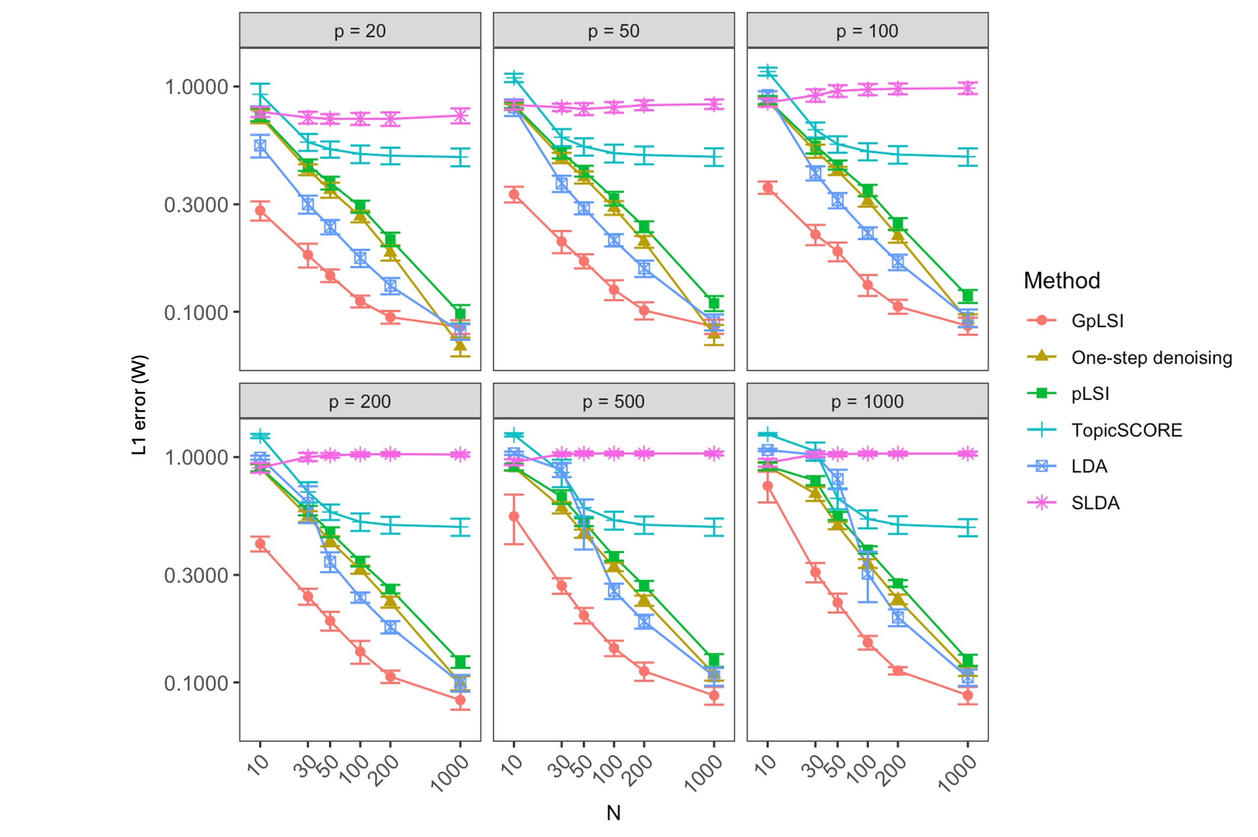
To assess the performance of GpLSI, we compare it against several established methods, including the original pLSI algorithm proposed by Klopp et al. (2021), TopicSCORE (Ke & Wang 2017), LDA (Blei et al. 2001), and the Spatial LDA (SLDA) approach of Chen et al. (2020). In addition, to highlight the efficiency of our iterative algorithm, we present results from a baseline variant that employs only a single denoising step. This one-step method is described in greater detail in Section C of the Appendix. To implement these algorithms, we use the R package TopicScore and the LDA implementation of the Python library sklearn. For SLDA, we use of the Python package spatial-lda with the default settings of the algorithm. We run 50 simulations and record the 1\ell_{1} error, 2\ell_{2} error of WW and AA, and the computation time across various parameter settings (p,N,n,K)(p,N,n,K), reporting medians and interquartile ranges. To evaluate the performance of methods in difficult scenarios where document length NN is small compared to vocabulary size pp, we check the errors for different combinations of N=10,30,50,100,200,1000N=10,30,50,100,200,1000 and p=20,30,50,100,200,500p=20,30,50,100,200,500.

Results

Figure 1 demonstrates that GpLSI achieves the lowest 2\ell_{2} error for WW, even in scenarios with very small NN. This shows that sharing information across similar documents on a graph improves the estimation of topic mixture matrix. Notably, while LDA and pLSI exhibit modest performance, they fail in regimes where N<100N<100 and p200p\geq 200. We also confirm that the one-step denoising variant of our method achieves a lower error estimation error than pLSI and LDA in settings where N<<pN<<p.

Refer to caption
Figure 2: 2\ell_{2} error of WW (left) and AA (middle) and computation time (right) for different corpus size nn and number of topics KK. Here, N=30N=30 and p=30p=30. Errors are normalzied by nn.

We also examine how the estimation errors scale with the corpus size nn and the number of topics KK, as shown in Figure 2. We observe that GpLSI substantially outperforms other methods, particularly for the estimation of WW. GpLSI achieves the lowest error for AA, as we show in Section F of the Appendix. Similar patterns hold for 1\ell_{1} errors of AA and WW also provided in Section F of the Appendix.

4 Real-World Experiments

To highlight the applicability of our method, we deploy it on three real-life examples. All the code for the experiments is openly accessible at https://github.com/yeojin-jung/GpLSI.

4.1 Tumor Microenvironment discovery: the Stanford Colorectal Cancer dataset

We first consider the analysis of CODEX data, which allows the identification of individual cells in tissue samples, holding valuable insights into cell interaction profiles, particularly in cancer, where these interactions are crucial for immune response. Since cellular interactions are hypothesized to be local, these patterns are often referred to as “tumor microenvironments”. In the context of topic modeling, we can regard a tumor microenvironment as a document, immune cell types as words, and latent characteristics of a microenvironment as a topic. However, due to the small number of words per document, the recovery of the topic mixture matrix and the topics themselves can prove challenging. Chen et al. (2020) propose using the adjacency of documents to assign similar topic proportions to neighboring tumor cells. Similarly, we construct a spatial graph based on proximity of tumor microenvironments to uncover novel tumor-immune cell interaction patterns.

The first CODEX dataset is a collection of 292 tissue samples from 161 colorectal cancer patients collected at Stanford University (Wu et al. 2022). The locations of the cells were retrieved using a Voronoi partitioning of the sample, and the corresponding spatial graphs were constructed encoding the distance between microenvironments. More specifically, we define a tumor microenvironment as the 3-hop neighborhood of each cell, following the definition originally used by Wu et al. (2022). Each microenvironment contains 10 to 30 immune cells of 8 possible types. This aligns with the setting where the document length N<30N<30 is small compared to the vocabulary size p=8p=8.

Refer to caption
Figure 3: (A) Estimated tumor-immune topic weights of GpLSI, pLSI, and LDA. Topic weights are aligned across methods using cosine similarity. (B) Topic alignment paths of GpLSI, pLSI, and LDA using R package alto. (C) Pairwise 1\ell_{1} distance and cosine similarity of topic weights from different batches of patients.

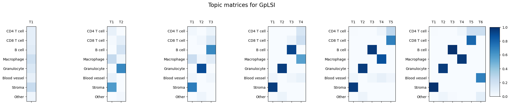
We aggregate frequency matrices and tumor cellular graphs of all samples and fit three methods: our proposed GpLSI, the original pLSI approach of Klopp et al. (2021), and LDA (Blei et al. 2001) to estimate tumor-immune topics. The estimated topic weights of K=6K=6 are illustrated in Figure 3(A). After aligning topic weights across methods, we observe similar immune topics (Topic 1, 2, 3) in GpLSI and LDA which are not found in the estimated topics of pLSI.

To determine the optimal number of topics KK, we use the method proposed by Fukuyama et al. (2023). In this work, the authors construct “topic paths” to track how individual topics evolve, split or merge, as the number of topics KK, increases. We observe in Figure 3(B) that while the GpLSI path has non-overlapping topics up to K=6K=6, other methods fail to provide consistent and well-separated topics.

To evaluate the quality and stability of the recovered topics, we also measure the coherence of the estimated topic weights of batches of samples, as suggested in Tran et al. (2023). We divide 292 samples into five batches and estimate the topic weights AbA^{b} for b[5]b\in[5]. For every pair of batches (b,b)(b,b^{{}^{\prime}}), we align AbA^{b} and AbA^{b^{{}^{\prime}}} (we permute AbA^{b^{{}^{\prime}}} with PP where P=argminP𝒫AbPAbP=\arg\min_{P\in\mathcal{P}}\|A^{b}-PA^{b^{{}^{\prime}}}\|) and measure the entry-wise 1\ell_{1} distance and cosine similarity. We repeat this procedure five times and plot the scores in Figure 3(C). We notice that GpLSI provides the most coherent topics across batches for K=3,4,5K=3,4,5. Combining with the metrics of LDA, we can choose the optimal KK as 5 or 6.

Refer to caption
Figure 4: (A) AUC for predicting cancer recurrence using isometric log-ratio transformed topic proportions (top) and dichotomized topic proportions (bottom) as covariates. (B) Kaplan-Meier curves based on dichotomized topic proportions using GpLSI.

Next, we conduct survival analysis to identify the immune topics associated with higher risk of cancer recurrence. We consider two logistic models with different covariates to predict cancer recurrence and calculate the area under the curve (AUC) of the receiver-operating characteristic (ROC) curves to evaluate model performance.

In the first model, we use the proportion of each microenvironment topic as covariates for each sample. Since the KK covariates sum up to one, we apply isometric log-ratio transformation to represent it with K1K-1 orthonormal basis vectors In the second model, we dichotomize each topic proportion to low and high proportion groups. The cutoffs are determined using the maximally selected rank statistics.

The AUC for each number of topics is shown in Figure 4(A). GpLSI achieves the highest area under the curve (AUC) at K=6K=6 in both models. We also plot Kaplan Meier curves for each topic using the same dichotomized topic proportions. The result for GpLSI is illustrated in Figure 4(B). We observe that Topic 2, which is characterized by a high prevalence of granulocytes, and Topic 6, a mixture of CD4 T cells and blood vessels, are associated with lower cancer recurrence. Positive effect of granulocytes on cancer prognosis was also reported by Wu et al. (2022), who found out that a microenvironment with clustered granulocyte and tumor cells is associated with better patient outcomes. We observe the same association of granulocyte with lower risk in LDA Figure 16 of the Appendix.

4.2 Understanding Structure in Mouse Spleen Samples

Refer to caption
Figure 5: (A) Visualization of estimated B cell microenvironment topics for K=3,5,7,10K=3,5,7,10. (B) Comparison of clustering performance using Moran’s I and PAS score. We plot 1-PAS for better interpretation. (C) Estimated B cell microenvironment topic weights for K=5K=5 using GpLSI.

We also apply our method to identify immune topics in mouse spleen. In this setting, each document is anchored to a B cell (Chen et al. 2020). A previous study has processed the original CODEX images from Goltsev et al. (2018) to obtain the frequencies of non-B cells in the 100 pixel neighborhood of each B cell (Chen et al. 2020). The final input for the topic models consists of a 35,271 B cell microenvironments by 24 cell types frequency matrix, along with the positional data of B cells.

In this example, we evaluate GpLSI by examining whether the introduction of our graph-based regularization term in the estimation of topic mixture matrices enhances document clustering. Figure 5(A) presents the estimated topics for all models at K=3,5,7,10K=3,5,7,10. Notably, the topics derived from GpLSI, pLSI, and LDA more clearly demarcate distinct B cell microenvironment domains compared to those estimated by TopicSCORE and LDA. Among these three methods, GpLSI yields the least noisy cellular clustering, as evidenced by the magnified view of a selected subdomain.

We also evaluate the quality of clusters with two metrics, Moran’s I and the percentage of abnormal spots (PAS) (Shang & Zhou 2022). Moran’s I is a classical measure of spatial autocorrelation that assesses the degree to how values are clustered or dispersed across a spatial domain. PAS score measures the percentage of B cells for which more than 60% of its neighboring B cells have different topics. Higher Moran’s I and lower PAS score indicate more spatial smoothness of the estimated topics. From Figure 5(B), we conclude that GpLSI has the highest Moran I, and the lowest PAS scores, demonstrating improved spatial smoothness of the topics.

We observe that the B cell microenvironment topics identified with GpLSI align well with their biological context (Figure 5(C)). By referencing the manual annotations of B cells from the original study by Goltsev et al. (2018), we infer that Topic 1, Topic 2, Topic 3, and Topic 5 correspond to the red pulp, periarteriolar lymphoid sheath (PALS), B-follicles, and the marginal zone. This interpretation is further supported by high expression of CD4+T cells in Topic 2 (PALS) and high expression of marginal zone macrophages in Topic 5 (marginal zone).

4.3 Analysis of the “What’s Cooking” dataset

This dataset contains recipes from 20 different cuisines across Europe, Asia, and South America. Each recipe is a list of ingredients which allow us to convert to a count matrix with 13,597 recipes (documents) and 1,019 unique ingredients (words). Under the assumption that neighboring countries would have similar cuisine styles, we construct a graph of recipes based on the geographical proximity of the countries. Specifically, for each recipe, we select the five closest recipes from neighboring countries (including its own country) based on the 1\ell_{1} distance of the ingredient count vectors and define them as neighboring nodes on the graph. Through this, we aim to identify general cooking styles that are prevalent across various countries worldwide.

Refer to caption
Figure 6: (A) Estimated anchor ingredients for each topic using GpLSI. (B) Proportion of topics for each cuisine. Each recipe was assigned to a topic with the highest document-topic mixture weight. For each cuisine, we count the number of recipes for each topic and divide by the total number of recipes in the cuisine.

We run GpLSI, pLSI, and LDA with K=5,7,10,15,20K=5,7,10,15,20 topics. We illustrate the estimated topics of GpLSI for K=7K=7 in Figure 6. The results for pLSI and LDA are provided in Section G of the Appendix. With this approach, Topic 1 is clearly a baking topic and Topic 6 is defined by strong spices and sauces common in Mexican or parts of Southeast Asian cuisines. We also observe a general topic for Asian cuisines (Topic 2) and another for Western countries (Topic 7). To evaluate the estimated topics, we compare each topic’s characteristics with the cuisine-by-topic proportion (Figure 6(C)). Indeed, the style of each topic defined by the anchor ingredients aligns with the cuisines that have a high proportion of that topic. For example, the baking topic (Topic 1) is prevalent in British, Irish, French, Russian, and South American cuisines.

In contrast, for pLSI, it is difficult to analyze the characteristics for each topic because Topics 1-4 have one or no identified anchor ingredients. Comparing the cuisine-by-topic proportions of GpLSI and LDA, we observe that GpLSI reveals many cuisines as mixtures of different cooking styles (Figure 6(B)). In contrast, for LDA, many cuisines such as Moroccan, Mexican, Korean, Chinese, Thai have their recipes predominantly classified to a single topic (Figure 18(B) of the Appendix). GpLSI provides estimates of topic mixture and topic weights that are more relevant to our goal of discovering global cooking styles.

5 Conclusion

In this paper, we present Graph-Aligned pLSI (GpLSI), a topic model that leverages document-level metadata to improve estimation of the topic mixture matrix. We incorporate metadata by translating it into document similarity, which is then represented as edges connecting two documents on a graph. GpLSI is a powerful tool that integrates two complementary sources of information: word frequencies that traditional topic models use, and the document graph induced from metadata, which encodes which documents should share similar topic mixture proportions. To the best of our knowledge, this is the first framework to incorporate document-level metadata into topic models with theoretical guarantees.

At the core of GpLSI is an iterative graph-aligned singular value decomposition applied to the observed document-word matrix XX. This procedure projects word frequencies to low-dimensional topic spaces, while ensuring that neighboring documents on the graph share similar topic mixtures. Our SVD approach can also be applied to other works that require dimension reduction with structural constraints on the samples. Additionally, we propose a novel cross validation technique to optimize the level of graph regularization by using the hierarchy of minimum spanning trees to define folds.

Our theoretical analysis and synthetic experiments confirm that GpLSI outperforms existing methods, particularly in “short-document” cases, where the scarcity of words is mitigated by smoothing mixture proportions along neighboring documents. Overall, GpLSI is a fast, highly effective topic model when there is a known structure in the relationship of documents.

We believe that our work offers valuable insights into structural topic models and opens up several avenues for further exploration. A promising direction is to incorporate structure to the topic matrix AA while jointly optimizing structural constraints on WW. While our work focuses on low-pp regime, real world applications, such as genomics data with large pp, could benefit from introducing sparsity to the word composition of each topic.

Appendix for “Graph Topic Modeling for Documents with Spatial or Covariate Dependencies”
Yeo Jin Jung and Claire Donnat

Department of Statistics, The University of Chicago

Appendix A Optimizing graph regularization parameter ρ\rho

In this section, we propose a novel graph cross-validation method which effectively finds the optimal graph regularization parameter by partitioning nodes into folds based on a natural hierarchy derived from a minimum spanning tree. The procedure is summarized in the following algorithm.

Algorithm 2 Cross Validation using Minimum spanning tree at iteration tt
1:Input: Observation XX, incidence matrix Γ\Gamma, minimum spanning tree 𝒯\mathcal{T} of 𝒢\mathcal{G}, previous estimate V^t1\widehat{V}^{t-1}
2:Output: ρ^t\widehat{\rho}^{t}
3:1. Randomly choose the source document dsd_{s}.
4:2. Divide documents into bb folds : dikd_{i}\in\mathcal{I}_{k} if d𝒯(di,ds)modb=k1\emph{d}_{\mathcal{T}}(d_{i},d_{s})\mod b=k-1, for i[n]i\in[n] and k[b]k\in[b].
5:for  each leave-out fold k,k[b]\mathcal{I}_{k},k\in[b] do
6:     Interpolation of XkX^{k} with average of neighbors: Xik=1|𝒩(i)|j𝒩(i)kXjX^{k}_{i\cdot}=\frac{1}{\lvert\mathcal{N}(i)\rvert}\sum_{j\in\mathcal{N}(i)\setminus\mathcal{I}_{k}}X_{j} for iki\in\mathcal{I}_{k}
7:     for ρ{ρ1,ρ2,,ρr}\rho\in\{\rho_{1},\rho_{2},\cdots,\rho_{r}\} do
8:         CVERRk(ρ)=XkU^ρ,k(V^t1)F2\mathrm{CVERR}_{k}(\rho)=\lVert X_{\mathcal{I}_{k}\cdot}-\widehat{U}^{\rho,k}(\widehat{V}^{t-1})^{\top}\rVert_{F}^{2} where
9:         U^ρ,k=argminUUXkV^t1F+ρΓU21\widehat{U}^{\rho,k}=\arg\min_{U}\lVert U-X^{k}\widehat{V}^{t-1}\rVert_{F}+\rho\lVert\Gamma U\rVert_{21}
10:     end for
11:end for
12:4. Choose optimal ρ\rho: ρ^t=argminρkCVERRk(ρ)\hat{\rho}^{t}=\arg\min_{\rho}\sum_{k}\mathrm{CVERR}_{k}(\rho)

Conventional cross validation techniques sample either nodes or edges to divide the dataset into folds. However, these approaches can disrupt the graph structure and underestimate the strength of the connectivity of the graph. We instead devise a new rule for dividing documents into folds using a minimum spanning tree. This technique is an extension of the cross-validation procedure proposed by Tibshirani & Taylor (2012) for the line graph. Given a minimum spanning tree 𝒯\mathcal{T} of 𝒢\mathcal{G}, we randomly choose a source document dsd_{s}. For each document did_{i}, we calculate the shortest path distance d𝒯(di,ds)\mathrm{d}_{\mathcal{T}}(d_{i},d_{s}). Note that this distance is always an integer. We divide the documents into bb folds based on the modulus of their distance from the source node: dT(di,ds)modb\mathrm{d}_{T}(d_{i},d_{s})\mod b. Through this construction of folds, we can ensure that for every document, at least one of its 1-hop neighbors is in a different fold.

Let XiX_{i\cdot} be the ithi^{th} row of XX. For each leave-out fold k\mathcal{I}_{k}, k[b]k\in[b], we interpolate the corresponding documents XiX_{i\cdot}ik\forall i\in\mathcal{I}_{k}, filling the missing document information with the average of corresponding neighbors in kC\mathcal{I}_{k}^{C}. This prevents us from using any information from the leave-out fold in training when calculating the cross-validation error.

Refer to caption
Figure 7: Behavior of ρ^MSTCV\hat{\rho}_{MST-CV} as NN increases (left). Behavior of 2\ell_{2} error over graph heterogeneity (right). Graph heterogeneity is characterized by ngrpn_{grp}, the number of patches of documents across the unit square. Each patch is assigned similar topic mixture weights.

Figure 7 demonstrates how GpLSI leverages the graph information. As NN increases, GpLSI chooses smaller graph regularization parameter ρ^MSTCV\hat{\rho}_{MST-CV}, since the need to share information across neighbors diminishes as documents become longer and more informative. Additionally, when WW is more heterogeneous over the graph—meaning neighboring documents exhibit more heterogeneous topic mixture weights—the 2\ell_{2} error of WW increases. Here, graph heterogeneity is characterized by our simulation parameter ngrpn_{grp} (the number of patches that we create). As ngrpn_{grp} increases, the unit square is divided into finer patches, and the generated documents within the same topic become more dispersed. Our result indicates that GpLSI works well in settings where the mixture weights are smoother over the document graph and the performance of GpLSI and pLSI become similar as neighboring documents become more heterogeneous.

Appendix B Analysis of the initialization step

In this section, we show that the initialization step of GpLSI provides reasonable estimators of UU and VV.

Proof of Theorem 1

Proof.

Let D0D_{0} denote the diagonal matrix where each entry (D0)jj(D_{0})_{jj} is defined as: (D0)jj=1ni=1nMij.(D_{0})_{jj}=\frac{1}{n}\sum_{i=1}^{n}M_{ij}. Let D^0\widehat{D}_{0} denote its empirical counterpart, that is, the diagonal matrix defined as: D^0=diag(1n{i=1nXij}j[p])\widehat{D}_{0}=\text{diag}(\frac{1}{n}\{\sum_{i=1}^{n}X_{ij}\}_{j\in[p]}), so that 𝔼[D^0]=D0\mathbb{E}[\widehat{D}_{0}]=D_{0}. We have, by definition of the initialization procedure:

V^0=UK(XXnND^0),\widehat{V}_{0}=U_{K}(X^{\top}X-\frac{n}{N}\widehat{D}_{0}),

where the notation UK(A)U_{K}(A) denotes the first KK left singular vectors of the matrix AA.

We write X=M+ZX=M+Z, where ZZ denotes some multinomial noise. E We have:

ZZ=i=1nZiZi𝔼[ZZ]=i=1nCov(Zi)=i=1nCov(Xi)\begin{split}{Z^{\top}Z}&=\sum_{i=1}^{n}Z_{i\cdot}^{\top}Z_{i\cdot}\\ \implies\mathbb{E}[{Z^{\top}Z}]&=\sum_{i=1}^{n}\text{Cov}(Z_{i\cdot})=\sum_{i=1}^{n}\text{Cov}(X_{i\cdot})\end{split} (20)

as ZZ is a centered version of XX (Z=XMZ=X-M). Since each row XiX_{i\cdot} is distributed as a Multinomial(1,Mi)(1,M_{i\cdot}):

(Cov(Xi))jj={Mij(1Mij)N if j=jMijMijN if jji=1n(Cov(Xi))jj={iMij(1Mij)N if j=ji=1nMijMijN if jj(\text{Cov}(X_{i\cdot}))_{jj^{\prime}}=\begin{cases}\frac{M_{ij}(1-M_{ij})}{N}\qquad\text{ if }j=j^{\prime}\\ -\frac{M_{ij}M_{ij^{\prime}}}{N}\qquad\text{ if }j\neq j^{\prime}\\ \end{cases}\implies\sum_{i=1}^{n}(\text{Cov}(X_{i\cdot}))_{jj^{\prime}}=\begin{cases}\sum_{i}\frac{M_{ij}(1-M_{ij})}{N}\qquad\text{ if }j=j^{\prime}\\ -\sum_{i=1}^{n}\frac{M_{ij}M_{ij^{\prime}}}{N}\qquad\text{ if }j\neq j^{\prime}\\ \end{cases}

Thus:

𝔼[ZZ]=nND0MMN=nND0VΛ2VN.\begin{split}\mathbb{E}[{Z^{\top}Z}]&=\frac{n}{N}D_{0}-\frac{M^{\top}M}{N}\\ &=\frac{n}{N}D_{0}-\frac{V^{\top}\Lambda^{2}V}{N}.\end{split} (21)

Therefore:

XXnND^0(11N)MM=ZZ+ZM+MZnND^0𝔼[ZZ]+nN𝔼[D^0]\begin{split}{X^{\top}X}-\frac{n}{N}\widehat{D}_{0}-(1-\frac{1}{N}){M^{\top}M}&=Z^{\top}Z+Z^{\top}M+M^{\top}Z-\frac{n}{N}\widehat{D}_{0}-\mathbb{E}[Z^{\top}Z]+\frac{n}{N}\mathbb{E}[\widehat{D}_{0}]\\ \end{split} (22)

Thus 𝔼[XXnND^0]=(11N)MM.\mathbb{E}[{X^{\top}X}-\frac{n}{N}\widehat{D}_{0}]=(1-\frac{1}{N})M^{\top}M. We further note that (11N)MM=VΛ~2V(1-\frac{1}{N})M^{\top}M=V\tilde{\Lambda}^{2}V with Λ~=11NΛ,\tilde{\Lambda}=\sqrt{1-\frac{1}{N}}\Lambda, so the eigenvectors of the matrix XXnND^0{X^{\top}X}-\frac{n}{N}\widehat{D}_{0} can be considered as estimators of those of the matrix MM.M^{\top}M.

By the Davis-Kahan theorem (Giraud 2021):

sinΘ(V,V^0)F2XXnD^0N(11N)MMF(11N)λK(M)22ZZ𝔼[ZZ]F+nND^0𝔼[D^0]F+ZMF+MZF(11N)λK(M)2\begin{split}\|\sin\Theta(V,\widehat{V}^{0})\|_{F}&\leq 2\frac{\|{X^{\top}X}-\frac{n\widehat{D}_{0}}{N}-(1-\frac{1}{N}){M^{\top}M}\|_{F}}{(1-\frac{1}{N})\lambda_{K}(M)^{2}}\\ &\leq 2\frac{\|Z^{\top}Z-\mathbb{E}[Z^{\top}Z]\|_{F}+\frac{n}{N}\|\widehat{D}_{0}-\mathbb{E}[\widehat{D}_{0}]\|_{F}+\|Z^{\top}M\|_{F}+\|M^{\top}Z\|_{F}}{(1-\frac{1}{N})\lambda_{K}(M)^{2}}\\ \end{split} (23)

By Lemma 12, we have with probability at least 1o(n1)1-o(n^{-1}):

ZZ𝔼[ZZ]FC1Knlog(n)N,\|Z^{\top}Z-\mathbb{E}[Z^{\top}Z]\|_{F}\leq C_{1}K\sqrt{\frac{n\log(n)}{N}},
ZMF=MZFC2Knlog(n)N,\|Z^{\top}M\|_{F}=\|M^{\top}Z\|_{F}\leq C_{2}K\sqrt{\frac{n\log(n)}{N}},

and

nND^0𝔼[D^0]FC3NKnlog(n)N.\frac{n}{N}\|\widehat{D}_{0}-\mathbb{E}[\widehat{D}_{0}]\|_{F}\leq\frac{C_{3}}{N}\sqrt{\frac{Kn\log(n)}{N}}.

Thus, assuming N>1N>1, so 111N<2\frac{1}{1-\frac{1}{N}}<2 and 1N12:\frac{1}{N}\leq\frac{1}{2}:

sinΘ(V,V^0)F4CλK(M)2Knlog(n)N\begin{split}\|\sin\Theta(V,\widehat{V}^{0})\|_{F}&\leq\frac{4C}{\lambda_{K}(M)^{2}}K\sqrt{\frac{n\log(n)}{N}}\end{split}

with C=C1C2C3.C=C_{1}\vee C_{2}\vee C_{3}. Under Assumption 4, we have λK(M)cλ1(W)cn/K\lambda_{K}(M)\geq c\lambda_{1}(W)\geq c\sqrt{n/K} (see Lemma 7), therefore:

sinΘ(V,V^0)F4Cc2K2log(n)nN\begin{split}\|\sin\Theta(V,\widehat{V}^{0})\|_{F}&\leq\frac{4C}{c^{2}}K^{2}\sqrt{\frac{\log(n)}{nN}}\\ \end{split}

The condition on NN assumed in Theorem 2 ensures that sinΘ(V,V^0)F<12\|\sin\Theta(V,\widehat{V}^{0})\|_{F}<\frac{1}{2}. ∎

Appendix C Analysis of iterative graph-aligned denoising

Our proof is organized along the following outline:

  1. 1.

    We begin by showing that our graph-total variation penalty yields better estimates of the left and right singular vectors. To this end, we must show that, provided that the initialization is good enough, the estimation error of the singular vectors decreases with the number of iterations.

  2. 2.

    We show that, by a simple readaptation of the proof by Klopp et al. (2021), our estimator—which simply plugs in our singular vector estimates in their procedure —yields a better estimate of the mixture matrix WW.

  3. 3.

    Finally, we show that our estimator of the topic matrix AA yields better error.

C.1 Analysis of the graph-regularized SVD procedure

In this section, we derive high-probability error bounds for the estimates U^\widehat{U} and V^\widehat{V} that we obtain in Algorithm 1. For each t>0t>0, we define the error LtL_{t} at iteration tt as:

Lt=max{sinΘ(V,V^t)F,sinΘ(U,U^t)F}.L_{t}=\max\{\|\sin\Theta(V,\widehat{V}^{t})\|_{F},\|\sin\Theta(U,\widehat{U}^{t})\|_{F}\}. (24)

Our proof operates by recursion. We explicit the dependency of LtL_{t} on the error at the previous iteration Lt1L_{t-1}, and show that {Lt}t=1,,tmax\{L_{t}\}_{t=1,\cdots,t_{\max}} forms a geometric series. To this end, we begin by analyzing the error of the denoised matrix U¯t\bar{U}^{t}, of which we later take an SVD to extract U^t\widehat{U}^{t}.

At each iteration tt, the first step of Algorithm 1 is to consider the following optimization problem:

U¯targminUn×KUXV^t1F2+ρΓU21\bar{U}^{t}\in\arg\min_{U\in\mathbb{R}^{n\times K}}\|{U-X\widehat{V}^{t-1}}\|_{F}^{2}+\rho\|{\Gamma U}\|_{21}\\ (25)

Fix t>0t>0. To simplify notations, we let

Y~=XV^t1,U~=MV^t1,Z~=ZV^t1\tilde{Y}=X\widehat{V}^{t-1},\qquad\tilde{U}=M\widehat{V}^{t-1},\qquad\tilde{Z}=Z\widehat{V}^{t-1} (26)

Note that with these notations, Y~\tilde{Y} can be written as:

Y~=U~+Z~\tilde{Y}=\tilde{U}+\tilde{Z} (27)
Lemma 1 (Error bound of Graph-aligned Denoising).

Let Assumption 1 to 5 hold and let LtL_{t}, U¯t\bar{U}^{t}, Y~\tilde{Y}, U~\tilde{U}, ρ\rho be given as (24)-(27). Assume max(K,p)n\max(K,p)\leq n and Kp\sqrt{K}\leq p. Then, for a choice of ρ=4Cρ(Γ)KpnN(1+Lt1)\rho=4C^{*}\rho(\Gamma)\sqrt{\frac{Kp_{n}}{N}}(1+L_{t-1}) with a constant C>0C^{*}>0, there exists a constant C>0C>0 such that with probability at least 1o(n1)1-o(n^{-1}), for any t>0t>0,

U¯tU~FCKlog(n)N(n𝒞+ρ(Γ)sλmax(L)(1+Lt1))\|\bar{U}^{t}-\tilde{U}\|_{F}\leq C\sqrt{\frac{K\log(n)}{N}}\left(\sqrt{n_{\mathcal{C}}}+\rho(\Gamma)\sqrt{s}\sqrt{\lambda_{\max}(L)}(1+L_{t-1})\right) (28)

where LL denotes the graph Laplacian.

Proof.

By the KKT conditions, the solution U¯t\bar{U}^{t} of (25) verifies :

2(U¯tY~)+ρΓDΓU¯t=0with D=diag({1(ΓUt)e2}e)\begin{split}2(\bar{U}^{t}-\tilde{Y})+\rho\Gamma^{\top}D\Gamma\bar{U}^{t}&=0\qquad\text{with }D=\text{diag}(\{\frac{1}{\|(\Gamma U^{t})_{e\cdot}\|_{2}}\}_{e\in\mathcal{E}})\end{split}

This implies:

Y~U¯t,U¯t=ρ2ΓU¯t,DΓU¯t=ρ2ΓU¯t21andUn×K,Y~U¯t,U=ρ2ΓU,DΓU¯tρ2ΓU21\begin{split}\langle\tilde{Y}-\bar{U}^{t},\bar{U}^{t}\rangle&=\frac{\rho}{2}\langle\Gamma\bar{U}^{t},D\Gamma\bar{U}^{t}\rangle=\frac{\rho}{2}\|\Gamma\bar{U}^{t}\|_{21}\\ \text{and}\quad\forall U\in\mathbb{R}^{n\times K},\qquad\langle\tilde{Y}-\bar{U}^{t},U\rangle&=\frac{\rho}{2}\langle\Gamma U,D\Gamma\bar{U}^{t}\rangle\leq\frac{\rho}{2}\|\Gamma{U}\|_{21}\\ \end{split}

Therefore:

Y~U¯t,UU¯tρ2(ΓU21ΓU¯t21)U~U¯t,UU¯tZ~,U¯tU+ρ2(ΓU21ΓU¯t21)\begin{split}\langle\tilde{Y}-\bar{U}^{t},U-\bar{U}^{t}\rangle&\leq\frac{\rho}{2}(\|\Gamma{U}\|_{21}-\|\Gamma\bar{U}^{t}\|_{21})\\ \langle\tilde{U}-\bar{U}^{t},U-\bar{U}^{t}\rangle&\leq\langle\tilde{Z},\bar{U}^{t}-U\rangle+\frac{\rho}{2}(\|\Gamma{U}\|_{21}-\|\Gamma\bar{U}^{t}\|_{21})\\ \end{split}

Using the polarization inequality:

UU¯tF2+U~U¯tF2U~UF2+2Z~,U¯tU+ρ(ΓU21ΓU¯t21)\begin{split}\|U-\bar{U}^{t}\|_{F}^{2}+\|\tilde{U}-\bar{U}^{t}\|_{F}^{2}&\leq\|\tilde{U}-{U}\|_{F}^{2}+2\langle\tilde{Z},\bar{U}^{t}-U\rangle+\rho(\|\Gamma{U}\|_{21}-\|\Gamma\bar{U}^{t}\|_{21})\\ \end{split}

and, choosing U=U~:U=\tilde{U}:

U~U¯tF2Z~,U¯tU~+ρ2(ΓU~21ΓU¯t21)\|\tilde{U}-\bar{U}^{t}\|_{F}^{2}\leq\langle\tilde{Z},\bar{U}^{t}-\tilde{U}\rangle+\frac{\rho}{2}(\|\Gamma\tilde{U}\|_{21}-\|\Gamma\bar{U}^{t}\|_{21})

Let Δ=U~U¯t\Delta=\tilde{U}-\bar{U}^{t}. By the triangle inequality, the right-most term in the above inequality can be rewritten as:

ΓU~21ΓU¯t21=(ΓU~)𝒮21+(ΓU~)𝒮C21(ΓU~+ΓΔ)𝒮21(ΓU~+ΓΔ)𝒮C21(ΓΔ)𝒮21(ΓΔ)𝒮C21,\begin{split}\|\Gamma\tilde{U}\|_{21}-\|\Gamma\bar{U}^{t}\|_{21}&=\|(\Gamma\tilde{U})_{\mathcal{S}\cdot}\|_{21}+\|(\Gamma\tilde{U})_{\mathcal{S}^{C}\cdot}\|_{21}-\|(\Gamma\tilde{U}+\Gamma\Delta)_{\mathcal{S}\cdot}\|_{21}-\|(\Gamma\tilde{U}+\Gamma\Delta)_{\mathcal{S}^{C}\cdot}\|_{21}\\ &\leq\|(\Gamma\Delta)_{\mathcal{S}\cdot}\|_{21}-\|(\Gamma\Delta)_{\mathcal{S}^{C}\cdot}\|_{21},\\ \end{split}

since by assumption, (ΓU~)𝒮C21=0.\|(\Gamma\tilde{U})_{\mathcal{S}^{C}\cdot}\|_{21}=0.

We turn to the control of the error term Z~,U¯tU~\langle\tilde{Z},\bar{U}^{t}-\tilde{U}\rangle. Using the decomposition of n\mathbb{R}^{n} induced by the projection ΓΓ\Gamma^{\dagger}\Gamma as In=ΠΓΓI_{n}=\Pi\oplus^{\perp}\Gamma^{\dagger}\Gamma, we have:

Z~,U¯tU~=Z~,Π(U¯tU~)+Z~,ΓΓ(U¯tU~)=ΠZ~,ΠΔ(A)+(Γ)Z~,ΓΔ(B).\begin{split}\langle\tilde{Z},\bar{U}^{t}-\tilde{U}\rangle&=\langle\tilde{Z},\Pi(\bar{U}^{t}-\tilde{U})\rangle+\langle\tilde{Z},\Gamma^{\dagger}\Gamma(\bar{U}^{t}-\tilde{U})\rangle\\ &=\underbrace{\langle\Pi\tilde{Z},\Pi\Delta\rangle}_{(A)}+\underbrace{\langle(\Gamma^{\dagger})^{\top}\tilde{Z},\Gamma\Delta\rangle}_{(B)}.\end{split} (29)
Bound on (A) in Equation (29)

By Cauchy-Schwarz:

ΠZ~,ΠΔΠZ~FΠΔF\begin{split}\langle\Pi\tilde{Z},\Pi\Delta\rangle&\leq\|\Pi\tilde{Z}\|_{F}\|\Pi\Delta\|_{F}\end{split}

By Lemma 16, with probability at least 1o(n1)1-o(n^{-1}):

ΠZ~F2C1n𝒞Klog(n)N\|\Pi\tilde{Z}\|_{F}^{2}\leq C_{1}n_{\mathcal{C}}K\frac{\log(n)}{N}
Bound on (B) in Equation (29).
(Γ)Z~,ΓΔ=e[m]((Γ)Z~)e,(ΓΔ)ee[m]((Γ)Z~)e2(ΓΔ)e2by Cauchy-Schwarzmaxe[m](Γ)Z~)e2e[m](ΓΔ)e2=maxe[m]((Γ)Z~)e2ΓΔ21\begin{split}\langle(\Gamma^{\dagger})^{\top}\tilde{Z},\Gamma\Delta\rangle&=\sum_{e\in[m]}\langle((\Gamma^{\dagger})^{\top}\tilde{Z})_{e\cdot},(\Gamma\Delta)_{e\cdot}\rangle\\ &\leq\sum_{e\in[m]}\|((\Gamma^{\dagger})^{\top}\tilde{Z})_{e\cdot}\|_{2}\|(\Gamma\Delta)_{e\cdot}\|_{2}\qquad\text{by Cauchy-Schwarz}\\ &\leq\max_{e\in[m]}\|(\Gamma^{\dagger})^{\top}\tilde{Z})_{e\cdot}\|_{2}\sum_{e\in[m]}\|(\Gamma\Delta)_{e\cdot}\|_{2}\\ &=\max_{e\in[m]}\|((\Gamma^{\dagger})^{\top}\tilde{Z})_{e\cdot}\|_{2}\|\Gamma\Delta\|_{21}\\ \end{split}

Thus, on the event 𝒜={ρ4maxe[m](Γ)Z~)e2}\mathcal{A}=\{\rho\geq 4\max_{e\in[m]}\|(\Gamma^{\dagger})^{\top}\tilde{Z})_{e\cdot}\|_{2}\}, we have:

(Γ)Z~,ΓΔρ4ΓΔ21.\begin{split}\langle(\Gamma^{\dagger})^{\top}\tilde{Z},\Gamma\Delta\rangle&\leq\frac{\rho}{4}\|\Gamma\Delta\|_{21}.\\ \end{split}

To derive (𝒜)\mathbb{P}(\mathcal{A}), we first establish the relationship between Z~\tilde{Z} and Lt1L_{t-1},

Z~=Z(PV+PV)V^t1=ZVVV^t1+ZVVV^t1\tilde{Z}=Z(P_{V}+P_{V_{\perp}})\widehat{V}^{t-1}=ZVV^{\top}\widehat{V}^{t-1}+ZV_{\perp}V_{\perp}^{\top}\widehat{V}^{t-1}

Then,

maxe[m](Γ)Z~)e2=maxe[m](Γ)(ZVVV^t1+ZVVV^t1))e2maxe[m]((Γ)Z)e2VV^t1op+maxe[m]((Γ)Z)e2VV^t1opmaxe[m]((Γ)Z)e2(1+Lt1)\begin{split}\max_{e\in[m]}\|(\Gamma^{\dagger})^{\top}\tilde{Z})_{e\cdot}\|_{2}&=\max_{e\in[m]}\|(\Gamma^{\dagger})^{\top}(ZVV^{\top}\widehat{V}^{t-1}+ZV_{\perp}V_{\perp}^{\top}\widehat{V}^{t-1}))_{e\cdot}\|_{2}\\ &\leq\max_{e\in[m]}\|((\Gamma^{\dagger})^{\top}Z)_{e\cdot}\|_{2}\|V^{\top}\widehat{V}^{t-1}\|_{op}+\max_{e\in[m]}\|((\Gamma^{\dagger})^{\top}Z)_{e\cdot}\|_{2}\|V_{\perp}^{\top}\widehat{V}^{t-1}\|_{op}\\ &\leq\max_{e\in[m]}\|((\Gamma^{\dagger})^{\top}Z)_{e\cdot}\|_{2}(1+L_{t-1})\end{split}

where we used the fact sinΘ(V,V^t1)F=VV^t1FVV^t1op\|\sin\Theta(V,\widehat{V}^{t-1})\|_{F}=\|V_{\perp}^{\top}\widehat{V}^{t-1}\|_{F}\geq\|V_{\perp}^{\top}\widehat{V}^{t-1}\|_{op}. From Lemma 13, for a choice of ρ=4Cρ(Γ)Klog(n)N(1+Lt1)\rho=4C^{*}\rho(\Gamma)\sqrt{\frac{K\log(n)}{N}}(1+L_{t-1}), then [𝒜]1o(n1)\mathbb{P}\left[\mathcal{A}\right]\geq 1-o(n^{-1}).

Therefore:

ΔF2ΠZ~FΔF+3ρ4ΓΔ21ΠZ~FΔF+3ρ4sΓΔFΠZ~FΔF+3ρ4sλmax(Γ)ΔF\begin{split}\|\Delta\|_{F}^{2}&\leq\|\Pi\tilde{Z}\|_{F}\|\Delta\|_{F}+\frac{3\rho}{4}\|\Gamma\Delta\|_{21}\\ &\leq\|\Pi\tilde{Z}\|_{F}\|\Delta\|_{F}+\frac{3\rho}{4}\sqrt{s}\|\Gamma\Delta\|_{F}\\ &\leq\|\Pi\tilde{Z}\|_{F}\|\Delta\|_{F}+\frac{3\rho}{4}\sqrt{s}{\lambda_{\max}(\Gamma)}\|\Delta\|_{F}\\ \end{split} (30)

and thus:

U~U¯tFC1n𝒞Klog(n)N+3C2ρ(Γ)sλmax(Γ)Klog(n)N(1+Lt1)CKlog(n)N(n𝒞+ρ(Γ)sλmax(Γ)(1+Lt1))\begin{split}\|\tilde{U}-\bar{U}^{t}\|_{F}&\leq C_{1}\sqrt{\frac{n_{\mathcal{C}}K\log(n)}{N}}+3C_{2}\rho(\Gamma)\sqrt{s}{\lambda_{\max}(\Gamma)}\sqrt{\frac{K\log(n)}{N}}(1+L_{t-1})\\ &\leq C\sqrt{\frac{K\log(n)}{N}}(\sqrt{n_{\mathcal{C}}}+\rho(\Gamma)\sqrt{s}{\lambda_{\max}(\Gamma)}(1+L_{t-1}))\\ \end{split}

The result follows by noting that the Laplacian of the graph LL is linked to Γ\Gamma by L=ΓΓL=\Gamma^{\top}\Gamma. ∎

Proof of Theorem 2

Proof.

Recall LtL_{t}, the error at each iteration tt:

Lt=max{sinΘ(V,V^t)F,sinΘ(U,U^t)F}.L_{t}=\max\{\|\sin\Theta(V,\widehat{V}^{t})\|_{F},\|\sin\Theta(U,\widehat{U}^{t})\|_{F}\}. (31)
Bound on sin(Θ(U,U^t)F\|\sin(\Theta(U,\widehat{U}^{t})\|_{F}.

We start by deriving a bound for sinΘ(U,U^t)F\|\sin\Theta(U,\widehat{U}^{t})\|_{F}. Let UU_{\perp} denote the orthogonal complement of U,U, so that:

In=UU+UU.I_{n}=UU^{\top}+U_{\perp}U_{\perp}^{\top}.

Noting that U^t\widehat{U}^{t} is the matrix corresponding to the top KK left singular vectors of the matrix U~t=(U~tMV)+MV=(U~tMV^t+MV^tMV)+MV,\tilde{U}^{t}=(\tilde{U}^{t}-MV)+MV=(\tilde{U}^{t}-M\widehat{V}^{t}+M\widehat{V}^{t}-MV)+MV, by Theorem 1 of Cai & Zhang (2018) (which we rewrote in Lemma  8 of this manuscript to make it self-contained):

sinΘ(U,U^t)FPU(U~tMV^t+MV^tMV)Fλmin(UU~t)=PU(U~tMV^t)Fλmin(UU~t)\begin{split}\|\sin\Theta(U,\widehat{U}^{t})\|_{F}&\leq\frac{\|P_{U_{\perp}}(\tilde{U}^{t}-M\widehat{V}^{t}+M\widehat{V}^{t}-MV)\|_{F}}{\lambda_{\min}(U^{\top}\tilde{U}^{t})}\\ &=\frac{\|P_{U_{\perp}}(\tilde{U}^{t}-M\widehat{V}^{t})\|_{F}}{\lambda_{\min}(U^{\top}\tilde{U}^{t})}\end{split}

where the second line follows from noting that PU(MV^tMV)=0.P_{U_{\perp}}(M\widehat{V}^{t}-MV)=0.

Since Λ\Lambda is a diagonal matrix, we have:

λmin(UMV^t1)=λmin(ΛVV^t1)=minuK,vp:u=v=1uΛVV^t1v=λK(M)minuK,vp:u=v=1uVV^t1v=λK(M)λmin(VV^t1)\begin{split}\lambda_{\min}(U^{\top}M\widehat{V}^{t-1})=\lambda_{\min}(\Lambda V^{\top}\widehat{V}^{t-1})&=\min_{u\in\mathbb{R}^{K},v\in\mathbb{R}^{p}:\|u\|=\|v\|=1}u^{\top}\Lambda V^{\top}\widehat{V}^{t-1}v\\ &=\lambda_{K}(M)\min_{u\in\mathbb{R}^{K},v\in\mathbb{R}^{p}:\|u\|=\|v\|=1}u^{\top}V^{\top}\widehat{V}^{t-1}v\\ &=\lambda_{K}(M)\lambda_{\min}(V^{\top}\widehat{V}^{t-1})\end{split}

Thus, by Weyl’s inequality:

λmin(UU~t)=λmin(U(U~tMV^t1+MV^t1))λmax(U(U~tMV^t1))+λmin(UMV^t1)λmin(ΛVV^t1)U~tMV^t1F=λK(M)1Lt12ΔF\begin{split}\lambda_{\min}(U^{\top}\tilde{U}^{t})&=\lambda_{\min}(U^{\top}(\tilde{U}^{t}-M\widehat{V}^{t-1}+M\widehat{V}^{t-1}))\\ &\geq-\lambda_{\max}(U^{\top}(\tilde{U}^{t}-M\widehat{V}^{t-1}))+\lambda_{\min}(U^{\top}M\widehat{V}^{t-1})\\ &\geq\lambda_{\min}(\Lambda V^{\top}\widehat{V}^{t-1})-\|\tilde{U}^{t}-M\widehat{V}^{t-1}\|_{F}=\lambda_{K}(M)\sqrt{1-L_{t-1}^{2}}-\|\Delta\|_{F}\\ \end{split}

where Δ=U~tMV^t1.\Delta=\tilde{U}^{t}-M\widehat{V}^{t-1}. By Lemma 1, we know that:

ΔFCKlog(n)N(n𝒞+ρ(Γ)sλmax(1+Lt1))=ηn+δnLt1\|\Delta\|_{F}\leq C\sqrt{\frac{K\log(n)}{N}}\left(\sqrt{n_{\mathcal{C}}}+\rho(\Gamma)\sqrt{s}\sqrt{\lambda_{\max}}(1+L_{t-1})\right)=\eta_{n}+\delta_{n}L_{t-1}

with ηn=CKlog(n)N(n𝒞+ρ(Γ)sλmax(Γ))\eta_{n}=C\sqrt{\frac{K\log(n)}{N}}\left(\sqrt{n_{\mathcal{C}}}+\rho(\Gamma)\sqrt{s}\sqrt{\lambda_{\max}(\Gamma)}\right) and δn=Cρ(Γ)sλmax(Γ)Klog(n)N.\delta_{n}=C\rho(\Gamma)\sqrt{s\lambda_{\max}(\Gamma)\frac{K\log(n)}{N}}. Thus:

sinΘ(U,U^t)FΔFλK(M)1Lt12ΔFηn+δnLt1λK(M)1Lt12(ηn+δnLt1)ηn+δnLt1λK(M)/2(ηn+δnLt1)\begin{split}\|\sin\Theta(U,\widehat{U}^{t})\|_{F}&\leq\frac{\|\Delta\|_{F}}{\lambda_{K}(M)\sqrt{1-L_{t-1}^{2}}-\|\Delta\|_{F}}\\ &\leq\frac{\eta_{n}+\delta_{n}L_{t-1}}{\lambda_{K}(M)\sqrt{1-L_{t-1}^{2}}-(\eta_{n}+\delta_{n}L_{t-1})}\\ &\leq\frac{\eta_{n}+\delta_{n}L_{t-1}}{\lambda_{K}(M)/2-(\eta_{n}+\delta_{n}L_{t-1})}\\ \end{split}

where the last line follows by assuming that Lt112t0L_{t-1}\leq\frac{1}{2}\quad\forall t\geq 0 (we will show that this indeed holds). By using a first-order Taylor expansion around 0 for the function f(x)=a+bxcabxf(x)=\frac{a+bx}{c-a-bx} for x(0,1/2)x\in(0,1/2), we obtain:

f(x)<aca+bc(cab/2)2x,for x(0,1/2).f(x)<\frac{a}{c-a}+\frac{bc}{(c-a-b/2)^{2}}x,\quad\text{for }x\in(0,1/2).

Therefore, seeing that we have ηnδn\eta_{n}\geq\delta_{n} and letting u=ηnλK(M)/2ηn=2ηnλK(M)2ηnu=\frac{\eta_{n}}{\lambda_{K}(M)/2-\eta_{n}}=\frac{2\eta_{n}}{\lambda_{K}(M)-2\eta_{n}} and r=λK(M)/2δn(λK(M)/2ηnδn/2)2=2λK(M)δn(λK(M)2ηnδn)22λK(M)ηn(λK(M)3ηn)2r=\frac{\lambda_{K}(M)/2\delta_{n}}{(\lambda_{K}(M)/2-\eta_{n}-\delta_{n}/2)^{2}}=\frac{2\lambda_{K}(M)\delta_{n}}{(\lambda_{K}(M)-2\eta_{n}-\delta_{n})^{2}}\leq\frac{2\lambda_{K}(M)\eta_{n}}{(\lambda_{K}(M)-3\eta_{n})^{2}}, we have:

sinΘ(U,U^t)Fu+rLt1\begin{split}\|\sin\Theta(U,\widehat{U}^{t})\|_{F}&\leq u+rL_{t-1}\\ \end{split}

By Assumption 4, we have λK(M)cnK\lambda_{K}(M)\geq c\sqrt{\frac{n}{K}}. Therefore, λK(M)10ηn\lambda_{K}(M)\geq 10\eta_{n} as soon as:

n100C2c2K2log(n)N(n𝒞+ρ2(Γ)sλmax(Γ))N100C2c2K2log(n)n(n𝒞+ρ2(Γ)sλmax(Γ))\begin{split}n&\geq\frac{100C^{2}}{c^{2}}{\frac{K^{2}\log(n)}{N}}\left({n_{\mathcal{C}}}+\rho^{2}(\Gamma)s\lambda_{\max}(\Gamma)\right)\\ \implies N&\geq\frac{100C^{2}}{c^{2}}\frac{K^{2}\log(n)}{n}\left({n_{\mathcal{C}}}+\rho^{2}(\Gamma)s\lambda_{\max}(\Gamma)\right)\end{split} (32)

which is satisfied under the condition (12) of NN in Theorem 2. Thus, in this setting:

r2λK(M)ηn(λK(M)3ηn)22λK(M)ηn(710λK(M))2200/49ηnλK(M)204912.r\leq\frac{2\lambda_{K}(M)\eta_{n}}{(\lambda_{K}(M)-3\eta_{n})^{2}}\leq\frac{2\lambda_{K}(M)\eta_{n}}{(\frac{7}{10}\lambda_{K}(M))^{2}}\leq\frac{200/49\eta_{n}}{\lambda_{K}(M)}\leq\frac{20}{49}\leq\frac{1}{2}. (33)

and

u2ηnλK(M)2ηn5/2ηnλK(M)520=14u\leq\frac{2\eta_{n}}{\lambda_{K}(M)-2\eta_{n}}\leq\frac{5/2\eta_{n}}{\lambda_{K}(M)}\leq\frac{5}{20}=\frac{1}{4}

Also given that Lt112L_{t-1}\leq\frac{1}{2},

sinΘ(U,U^t)Fu+rLt15/2ηn+100/49ηnλK(M)12.\|\sin\Theta(U,\widehat{U}^{t})\|_{F}\leq u+rL_{t-1}\leq\frac{5/2\eta_{n}+100/49\eta_{n}}{\lambda_{K}(M)}\leq\frac{1}{2}.
Bound on sinΘ(V,V^t)F\|\sin\Theta(V,\widehat{V}^{t})\|_{F}

By definition of the second step:

V^t=UK(XU^t).\widehat{V}^{t}=U_{K}(X^{\top}\widehat{U}^{t}).

By Theorem 1 of Cai & Zhang (2018) (summarized for our use case in Lemma 8):

sinΘ(V,V^t)FPV(M(U^tU)+ZU^t)Fλmin(VXU^t)=PV(ZU^t)Fλmin(VXU^t) since PVM(U^tU)=0\begin{split}\|\sin\Theta(V,\widehat{V}^{t})\|_{F}&\leq\frac{\|P_{V_{\perp}}(M^{\top}(\widehat{U}^{t}-U)+Z^{\top}\widehat{U}^{t})\|_{F}}{\lambda_{\min}(V^{\top}X^{\top}\widehat{U}^{t})}\\ &=\frac{\|P_{V_{\perp}}(Z^{\top}\widehat{U}^{t})\|_{F}}{\lambda_{\min}(V^{\top}X^{\top}\widehat{U}^{t})}\qquad\text{ since }P_{V_{\perp}}M^{\top}(\widehat{U}^{t}-U)=0\end{split}

We have:

λmin(VXU^t)=λmin(VMU^t+VZU^t)λmin(ΛUU^t)λmax(VZU^t) (Weyl’s inequality)=λK(M)λmin(UU^t)=1Lt2VZU^tFλK(M)1Lt2VZU^tF\begin{split}\lambda_{\min}(V^{\top}X^{\top}\widehat{U}^{t})&=\lambda_{\min}(V^{\top}M^{\top}\widehat{U}^{t}+V^{\top}Z^{\top}\widehat{U}^{t})\\ &\geq\lambda_{\min}(\Lambda U^{\top}\widehat{U}^{t})-\lambda_{\max}(V^{\top}Z^{\top}\widehat{U}^{t})\qquad\text{ (Weyl's inequality)}\\ &=\lambda_{K}(M)\underbrace{\lambda_{\min}(U^{\top}\widehat{U}^{t})}_{=\sqrt{1-L_{t}^{2}}}-\|V^{\top}Z^{\top}\widehat{U}^{t}\|_{F}\\ &\geq\lambda_{K}(M)\sqrt{1-L_{t}^{2}}-\|V^{\top}Z^{\top}\widehat{U}^{t}\|_{F}\end{split}

Thus, assuming that Lt12,tL_{t}\leq\frac{1}{2},\forall t:

sinΘ(V,V^t)FVZU^tF12λK(M)VZU^tF.\begin{split}\|\sin\Theta(V,\widehat{V}^{t})\|_{F}&\leq\frac{\|V_{\perp}^{\top}Z^{\top}\widehat{U}^{t}\|_{F}}{\frac{1}{2}\lambda_{K}(M)-\|V^{\top}Z^{\top}\widehat{U}^{t}\|_{F}}.\end{split}

Furthermore:

VZU^tFVZUUU^tF+VZUUU^tFVZUFUU^top+VZUopUU^tFCKlog(n)N+CKnlog(n)NsinΘ(U,U^t)F\begin{split}\|V^{\top}Z^{\top}\widehat{U}^{t}\|_{F}&\leq\|V^{\top}Z^{\top}UU^{\top}\widehat{U}^{t}\|_{F}+\|V^{\top}Z^{\top}U_{\perp}U_{\perp}^{\top}\widehat{U}^{t}\|_{F}\\ &\leq\|V^{\top}Z^{\top}U\|_{F}\|U^{\top}\widehat{U}^{t}\|_{op}+\|V^{\top}Z^{\top}U_{\perp}\|_{op}\|U_{\perp}^{\top}\widehat{U}^{t}\|_{F}\\ &\leq CK\sqrt{\frac{\log(n)}{N}}+C\sqrt{\frac{Kn\log(n)}{N}}\|\sin\Theta(U,\widehat{U}^{t})\|_{F}\end{split}

where the last inequality follows by noting that UU^tF1\|U^{\top}\widehat{U}^{t}\|_{F}\leq 1 and from Lemma 15, which show that with probability at least 1o(1n)1-o(\frac{1}{n}):

ZUFCKlog(n)N\|Z^{\top}{U}\|_{F}\leq CK\sqrt{\frac{\log(n)}{N}}

and since Un×(nK)U_{\perp}\in\mathbb{R}^{n\times(n-K)}:

ZUopCKnlog(n)N.\ \|Z^{\top}{U}_{\perp}\|_{op}\leq C\sqrt{Kn\frac{\log(n)}{N}}.

Therefore, using the same arguments as in the previous paragraph, using η~n=CKlog(n)N\tilde{\eta}_{n}=CK\sqrt{\frac{\log(n)}{N}} and δ~n=CKnlog(n)N\tilde{\delta}_{n}=C\sqrt{\frac{Kn\log(n)}{N}}, we have:

f(x)<aca+bc(cab/2)2x,for x(0,1/2).f(x)<\frac{a}{c-a}+\frac{bc}{(c-a-b/2)^{2}}x,\quad\text{for }x\in(0,1/2).

Therefore, we have η~nδ~n\tilde{\eta}_{n}\leq\tilde{\delta}_{n}, and letting u~=η~nλK(M)/2η~n\tilde{u}=\frac{\tilde{\eta}_{n}}{\lambda_{K}(M)/2-\tilde{\eta}_{n}} and r~=λK(M)/2δ~n(λK(M)/2η~nδ~n/2)2=2λK(M)δ~n(λK(M)2η~nδ~n)22λK(M)δ~n(λK(M)3δ~n)2\tilde{r}=\frac{\lambda_{K}(M)/2\tilde{\delta}_{n}}{(\lambda_{K}(M)/2-\tilde{\eta}_{n}-\tilde{\delta}_{n}/2)^{2}}=\frac{2\lambda_{K}(M)\tilde{\delta}_{n}}{(\lambda_{K}(M)-2\tilde{\eta}_{n}-\tilde{\delta}_{n})^{2}}\leq\frac{2\lambda_{K}(M)\tilde{\delta}_{n}}{(\lambda_{K}(M)-3\tilde{\delta}_{n})^{2}},

sinΘ(V,V^t)Fu~+r~sinΘ(U,U^t)Fu~+r~Lt1\begin{split}\|\sin\Theta(V,\widehat{V}^{t})\|_{F}&\leq\tilde{u}+\tilde{r}\|\sin\Theta(U,\widehat{U}^{t})\|_{F}\leq\tilde{u}+\tilde{r}L_{t-1}\\ \end{split}

when LtL_{t} decreases with each iteration. Again, we note that λK(M)10δ~n\lambda_{K}(M)\geq 10\tilde{\delta}_{n} as soon as:

n100C2c2K2nlog(n)NN100C2c2K2log(n)\begin{split}n&\geq\frac{100C^{2}}{c^{2}}{\frac{K^{2}n\log(n)}{N}}\\ \implies N&\geq\frac{100C^{2}}{c^{2}}{{K^{2}\log(n)}}\end{split} (34)

which is satisfied under the condition (12) of NN in Theorem 2. Then we can show that,

r~2λK(M)δ~n(λK(M)3δ~n)22λK(M)δ~n(710λK(M))2200/49δ~nλK(M)12\tilde{r}\leq\frac{2\lambda_{K}(M)\tilde{\delta}_{n}}{(\lambda_{K}(M)-3\tilde{\delta}_{n})^{2}}\leq\frac{2\lambda_{K}(M)\tilde{\delta}_{n}}{(\frac{7}{10}\lambda_{K}(M))^{2}}\leq\frac{200/49\tilde{\delta}_{n}}{\lambda_{K}(M)}\leq\frac{1}{2} (35)

and

u~2δ~nλK(M)2δ~n5/2δ~nλK(M)520=14\tilde{u}\leq\frac{2\tilde{\delta}_{n}}{\lambda_{K}(M)-2\tilde{\delta}_{n}}\leq\frac{5/2\tilde{\delta}_{n}}{\lambda_{K}(M)}\leq\frac{5}{20}=\frac{1}{4}

Also given that Lt112L_{t-1}\leq\frac{1}{2},

sinΘ(V,V^t)Fu~+r~Lt15/2δ~n+100/49δ~nλK(M)12\|\sin\Theta(V,\widehat{V}^{t})\|_{F}\leq\tilde{u}+\tilde{r}L_{t-1}\leq\frac{5/2\tilde{\delta}_{n}+100/49\tilde{\delta}_{n}}{\lambda_{K}(M)}\leq\frac{1}{2}

and

u~1r~3δ~nλK(M)×λK(M)λK(M)4δ~n12.\frac{\tilde{u}}{1-\tilde{r}}\leq\frac{3\tilde{\delta}_{n}}{\lambda_{K}(M)}\times\frac{\lambda_{K}(M)}{\lambda_{K}(M)-4\tilde{\delta}_{n}}\leq\frac{1}{2}.

Therefore, for all tt,

Lt12.L_{t}\leq\frac{1}{2}.
Behavior of LtL_{t}

LtL_{t} is a decreasing function of tt for t1t\geq 1, and by Theorem 1, L012L_{0}\leq\frac{1}{2} (We later show in (49)). From the previous sections,

sinΘ(U,U^t)F5/2ηnλK(M)+200/49δnλK(M)Lt15/2CλK(M)Klog(n)N(n𝒞+ρ(Γ)sλmax(Γ))+200/49CλK(M)Klog(n)Nρ(Γ)sλmax(Γ)Lt1sinΘ(V,V^t)F5/2η~nλK(M)+200/49δ~nλK(M)Lt15/2CλK(M)Klog(n)N+200/49CλK(M)Knlog(n)NLt1\begin{split}\|\sin\Theta(U,\widehat{U}^{t})\|_{F}&\leq\frac{5/2\eta_{n}}{\lambda_{K}(M)}+\frac{200/49\delta_{n}}{\lambda_{K}(M)}L_{t-1}\\ &\leq\frac{5/2C}{\lambda_{K}(M)}\sqrt{\frac{K\log(n)}{N}}\left(\sqrt{n_{\mathcal{C}}}+\rho(\Gamma)\sqrt{s\lambda_{\max}(\Gamma)}\right)\\ &\qquad+\frac{200/49C}{\lambda_{K}(M)}\sqrt{\frac{K\log(n)}{N}}\rho(\Gamma)\sqrt{s\lambda_{\max}(\Gamma)}L_{t-1}\\ \|\sin\Theta(V,\widehat{V}^{t})\|_{F}&\leq\frac{5/2\tilde{\eta}_{n}}{\lambda_{K}(M)}+\frac{200/49\tilde{\delta}_{n}}{\lambda_{K}(M)}L_{t-1}\\ &\leq\frac{5/2C}{\lambda_{K}(M)}K\sqrt{\frac{\log(n)}{N}}+\frac{200/49C}{\lambda_{K}(M)}\sqrt{\frac{Kn\log(n)}{N}}L_{t-1}\end{split}

Thus,

Ltu+rLt1u+r(u+rLt2)rtL0+u(1+r+r2+rt1)rtL0+u1rt1r\begin{split}L_{t}&\leq u+rL_{t-1}\\ &\leq u+r(u+rL_{t-2})\\ &\leq r^{t}L_{0}+u(1+r+r^{2}+\cdots r^{t-1})\\ &\leq r^{t}L_{0}+u\frac{1-r^{t}}{1-r}\end{split} (36)

where

u=5/2CλK(M)Klog(n)N(n𝒞+ρ(Γ)sλmax(Γ))r=200/49CλK(M)Klog(n)N(ρ(Γ)sλmax(Γ)n)\begin{split}u&=\frac{5/2C}{\lambda_{K}(M)}\sqrt{\frac{K\log(n)}{N}}\left(\sqrt{n_{\mathcal{C}}}+\rho(\Gamma)\sqrt{s\lambda_{\max}(\Gamma)}\right)\\ r&=\frac{200/49C}{\lambda_{K}(M)}\sqrt{\frac{K\log(n)}{N}}\left(\rho(\Gamma)\sqrt{s\lambda_{\max}(\Gamma)}\vee\sqrt{n}\right)\end{split}

where r12,r\leq\frac{1}{2}, In particular, we want to find tmaxt_{\max} such that rtmaxL0r^{t_{\max}}L_{0} becomes small enough to satisfy rtmaxL0u1rr^{t_{\max}}L_{0}\leq\frac{u}{1-r}. Using r12r\leq\frac{1}{2} (as previously shown) and that L012L_{0}\leq\frac{1}{2},

rtmax2u1rtmaxlog(2u)+log(1r)|log(r)|2log(2)log(u)log(2)\begin{split}\frac{r^{t_{\max}}}{2}&\leq\frac{u}{1-r}\\ \implies t_{\max}&\geq\frac{-\log(2u)+\log(1-r)}{|\log(r)|}\geq\frac{-2\log(2)-\log(u)}{\log(2)}\end{split}

Combining with the previous inequality (and since log(2)14\log(2)\leq\frac{1}{4}) and the fact that under Assumption 4, we have λK(M)cn/K\lambda_{K}(M)\geq c\sqrt{n/K}, we can choose tmaxt_{\max} as,

tmax=(2log(nN)4log(5/2Cc)4log(K)2log(logn)4log(n𝒞+ρ(Γ)sλmax(Γ))2)1t_{\max}=\left(2\log(nN)-4\log(\frac{5/2C}{c})-4\log(K)-2\log(\log n)-4\log(\sqrt{n_{\mathcal{C}}}+\rho(\Gamma)\sqrt{s\lambda_{\max}(\Gamma)})-2\right)\vee 1

Thus, it is sufficient to choose tmaxt_{\max} as,

tmax=2log(nNK2)1t_{\max}=2\log(\frac{nN}{K^{2}})\vee 1 (37)

Lastly, once tmaxt_{\max} is chosen as (37), the bound on LtmaxL_{t_{\max}} in (36) becomes,

Ltmax2u1r4u=10CλK(M)Klog(n)N(n𝒞+ρ(Γ)sλmax(Γ))10CcKlog(n)nN(n𝒞+ρ(Γ)sλmax(Γ))\begin{split}L_{t_{\max}}&\leq\frac{2u}{1-r}\leq 4u\\ &=\frac{10C}{\lambda_{K}(M)}\sqrt{\frac{K\log(n)}{N}}\left(\sqrt{n_{\mathcal{C}}}+\rho(\Gamma)\sqrt{s\lambda_{\max}(\Gamma)}\right)\\ &\leq\frac{10C}{c}K\sqrt{\frac{\log(n)}{nN}}\left(\sqrt{n_{\mathcal{C}}}+\rho(\Gamma)\sqrt{s\lambda_{\max}(\Gamma)}\right)\end{split} (38)

This concludes the proof.

C.2 Comparison with One-step Graph-Aligned denoising

We also propose a fast one-step graph-aligned denoising of the matrix XX that could be an alternative of the iterative graph-aligned SVD in Step 1 of Section 2.3 of the main manuscript. We denoise the frequency matrix XX by the following optimization problem,

M^=argminMn×pXMF2+ρΓM21\widehat{M}=\text{argmin}_{M\in\mathbb{R}^{n\times p}}\|X-M\|_{F}^{2}+\rho\|\Gamma M\|_{21} (39)

A SVD on the denoised matrix M^\widehat{M} yields estimates of the singular values UU and VV. Through extensive experiments with synthetic data, we find that one-step graph-aligned denoising provides more accurate estimates than pLSI but still falls short compared to the iterative graph-aligned denoising (GpLSI). We provide a theoretical upper bound on its error as well as its comparison to the error of pLSI where there is no graph-aligned denoising.

Algorithm 3 One-step Graph-aligned denoising
1:Input: Observation XX, incidence matrix Γ\Gamma
2:Output: Denoised singular vectors U^\widehat{U} and V^\widehat{V}.
3:1. Graph denoising on XX with MST-CV: M~=argminMn×pXMF2+ρ^ΓM21\tilde{M}=\arg\min_{M\in\mathbb{R}^{n\times p}}\lVert X-M\rVert_{F}^{2}+\hat{\rho}\lVert\Gamma M\rVert_{21}
4:2. Perform the rank-KK SVD of M~\tilde{M}: M~U^Λ^V^\tilde{M}\approx\widehat{U}\widehat{\Lambda}\widehat{V}

We begin by analyzing the one-step graph-aligned denoising, as proposed in Algorithm 3. We begin by reminding the reader that, in our proposed setting, the observed word frequencies in each document are assumed to follow a “signal + noise” model, X=M+ZX=M+Z where the true probability MM is assumed to admit the following SVD decomposition:

M=𝔼[X]=UΛV.M=\mathbb{E}[X]=U\Lambda V^{\top}.
Theorem 5.

Let the conditions of Theorem 3 hold. Let U^\widehat{U} and V^\widehat{V} be given as estimators obtained from Algorithm 3. Then, there exists a constant C>0C>0, such that with probability at least 1o(n1)1-o(n^{-1}),

max{sinΘ(U,U^)F,sinΘ(V,V^)F}CKlog(n)nN(nC+ρ(Γ)sλmax(Γ))\max\{\|\sin\Theta(U,\widehat{U})\|_{F},\|\sin\Theta(V,\widehat{V})\|_{F}\}\leq CK\sqrt{\frac{\log(n)}{nN}}\left(\sqrt{n_{C}}+\rho(\Gamma)\sqrt{s}\sqrt{\lambda_{\max}(\Gamma)}\right) (40)
Proof.

Let M^\widehat{M} be the solution of (39):

M^=argminMn×pMXF2+ρΓM21\widehat{M}=\text{argmin}_{M\in\mathbb{R}^{n\times p}}\|M-X\|_{F}^{2}+\rho\|\Gamma M\|_{21}

Let Δ=M^M\Delta=\widehat{M}-M, and Z=XMZ=X-M. By the basic inequality, we have:

M^XF2+ρΓM^21MXF2+ρΓM21M^MF22XM,M^M+ρΓM21ρΓM^21=2Z,(Π+ΓΓ)Δ+ρΓM21ρΓΔ+ΓM212ΠZ,ΠΔ(A)+2(Γ)TZ,ΓΔ+ρ((ΓΔ)S21(ΓΔ)Sc21)(B)\begin{split}\|\widehat{M}-X\|_{F}^{2}+\rho\|\Gamma\widehat{M}\|_{21}&\leq\|{M}-X\|_{F}^{2}+\rho\|\Gamma{M}\|_{21}\\ \|\widehat{M}-M\|_{F}^{2}&\leq 2\langle X-M,\widehat{M}-M\rangle+\rho\|\Gamma{M}\|_{21}-\rho\|\Gamma\widehat{M}\|_{21}\\ &=2\langle Z,(\Pi+\Gamma^{\dagger}\Gamma)\Delta\rangle+\rho\|\Gamma{M}\|_{21}-\rho\|\Gamma\Delta+\Gamma M\|_{21}\\ &\leq 2\underbrace{\langle\Pi Z,\Pi\Delta\rangle}_{(A)}+\underbrace{2\langle(\Gamma^{\dagger})^{T}Z,\Gamma\Delta\rangle+\rho(\|(\Gamma\Delta)_{S}\|_{21}-\|(\Gamma\Delta)_{S^{c}}\|_{21})}_{(B)}\\ \end{split} (41)

where S=supp(ΓW)S=\text{supp}(\Gamma W) and in the penultimate line, we have used the decomposition of n\mathbb{R}^{n} on the two orthogonal subspaces: n=Im(Π)Im(ΓΓ),\mathbb{R}^{n}=\text{Im}(\Pi)\bigoplus^{\perp}\text{Im}(\Gamma^{\dagger}\Gamma), so that:

xn,x=Πx+ΓΓx\forall x\in\mathbb{R}^{n},\qquad x=\Pi x+\Gamma^{\dagger}\Gamma x

We proceed by characterizing the behavior of each of the terms (A) and (B) in the final line of (41) separately.

Concentration of (A).

By Cauchy-Schwarz, it is immediate to see that:

ΠZ,ΠΔΠZFΠΔF.\langle\Pi Z,\Pi\Delta\rangle\leq\|\Pi Z\|_{F}\|\Pi\Delta\|_{F}.

By Lemma 14, with probability at least 1o(n1)1-o(n^{-1}):

(A)2C1KnClog(n)NΔF(A)\leq 2\sqrt{C_{1}Kn_{C}{\frac{\log(n)}{N}}}\|\Delta\|_{F}
Concentration of (B).

We have:

2(Γ)TZ,ΓΔ+ρ((ΓΔ)S21(ΓΔ)Sc21)2maxe[(Γ)TZ]e2×ΓΔ21+ρ((ΓΔ)S21(ΓΔ)Sc21)\begin{split}2\langle(\Gamma^{\dagger})^{T}Z,\Gamma\Delta\rangle&+\rho(\|(\Gamma\Delta)_{S\cdot}\|_{21}-\|(\Gamma\Delta)_{S^{c}\cdot}\|_{21})\\ &\leq 2\max_{e\in\mathcal{E}}\|[(\Gamma^{\dagger})^{T}Z]_{e\cdot}\|_{2}\times\|\Gamma\Delta\|_{21}+\rho(\|(\Gamma\Delta)_{S\cdot}\|_{21}-\|(\Gamma\Delta)_{S^{c}\cdot}\|_{21})\end{split}

Let 𝒜\mathcal{A} denote the event: 𝒜={ρ4maxe[(Γ)TZ]e2}\mathcal{A}=\{\rho\geq 4\max_{e\in\mathcal{E}}\|[(\Gamma^{\dagger})^{T}Z]_{e\cdot}\|_{2}\}. By Lemma 13, for a choice of ρ=4C2ρ(Γ)Klog(n)N\rho=4C_{2}\rho(\Gamma)\sqrt{\frac{K\log(n)}{N}}, then [𝒜]1o(n1)\mathbb{P}[\mathcal{A}]\geq 1-o({n}^{-1}).

Then, on 𝒜\mathcal{A}, we have:

2(Γ)TZ,ΓΔ+ρ((ΓΔ)S21(ΓΔ)Sc21)3ρ2(ΓΔ)S21ρ2(ΓΔ)Sc21\begin{split}2\langle(\Gamma^{\dagger})^{T}Z,\Gamma\Delta\rangle+\rho(\|(\Gamma\Delta)_{S\cdot}\|_{21}-\|(\Gamma\Delta)_{S^{c}\cdot}\|_{21})&\leq\frac{3\rho}{2}\|(\Gamma\Delta)_{S\cdot}\|_{21}-\frac{\rho}{2}\|(\Gamma\Delta)_{S^{c}\cdot}\|_{21}\end{split} (42)
Concentration

We thus have:

ΔF24C1KnClog(n)NΔF+3ρ2(ΓΔ)S214C1KnClog(n)NΔF+3ρ2sΓΔF4C1KnClog(n)NΔF+3ρ2sλmax(Γ)ΔF\begin{split}\|\Delta\|_{F}^{2}&\leq 4\sqrt{C_{1}Kn_{C}{\frac{\log(n)}{N}}}\|\Delta\|_{F}+\frac{3\rho}{2}\|(\Gamma\Delta)_{S\cdot}\|_{21}\\ &\leq 4\sqrt{C_{1}Kn_{C}{\frac{\log(n)}{N}}}\|\Delta\|_{F}+\frac{3\rho}{2}\sqrt{s}\|\Gamma\Delta\|_{F}\\ &\leq 4\sqrt{C_{1}Kn_{C}{\frac{\log(n)}{N}}}\|\Delta\|_{F}+\frac{3\rho}{2}\sqrt{s}\sqrt{\lambda_{\max}(\Gamma)}\|\Delta\|_{F}\end{split}
ΔF4C1KnClog(n)N+3ρ2sλmax(Γ)ΔF4C1KnClog(n)N+6ρ(Γ)C2Klog(n)Nsλmax(Γ)C(nC+ρ(Γ)sλmax(Γ))Klog(n)N\begin{split}\|\Delta\|_{F}&\leq 4\sqrt{C_{1}Kn_{C}{\frac{\log(n)}{N}}}+\frac{3\rho}{2}\sqrt{s}\sqrt{\lambda_{\max}(\Gamma)}\\ \|\Delta\|_{F}&\leq 4\sqrt{C_{1}Kn_{C}{\frac{\log(n)}{N}}}+6\rho(\Gamma)C_{2}\sqrt{\frac{K\log(n)}{N}}\sqrt{s}\sqrt{\lambda_{\max}(\Gamma)}\\ &\leq C\left(\sqrt{n_{C}}+\rho(\Gamma)\sqrt{s}\sqrt{\lambda_{\max}(\Gamma)}\right)\sqrt{\frac{K\log(n)}{N}}\end{split}

Then by applying Wedin’s sinΘ\Theta theorem (Wedin 1972),

sinΘ(U,U^)Fmax{(MM^)VF,U(MM^)F}λK(M)CλK(M)Klog(n)N(nC+ρ(Γ)sλmax(Γ))\begin{split}\|\sin\Theta(U,\widehat{U})\|_{F}&\leq\frac{\max\{\|(M-\widehat{M})V\|_{F},\|U^{\top}(M-\widehat{M})\|_{F}\}}{\lambda_{K}(M)}\\ &\leq\frac{C}{\lambda_{K}(M)}\sqrt{\frac{K\log(n)}{N}}\left(\sqrt{n_{C}}+\rho(\Gamma)\sqrt{s}\sqrt{\lambda_{\max}(\Gamma)}\right)\end{split}

The derivation for V^\widehat{V} is symmetric, which leads us to the final bound,

max{sinΘ(U,U^)F,sinΘ(V,V^)F}CλK(M)Klog(n)N(nC+ρ(Γ)sλmax(Γ))CKlog(n)nN(nC+ρ(Γ)sλmax(Γ))\begin{split}\max\{\|\sin\Theta(U,\widehat{U})\|_{F},\|\sin\Theta(V,\widehat{V})\|_{F}\}&\leq\frac{C}{\lambda_{K}(M)}\sqrt{\frac{K\log(n)}{N}}\left(\sqrt{n_{C}}+\rho(\Gamma)\sqrt{s}\sqrt{\lambda_{\max}(\Gamma)}\right)\\ &\leq CK\sqrt{\frac{\log(n)}{nN}}\left(\sqrt{n_{C}}+\rho(\Gamma)\sqrt{s}\sqrt{\lambda_{\max}(\Gamma)}\right)\end{split}

This concludes our proof. ∎

We observe first that the error bound for one-step graph-aligned denoising has better rate than the one with no regularization, O(Klog(n)/N)O(K\sqrt{\log(n)/N}), provided in Klopp et al. (2021). We also note that the rate of one-step denoising and GpLSI is equivalent up to a constant. Although the dependency of the error on parameters n,p,K,n,p,K, and NN is the same for both methods, our empirical studies in Section 3 reveal that GpLSI still achieves lower errors compared to one-step denoising.

Appendix D Analysis of the Estimation of WW and AA

In this section, we adapt the proof of Klopp et al. (2021) that derives a high probability bound for the outcome W^\widehat{W} after successive projections. We evaluate the vertices H^\widehat{H} detected by SPA with the rows of U^\widehat{U} as the input. To accomplish this, we first need to bound the row-wise error of U^\widehat{U} which is closely related to the upper bound of the estimated vertices H^=U^J\widehat{H}=\widehat{U}_{J} and ultimately, is linked to W^=U^H^1\widehat{W}=\widehat{U}\widehat{H}^{-1}.

To apply Theorem 1 of Gillis & Vavasis (2015) on the estimation with SPA, we need to show that the error on each of the row of the estimated left singular vector of MV=UΛMV^{\top}=U\Lambda is controlled, which requires us bounding the error: U^UO2=maxi[n]ei(U^UO)2\|\widehat{U}-UO\|_{2\to\infty}=\max_{i\in[n]}\|e_{i}^{\top}(\widehat{U}-UO)\|_{2}.

Lemma 2 (Baseline two-to-infinity norm bound (Theorem 3.7 of Cape et al. (2019)).

For C,En×pC,E\in\mathbb{R}^{n\times p}, denote C^:=C+E\widehat{C}:=C+E as the observed matrix that adds perturbation EE to unobserved CC. For CC and C^\widehat{C}, their respective singular value decompositions of are given as

C=UΛV+UΛVC^=U^Λ^V^+U^Λ^V^\begin{split}C&=U\Lambda V^{\top}+U_{\perp}\Lambda_{\perp}V_{\perp}^{\top}\\ \widehat{C}&=\widehat{U}\widehat{\Lambda}\widehat{V}^{\top}+\widehat{U}_{\perp}\widehat{\Lambda}_{\perp}\widehat{V}_{\perp}^{\top}\end{split}

where Λ,Λ^r×r\Lambda,\widehat{\Lambda}\in\mathbb{R}^{r\times r} contain the top rr singular values of C,C^C,\widehat{C}, while Λ,Λ^nr×pr\Lambda_{\perp},\widehat{\Lambda}_{\perp}\in\mathbb{R}^{n-r\times p-r} contain the remaining singular values. Provided λr(C)>λr+1(C)0\lambda_{r}(C)>\lambda_{r+1}(C)\geq 0 and λr(C)2Eop\lambda_{r}(C)\geq 2\|E\|_{op}, then,

U^UWU2\displaystyle\|\hat{U}-UW_{U}\|_{2\to\infty} 2((UU)E(VV)2σr(C))\displaystyle\leq 2\left(\frac{\|(U_{\perp}U_{\perp}^{\top})E(VV^{\top})\|_{2\to\infty}}{\sigma_{r}(C)}\right)
+2((UU)E(VV)2σr(C))sinΘ(V^,V)op\displaystyle\quad+2\left(\frac{\|(U_{\perp}U_{\perp}^{\top})E(V_{\perp}V^{\top})\|_{2\to\infty}}{\sigma_{r}(C)}\right)\|\sin\Theta(\hat{V},V)\|_{op}
+2((UU)C(VV)2σr(C))sinΘ(V^,V)op\displaystyle\quad+2\left(\frac{\|(U_{\perp}U_{\perp}^{\top})C(V_{\perp}V^{\top})\|_{2\to\infty}}{\sigma_{r}(C)}\right)\|\sin\Theta(\hat{V},V)\|_{op}
+sinΘ(U^,U)op2U2.\displaystyle\quad+\|\sin\Theta(\hat{U},U)\|_{op}^{2}\|U\|_{2\to\infty}. (43)

where WUW_{U} is the solution of infW𝕆rU^UWF\inf_{W\in\mathbb{O}_{r}}\|\widehat{U}-UW\|_{F}.

Proof.

The proof is given in Section 6 of Cape et al. (2019). ∎

Adapting Lemma 2 to our setting, we set C=UΛC=U\Lambda and C^=U¯tmax\widehat{C}=\bar{U}^{t_{\max}}. We also use the notation CC^{*} to denote the oracle, C=UΛVTV^tmax1.C^{*}=U\Lambda V^{T}\hat{V}_{t_{\max}-1}. We set r=Kr=K and denote the SVDSVDs of CC^{*} and C^\hat{C}:

Note that we are performing a rank KK decomposition, so in the previous SVD, V=0V_{\perp}=0, by which (2) becomes,

U^UO22((UU)E(VV)2λK(M))+sinΘ(U^,U)op2U2.\begin{split}\|\hat{U}-UO\|_{2\to\infty}&\leq 2\left(\frac{\|(U_{\perp}U_{\perp}^{\top})E(VV^{\top})\|_{2\to\infty}}{\lambda_{K}(M)}\right)\\ &\quad+\|\sin\Theta(\hat{U},U)\|_{op}^{2}\|U\|_{2\to\infty}.\end{split}

with E=C^C+CC.E=\hat{C}-C^{*}+C^{*}-C. We thus need to bound the quantity,

(UU)E(VV)2PUE2,PU(C^C)2,(A)+PU(CC)2,(B).\|(U_{\perp}U_{\perp}^{\top})E(VV^{\top})\|_{2\to\infty}\leq\|P_{U^{\perp}}E\|_{2,\infty}\leq\underbrace{\|P_{U^{\perp}}(\hat{C}-C^{*})\|_{2,\infty}}_{(A)}+\underbrace{\|P_{U^{\perp}}(C^{*}-C)\|_{2,\infty}}_{(B)}.

The second term (B) is 0 because PU(CC)=PU(UΛVTV^tmax1UΛ)=PUUΛ(VTV^tmax1IK)=0P_{U^{\perp}}(C^{*}-C)=P_{U^{\perp}}(U\Lambda V^{T}\widehat{V}_{t_{\max}-1}-U\Lambda)=P_{U^{\perp}}U\Lambda(V^{T}\widehat{V}_{t_{\max}-1}-I_{K})=0. For the first term (A), we note that U^\hat{U} stems from the SVD of C^=U¯tmax\widehat{C}=\bar{U}_{t_{\max}}, which is itself the solution of:

C^=argminCn×K12CY~F2+ρijCiCj2\widehat{C}=\text{argmin}_{C\in\mathbb{R}^{n\times K}}\frac{1}{2}\|C-\tilde{Y}\|_{F}^{2}+\rho\sum_{i\sim j}\|C_{i\cdot}-C_{j\cdot}\|_{2}

where Y~=XV^tmax1\tilde{Y}=X\widehat{V}_{t_{\max}-1}. By the KKT conditions, for any i[n]i\in[n],

C^iY~i+ρjizij=0\widehat{C}_{i\cdot}-\tilde{Y}_{i\cdot}+\rho\sum_{j\sim i}z_{ij}=0

where zijz_{ij} denotes the subgradient of CiCj2\|C_{i\cdot}-C_{j\cdot}\|_{2} so that zij(k)=C^ikC^jkC^iC^j2z_{ij}(k)=\frac{\hat{C}_{ik}-\hat{C}_{jk}}{\|\hat{C}_{i}-\hat{C}_{j}\|_{2}} and zij2<1\|z_{ij}\|_{2}<1 if C^i=C^j\hat{C}_{i\cdot}=\hat{C}_{j\cdot} and zij2=1\|z_{ij}\|_{2}=1 if C^iC^j0.\hat{C}_{i}-\hat{C}_{j}\neq 0.

Therefore:

C^iCi=Y~iCi+ρjizijC^iCi2Y~iCi2+ρjizij2Y~iCi2+ρdmaxC^C2ZV^tmax12+ρdmax.\begin{split}\hat{C}_{i\cdot}-C^{*}_{i\cdot}&=\tilde{Y}_{i\cdot}-C^{*}_{i\cdot}+\rho\sum_{j\sim i}z_{ij}\\ \implies\|\hat{C}_{i\cdot}-C^{*}_{i\cdot}\|_{2}&\leq\|\tilde{Y}_{i\cdot}-C_{i\cdot}^{*}\|_{2}+\rho\sum_{j\sim i}\|z_{ij}\|_{2}\\ &\leq\|\tilde{Y}_{i\cdot}-C_{i\cdot}^{*}\|_{2}+\rho d_{\max}\\ \implies\|\hat{C}-C^{*}\|_{2\to\infty}&\leq\|Z\hat{V}_{t_{\max}-1}\|_{2\to\infty}+\rho d_{\max}.\end{split} (44)

We have:

ZV^tmax12=Z(VVT+VVT)V^tmax12ZVVTV^tmax12+ZVVTV^tmax12ZV2VTV^tmax1op+ZV2VTV^tmax1op\begin{split}\|Z\hat{V}_{t_{\max}-1}\|_{2\to\infty}&=\|Z(VV^{T}+V_{\perp}V_{\perp}^{T})\hat{V}_{t_{\max}-1}\|_{2\to\infty}\\ &\leq\|ZVV^{T}\hat{V}_{t_{\max}-1}\|_{2\to\infty}+\|ZV_{\perp}V_{\perp}^{T}\hat{V}_{t_{\max}-1}\|_{2\to\infty}\\ &\leq\|ZV\|_{2\to\infty}\|V^{T}\hat{V}_{t_{\max}-1}\|_{op}+\|ZV_{\perp}\|_{2\to\infty}\|V_{\perp}^{T}\hat{V}_{t_{\max}-1}\|_{op}\\ \end{split} (45)

Then, by Lemma 17, we have

ZV^tmax12ZV2+Z2Ltmax1C1Klog(n)N+C2Klog(n)NLtmax1\begin{split}\|Z\hat{V}_{t_{\max}-1}\|_{2\to\infty}&\leq\|ZV\|_{2\to\infty}+\|Z\|_{2\to\infty}L_{t_{\max-1}}\\ &\leq C_{1}\sqrt{\frac{K\log(n)}{N}}+C_{2}\sqrt{\frac{K\log(n)}{N}}L_{t_{\max}-1}\\ \end{split}

Using the derivation of the geometric series of errors in (36), recall

u=5/2CλK(M)Klog(n)N(n𝒞+ρ(Γ)sλmax(Γ))r=200/49CλK(M)Klog(n)N(ρ(Γ)sλmax(Γ)n)\begin{split}u&=\frac{5/2C}{\lambda_{K}(M)}\sqrt{\frac{K\log(n)}{N}}\left(\sqrt{n_{\mathcal{C}}}+\rho(\Gamma)\sqrt{s\lambda_{\max}(\Gamma)}\right)\\ r&=\frac{200/49C}{\lambda_{K}(M)}\sqrt{\frac{K\log(n)}{N}}\left(\rho(\Gamma)\sqrt{s\lambda_{\max}(\Gamma)}\vee\sqrt{n}\right)\end{split}

and expressing Ltmax1L_{t_{\max}-1} in terms of uu and vv,

ZV^tmax12C1Klog(n)N+C2Klog(n)Nu1rtmax11r+Klog(n)Nrtmax1L0C1Klog(n)N+C2Klog(n)Nu1r+KrtmaxL0C3Klog(n)Nu1rsince u1rrtmaxL0CλK(M)Klog(n)N(n𝒞+ρ(Γ)sλmax(Γ))\begin{split}\|Z\hat{V}_{t_{\max}-1}\|_{2\to\infty}&\leq C_{1}\sqrt{\frac{K\log(n)}{N}}+C_{2}\sqrt{\frac{K\log(n)}{N}}\cdot u\frac{1-r^{t_{\max}-1}}{1-r}+\sqrt{\frac{K\log(n)}{N}}\cdot r^{t_{\max}-1}L_{0}\\ &\leq C_{1}\sqrt{\frac{K\log(n)}{N}}+C_{2}\sqrt{\frac{K\log(n)}{N}}\frac{u}{1-r}+\sqrt{K}r^{t_{\max}}L_{0}\\ &\leq C_{3}\sqrt{\frac{K\log(n)}{N}}\frac{u}{1-r}\qquad\text{since }\frac{u}{1-r}\geq r^{t_{\max}}L_{0}\\ &\leq\frac{C^{{}^{\prime}}}{\lambda_{K}(M)}\sqrt{\frac{K\log(n)}{N}}\left(\sqrt{n_{\mathcal{C}}}+\rho(\Gamma)\sqrt{s\lambda_{\max}(\Gamma)}\right)\end{split}

Plugging this into (D),

U^UO22(ZV^tmax12+ρdmaxλK(M))+sinΘ(U^,U)op2U2CλK2(M)Klog(n)N(n𝒞+ρ(Γ)sλmax(Γ))\begin{split}\|\hat{U}-UO\|_{2\to\infty}&\leq 2\left(\frac{\|Z\hat{V}_{t_{\max}-1}\|_{2\to\infty}+\rho d_{\max}}{\lambda_{K}(M)}\right)+\|\sin\Theta(\hat{U},U)\|_{op}^{2}\|U\|_{2\to\infty}\\ &\leq\frac{C}{\lambda_{K}^{2}(M)}\sqrt{\frac{K\log(n)}{N}}\left(\sqrt{n_{\mathcal{C}}}+\rho(\Gamma)\sqrt{s\lambda_{\max}(\Gamma)}\right)\end{split}

when ρ\rho is a small value that satisfies ρ1λK(M)Klog(n)Nn𝒞+ρ(Γ)sλmax(Γ)dmax\rho\leq\frac{1}{\lambda_{K}(M)}\sqrt{\frac{K\log(n)}{N}}\cdot\frac{\sqrt{n_{\mathcal{C}}}+\rho(\Gamma)\sqrt{s\lambda_{\max}(\Gamma)}}{d_{\max}}, and we know sinΘ(U^,U)op2U2sinΘ(U^,U)op2sinΘ(U^,U)op\|\sin\Theta(\hat{U},U)\|_{op}^{2}\|U\|_{2\to\infty}\leq\|\sin\Theta(\hat{U},U)\|_{op}^{2}\leq\|\sin\Theta(\hat{U},U)\|_{op}.

D.1 Deterministic Bounds

First, denote β(M,Γ)\beta(M,\Gamma) as:

β(M,Γ):=CλK2(M)Klog(n)N(n𝒞+ρ(Γ)sλmax(Γ))\beta(M,\Gamma):=\frac{C}{\lambda_{K}^{2}(M)}\sqrt{\frac{K\log(n)}{N}}\left(\sqrt{n_{\mathcal{C}}}+\rho(\Gamma)\sqrt{s\lambda_{\max}(\Gamma)}\right) (46)

which is the upper bound on the maximum row error, maxi=1,,neiT(U^UO)2\max_{i=1,\cdots,n}\|{e}_{i}^{T}(\widehat{U}-UO)\|_{2} by (D). We need the following assumption on β(M,Γ)\beta(M,\Gamma).

Assumption 6.

For a constant C¯>0\bar{C}>0, we have

β(M,Γ)C¯λ1(W)κ(W)KK\beta(M,\Gamma)\leq\frac{\bar{C}}{\lambda_{1}(W)\kappa(W)K\sqrt{K}}

We will show in (50) that this assumption holds in fact with high probability. Similar to Klopp et al. (2021), the proof of the consistency of our estimator relies on the following result from Gillis & Vavasis (2015).

Lemma 3 (Robustness of SPA (Theorem 1 of Gillis & Vavasis (2015)).

Let M=WQn×KM=WQ\in\mathbb{R}^{n\times K} where QK×KQ\in\mathbb{R}^{K\times K} is non degenerate, and W=[Ir|W~]+n×KW=[I_{r}|\tilde{W}^{\top}]^{\top}\in\mathbb{R}_{+}^{n\times K} is such that the sum of the entries of each row of WW is at most one. Let M~\tilde{M} denote a perturbed version of MM, with M~=M+N\tilde{M}=M+N, with:

Nj2=ejTN2=M~jMjϵ for all j.\|N_{j\cdot}\|_{2}=\|e_{j}^{T}N\|_{2}=\|\tilde{M}_{j\cdot}-M_{j\cdot}\|\leq\epsilon\text{ for all j}.

Then, if ϵ\epsilon is such that:

eiN2ϵCλmin(Q)Kκ2(Q)\|{e}_{i}^{\top}N\|_{2}\leq\epsilon\leq C_{*}\frac{\lambda_{\min}(Q)}{\sqrt{K}\kappa^{2}(Q)} (47)

for some small constant C>0C_{*}>0, then SPA identifies the rows of QQ up to error O(ϵκ2(Q))O(\epsilon\kappa^{2}(Q)), that is, the index set JJ of vertices identified by SPA verifies:

maxjJminπ𝒫KM~jQπ(j)2Cκ2(Q)ϵ.\max_{j\in J}\min_{\pi\in\mathcal{P}_{K}}\|\tilde{M}_{j\cdot}-Q_{\pi(j)\cdot}\|_{2}\leq C^{{}^{\prime}}\kappa^{2}(Q)\epsilon.

The notation κ(Q)=λmax(Q)λmin(Q)\kappa(Q)=\frac{\lambda_{\max}(Q)}{\lambda_{\min}(Q)} is the condition number of Q,Q, and 𝒫K\mathcal{P}_{K} denotes the set of all permutations of the set [K][K].

Lemma 4 (Adapted from Corollary 5 of Klopp et al. (2021)).

Let Assumptions 1 to 6 hold. Assume that Mn×pM\in\mathbb{R}^{n\times p} is a rank-KK matrix. Let U,U^n×KU,\widehat{U}\in\mathbb{R}^{n\times K} be the left singular vectors corresponding to the top KK singular values of MM and its perturbed matrix Xn×pX\in\mathbb{R}^{n\times p}, respectively. Let JJ be the set of indices returned by the SPA with input (U^,K)(\widehat{U},K), and H^=U^J\widehat{H}=\widehat{U}_{J}. Let O𝕆KO\in\mathbb{O}_{K} be the same matrix as in (13) of the main manuscript. Then, for a small enough C¯\bar{C}, there exists a constant C>0C^{{}^{\prime}}>0 and a permutation P~\tilde{P} such that,

H^P~HOFCKκ(W)β(M,Γ)\|\widehat{H}-\tilde{P}HO\|_{F}\leq C^{{}^{\prime}}\sqrt{K}\kappa(W)\beta(M,\Gamma) (48)

where β(M,Γ)\beta(M,\Gamma) is defined as (46).

Proof.

The proof here is a direct combination of Lemma 3 and Corollary 5 of Klopp et al. (2021), for SPA (rather than pre-conditioned SPA). The crux of the argument consists of applying Theorem 1 in (Gillis & Vavasis 2015) (rewritten in a format more amenable to our setting in Lemma 3) which bounds the error of SPA in the near-separable nonnegative matrix factorization setting,

U^=UO+N=WHO+N=WQ+N\widehat{U}=UO+N=WHO+N=WQ+N

where Q=HOQ=HO and Nn×KN\in\mathbb{R}^{n\times K} is the noise matrix. Note that the rows of UU lie on a simplex with vertices QQ and weights WW. We apply Lemma 3 with Q=HOQ=HO, and N=U^UON=\widehat{U}-UO.

Under Assumption 4,6 and Lemma 7, the error eiN2=ei(U^UO)2\|{e}_{i}^{\top}N\|_{2}=\|{e}_{i}^{\top}(\widehat{U}-UO)\|_{2} satisfies:

𝐞i(U^UO)2C¯λ1(W)κ(W)KKC¯λ1(W)KKCλmin(HO)KK\|\mathbf{e}_{i}^{\top}(\widehat{U}-UO)\|_{2}\leq\frac{\bar{C}}{\lambda_{1}(W)\kappa(W)K\sqrt{K}}\leq\frac{\bar{C}}{\lambda_{1}(W)K\sqrt{K}}\leq\frac{C_{*}\lambda_{\min}(HO)}{K\sqrt{K}}

for a small enough C¯C\bar{C}\leq C_{*}. Thus the condition on the noise (Equation (47)) in Theorem 3 is met. Noting that H^=U^J\widehat{H}=\widehat{U}_{J} and κ(H)=κ(W)\kappa(H)=\kappa(W), with the permutation matrix P~\tilde{P} corresponding to π\pi, we get

H^P~HOFCκ2(W)β(M,Γ)\|\widehat{H}-\tilde{P}HO\|_{F}\leq C^{{}^{\prime}}\kappa^{2}(W)\beta(M,\Gamma)

We then readapt the proof of Lemma 2 from Klopp et al. (2021) with our new U^\widehat{U}.

Lemma 5 (Adapted from Lemma 2 of Klopp et al. (2021)).

Let the conditions of Lemma 4 hold. Then H^\widehat{H} is non-degenerate and the estimated topic mixture matrix W^=U^H^1\widehat{W}=\widehat{U}\widehat{H}^{-1} satisfies,

minP𝒫W^WPF2CKλ12(W)κ(W)β(M,Γ)+λ1(W)U^UOF\min_{P\in\mathcal{P}}\|\widehat{W}-WP\|_{F}\leq 2C^{{}^{\prime}}\sqrt{K}\lambda_{1}^{2}(W)\kappa(W)\beta(M,\Gamma)+\lambda_{1}(W)\|\widehat{U}-UO\|_{F}

where 𝒫\mathcal{P} denotes the set of all permutations.

Proof.

The first part of the proof on the invertibility of H^\widehat{H} is analogous to Lemma 2 in Klopp et al. (2021), where combined with Lemma 7, we obtain the inequality,

λmin(H^)12λ1(W)\lambda_{\min}(\widehat{H})\geq\frac{1}{2\lambda_{1}(W)}

and for the singular values of H1H^{-1} and H^1\widehat{H}^{-1}:

λ1(H^1)2λ1(W)=2λ1(H1)\lambda_{1}(\widehat{H}^{-1})\leq 2\lambda_{1}(W)=2\lambda_{1}(H^{-1})\

Using the result of Lemma 4, we have

W^WPF=U^H^1UH1PFU^(H^1OH1P)F+(U^UO)[P1HO]1FH^1opH1opH^P~HOF+U^UOFH1op2CKλ12(W)κ(W)β(M,Γ)+λ1(W)U^UOF\begin{split}\|\widehat{W}-WP\|_{F}&=\|\widehat{U}\widehat{H}^{-1}-UH^{-1}P\|_{F}\\ &\leq\|\widehat{U}(\widehat{H}^{-1}-O^{\top}H^{-1}P)\|_{F}+\|(\widehat{U}-UO)[P^{-1}HO]^{-1}\|_{F}\\ &\leq\|\widehat{H}^{-1}\|_{op}\|H^{-1}\|_{op}\|\widehat{H}-\tilde{P}HO\|_{F}+\|\widehat{U}-UO\|_{F}\|H^{-1}\|_{op}\\ &\leq 2C^{{}^{\prime}}\sqrt{K}\lambda_{1}^{2}(W)\kappa(W)\beta(M,\Gamma)+\lambda_{1}(W)\|\widehat{U}-UO\|_{F}\end{split}

where we used the well known inequality A1B1FA1opB1opABF\|A^{-1}-B^{-1}\|_{F}\leq\|A^{-1}\|_{op}\|B^{-1}\|_{op}\|A-B\|_{F}. ∎

Proof of Theorem 3

We are now ready to prove our main result.

Proof.

We first show that the initialization error in Theorem 1 is upper bounded by 12\frac{1}{2}. Combining Assumption 4 and Lemma 7, we have

λk(M)cλ1(W)cn/K\lambda_{k}(M)\geq c\lambda_{1}(W)\geq c\sqrt{n/K}

Then using the condition on NN (Equation 12), in Theorem 2,

sinΘ(V,V^0)FCλK(M)2Knlog(n)NCK2c2nnlog(n)NCc2cmin(n𝒞+ρ2(Γ)sλmax(Γ))12\begin{split}\|\sin\Theta(V,\widehat{V}^{0})\|_{F}&\leq\frac{C}{\lambda_{K}(M)^{2}}K\sqrt{\frac{n\log(n)}{N}}\\ &\leq\frac{CK^{2}}{c^{2}n}\sqrt{\frac{n\log(n)}{N}}\\ &\leq\frac{C}{c^{2}\sqrt{c^{*}_{\min}}(\sqrt{n_{\mathcal{C}}+\rho^{2}(\Gamma)s\lambda_{\max}(\Gamma)})}\leq\frac{1}{2}\end{split} (49)

Next from the condition on NN in Theorem 3 (Equation (46)), and Assumption 4,

β(M,Γ)CncminKKλK2(M)C¯λ1(W)κ(W)KK\beta(M,\Gamma)\leq\frac{C\sqrt{n}}{\sqrt{c^{*}_{\min}}K\sqrt{K}\lambda_{K}^{2}(M)}\leq\frac{\bar{C}}{\lambda_{1}(W)\kappa(W)K\sqrt{K}} (50)

which proves Assumption 6. Thus, we are ready to use Theorem 2 and Lemma 5. We can now plug in β(M,Γ)\beta(M,\Gamma), the result of Equation (46) and the error bound of graph-regularized SVD (Equation (13) in Theorem 2) in the upper bound of minP𝒫W^WPF\min_{P\in\mathcal{P}}\|\widehat{W}-WP\|_{F} formulated in Lemma 5.

W^WPF2CKλ12(W)κ(W)β(M,Γ)+λ1(W)U^UOF2CC1n(λ1(W)λK(M))2κ(W)Klog(n)N(n𝒞+ρ(Γ)sλmax(Γ))+10C2λ1(W)λK(M)Klog(n)N(n𝒞+ρ(Γ)sλmax(Γ))2cCC1c2Klog(n)N(n𝒞+ρ(Γ)sλmax(Γ))+10C2cKlog(n)N(n𝒞+ρ(Γ)sλmax(Γ))20CcKlog(n)N(n𝒞+ρ(Γ)sλmax(Γ))\begin{split}\|\widehat{W}-WP\|_{F}&\leq 2C^{{}^{\prime}}\sqrt{K}\lambda_{1}^{2}(W)\kappa(W)\beta(M,\Gamma)+\lambda_{1}(W)\|\widehat{U}-UO\|_{F}\\ &\leq\frac{2C^{{}^{\prime}}C_{1}}{\sqrt{n}}\left(\frac{\lambda_{1}(W)}{\lambda_{K}(M)}\right)^{2}\kappa(W)K\sqrt{\frac{\log(n)}{N}}\left(\sqrt{n_{\mathcal{C}}}+\rho(\Gamma)\sqrt{s\lambda_{\max}(\Gamma)}\right)\\ &\qquad+10C_{2}\frac{\lambda_{1}(W)}{\lambda_{K}(M)}\sqrt{\frac{K\log(n)}{N}}\left(\sqrt{n_{\mathcal{C}}}+\rho(\Gamma)\sqrt{s\lambda_{\max}(\Gamma)}\right)\\ &\leq\frac{2c^{*}C^{{}^{\prime}}C_{1}}{c^{2}}K\sqrt{\frac{\log(n)}{N}}\left(\sqrt{n_{\mathcal{C}}}+\rho(\Gamma)\sqrt{s\lambda_{\max}(\Gamma)}\right)\\ &\qquad+\frac{10C_{2}}{c}\sqrt{\frac{K\log(n)}{N}}\left(\sqrt{n_{\mathcal{C}}}+\rho(\Gamma)\sqrt{s\lambda_{\max}(\Gamma)}\right)\\ &\leq\frac{20C}{c}K\sqrt{\frac{\log(n)}{N}}\left(\sqrt{n_{\mathcal{C}}}+\rho(\Gamma)\sqrt{s\lambda_{\max}(\Gamma)}\right)\end{split}

Here, we used the bounds on condition numbers in Assumption 4.

Proof of Theorem 4

Using the result of Theorem 3, we now proceed to bound the error of A^\widehat{A}.

Proof.

By the simple basic inequality, letting P=argminOW^WOFP=\arg\min_{O\in\mathcal{F}}\|\widehat{W}-WO\|_{F}, we get

XW^A^F2XW^P1AF2WA+ZW^A^F2WA+ZW^P1AF2(WW^P1)A+W^(P1AA^)+ZF2(WW^P1)A+ZF2\begin{split}\|X-\widehat{W}\widehat{A}\|_{F}^{2}&\leq\|X-\widehat{W}P^{-1}A\|_{F}^{2}\\ \|WA+Z-\widehat{W}\widehat{A}\|_{F}^{2}&\leq\|WA+Z-\widehat{W}P^{-1}A\|_{F}^{2}\\ \|(W-\widehat{W}P^{-1})A+\widehat{W}(P^{-1}A-\widehat{A})+Z\|_{F}^{2}&\leq\|(W-\widehat{W}P^{-1})A+Z\|_{F}^{2}\end{split}

which leads us to,

W^(P1AA^)F22W^(A^P1A),(WW^P1)A+Z=2W^(A^P1A),(WW^P1)A+2W^(A^P1A),Z2W^(A^P1A)F(WW^P1)AF+2W^(A^P1A)FmaxUn×p:UF=1U,Z\begin{split}\|\widehat{W}(P^{-1}A-\widehat{A})\|_{F}^{2}&\leq 2\langle\widehat{W}(\widehat{A}-P^{-1}A),(W-\widehat{W}P^{-1})A+Z\rangle\\ &=2\langle\widehat{W}(\widehat{A}-P^{-1}A),(W-\widehat{W}P^{-1})A\rangle+2\langle\widehat{W}(\widehat{A}-P^{-1}A),Z\rangle\\ &\leq 2\|\widehat{W}(\widehat{A}-P^{-1}A)\|_{F}\|(W-\widehat{W}P^{-1})A\|_{F}\\ &\qquad+2\|\widehat{W}(\widehat{A}-P^{-1}A)\|_{F}\max_{U\in\mathbb{R}^{n\times p}:\|U\|_{F}=1}\langle U,Z\rangle\\ \end{split}

Plugging the upper bound on maxUn×p:UF=1U,Z\max_{U\in\mathbb{R}^{n\times p}:\|U\|_{F}=1}\langle U,Z\rangle which we prove below,

W^(P1AA^)F2(WW^P1)AF+C2log(n)N2λ1(A)(WW^P1)F+C2log(n)N\begin{split}\|\widehat{W}(P^{-1}A-\widehat{A})\|_{F}&\leq 2\|(W-\widehat{W}P^{-1})A\|_{F}+C_{2}\sqrt{\frac{\log(n)}{N}}\\ &\leq 2\lambda_{1}(A)\|(W-\widehat{W}P^{-1})\|_{F}+C_{2}\sqrt{\frac{\log(n)}{N}}\end{split}
P1AA^F1λmin(W^)(2λ1(A)WW^P1F+C2log(n)N)1λK(W)WW^P1op(2λ1(A)WW^P1F+C2log(n)N)()2C1λ1(A)WW^P1F+C1C2log(n)N\begin{split}&\|P^{-1}A-\widehat{A}\|_{F}\\ &\leq\frac{1}{\lambda_{\min}(\widehat{W})}\left(2\lambda_{1}(A)\|W-\widehat{W}P^{-1}\|_{F}+C_{2}\sqrt{\frac{\log(n)}{N}}\right)\\ &\leq\frac{1}{\lambda_{K}(W)-\|W-\widehat{W}P^{-1}\|_{op}}\left(2\lambda_{1}(A)\|W-\widehat{W}P^{-1}\|_{F}+C_{2}\sqrt{\frac{\log(n)}{N}}\right)\qquad(*)\\ &\leq 2C_{1}\lambda_{1}(A)\|W-\widehat{W}P^{-1}\|_{F}+C_{1}C_{2}\sqrt{\frac{\log(n)}{N}}\end{split}

where in (*) we have used Weyl’s inequality to conclude,

λmin(W^)λK(W)WW^P1F.{\lambda_{\min}(\widehat{W})}\geq{\lambda_{K}(W)-\|W-\widehat{W}P^{-1}\|_{F}}.

Also, assume that NN is large enough so that the condition on NN in Theorem 2 holds. Combining Lemma 7 and Theorem 3, WW^P1F\|W-\widehat{W}P^{-1}\|_{F} becomes small enough so that WW^P1F<1λK(W)\|W-\widehat{W}P^{-1}\|_{F}<1\leq\lambda_{K}(W). Thus, 1λK(W)WW^P1FC1\frac{1}{\lambda_{K}(W)-\|W-\widehat{W}P^{-1}\|_{F}}\leq C_{1} for C1>1C_{1}>1.

By definition, ZZ represents some centered multinomial noise, with each entry ZiZ_{i\cdot} being independent. Similar to proof of Lemma 15, U,Z\langle U,Z\rangle can be represented as a sum of nNnN centered variables:

U,Z=tr(UZ)=j=1pi=1nUijZij=1Nj=1pi=1nm=1NUij(Tim(j)𝔼[Tim(j)])=1Ni=1nm=1Nηim with ηim=j=1pUij(Tim(j)𝔼[Tim(j)])\begin{split}\langle U,Z\rangle&=\text{tr}(U^{\top}Z)=\sum_{j=1}^{p}\sum_{i=1}^{n}U_{ij}Z_{ij}\\ &=\frac{1}{N}\sum_{j=1}^{p}\sum_{i=1}^{n}\sum_{m=1}^{N}U_{ij}(T_{im}(j)-\mathbb{E}[T_{im}(j)])\\ &=\frac{1}{N}\sum_{i=1}^{n}\sum_{m=1}^{N}\eta_{im}\quad\text{ with }\eta_{im}=\sum_{j=1}^{p}U_{ij}(T_{im}(j)-\mathbb{E}[T_{im}(j)])\end{split}

We have:

Var(i=1nηim)=i=1nVar(j=1pUijTim(j))=i=1n(j=1pUij2Mij(j=1pUijMij)2)1,\text{Var}(\sum_{i=1}^{n}\eta_{im})=\sum_{i=1}^{n}\text{Var}(\sum_{j=1}^{p}U_{ij}T_{im}(j))=\sum_{i=1}^{n}\left(\sum_{j=1}^{p}U_{ij}^{2}M_{ij}-(\sum_{j=1}^{p}U_{ij}M_{ij})^{2}\right)\leq 1,

since i=1nj=1pUij2=1\sum_{i=1}^{n}\sum_{j=1}^{p}U_{ij}^{2}=1 and thus:

m=1NVar(i=1nηim)N.\sum_{m=1}^{N}\text{Var}(\sum_{i=1}^{n}\eta_{im})\leq N.

Moreover, for each i,mi,m,

m=1N|i=1nηim|q=N|i=1nj=1pUij(Tim(j)𝔼[Tim(j)])|qN(i=1nj=1pUij2×i=1nj=1p(Tim(j)Mij)2)q2N(i=1nj=1p(Tim(j)2+Mij22MijTim(j)))q2N2q2=2N2(q2)/2<q!2(4N)(21/23)q2\begin{split}\sum_{m=1}^{N}|\sum_{i=1}^{n}\eta_{im}|^{q}&=N\left|\sum_{i=1}^{n}\sum_{j=1}^{p}U_{ij}(T_{im}(j)-\mathbb{E}[T_{im}(j)])\right|^{q}\\ &\leq N(\sum_{i=1}^{n}\sum_{j=1}^{p}U_{ij}^{2}\times\sum_{i=1}^{n}\sum_{j=1}^{p}(T_{im}(j)-M_{ij})^{2})^{\frac{q}{2}}\\ &\leq N(\sum_{i=1}^{n}\sum_{j=1}^{p}(T_{im}(j)^{2}+M_{ij}^{2}-2M_{ij}T_{im}(j)))^{\frac{q}{2}}\\ &\leq N2^{\frac{q}{2}}\\ &=2N2^{(q-2)/2}\\ &<\frac{q!}{2}(4N)(\frac{2^{1/2}}{3})^{q-2}\end{split}

Thus, by Bernstein’s inequality (Lemma 9 with v=4Nv=4N and c=23c=\frac{\sqrt{2}}{3}:

[|1Nm=1Ni=1nηim|>t]2eN2t2/24N+2Nt/3=2eNt2/24+2t/3\begin{split}\mathbb{P}[|\frac{1}{N}\sum_{m=1}^{N}\sum_{i=1}^{n}\eta_{im}|>t]&\leq 2e^{-\frac{N^{2}t^{2}/2}{4N+\sqrt{2}Nt/3}}=2e^{-\frac{Nt^{2}/2}{4+\sqrt{2}t/3}}\end{split} (51)

Choosing t=Clog(n)Nt=C^{*}\sqrt{\frac{\log(n)}{N}}:

[|1Nm=1Ni=1nηim|>t]2e(C)2log(n)/24+C23log(n)N\begin{split}\mathbb{P}[|\frac{1}{N}\sum_{m=1}^{N}\sum_{i=1}^{n}\eta_{im}|>t]&\leq 2e^{-\frac{(C^{*})^{2}\log(n)/2}{4+\frac{C^{*}\sqrt{2}}{3}\sqrt{\frac{\log(n)}{N}}}}\end{split} (52)

Thus, with probability at least 1o(n1)1-o(n^{-1}), |U,Z|Clog(n)N.|\langle U,Z\rangle|\leq C^{*}\sqrt{\frac{\log(n)}{N}}.

Lastly, we use the fact, λ1(A)AFK\lambda_{1}(A)\leq\|A\|_{F}\leq\sqrt{K} to get the final bound of AA,

A^P1AFCK3/2log(n)N(n𝒞+ρ(Γ)sλmax(Γ))\|\widehat{A}-P^{-1}A\|_{F}\leq CK^{3/2}\sqrt{\frac{\log(n)}{N}}\left(\sqrt{n_{\mathcal{C}}}+\rho(\Gamma)\sqrt{s\lambda_{\max}(\Gamma)}\right)

.

where the error is controlled by the first term, 2C1λ1(A)WW^P1F2C_{1}\lambda_{1}(A)\|W-\widehat{W}P^{-1}\|_{F}. ∎

Appendix E Auxiliary Lemmas

Let matrices X,M,Z,W, and AX,M,Z,W,\text{ and }A be defined as (2) in the main manuscript. In this section, we provide inequalities on the singular values of the unobserved quantities W,M, and HW,M,\text{ and }H, perturbation bounds for singular spaces, as well as concentration bounds on noise terms, which are useful for proving our main results in Section 3.

E.1 Inequalities on Unobserved Quantities

Lemma 6.

For the matrix MM, the following inequalities hold:

λK(M)n×minj[p]hj\lambda_{K}(M)\leq\sqrt{n}\times\min_{j\in[p]}\sqrt{h_{j}}
λ1(M)n\lambda_{1}(M)\leq\sqrt{n}
Proof.

We observe that for each j[p]j\in[p], the variational characterization of the smallest eigenvalue of the matrix MM/nM^{\top}M/n yields:

λK(MMn)[MMn]jj=1ni=1nMij21ni=1nMijhj\begin{split}\lambda_{K}(\frac{M^{\top}M}{n})&\leq[\frac{M^{\top}M}{n}]_{jj}\\ &=\frac{1}{n}\sum_{i=1}^{n}M_{ij}^{2}\\ &\leq\frac{1}{n}\sum_{i=1}^{n}M_{ij}\\ &\leq\sqrt{h_{j}}\end{split}

since

1ni=1nMij=1ni=1nk=1KWikAkj1ni=1nWi2Aj2hj.\frac{1}{n}\sum_{i=1}^{n}M_{ij}=\frac{1}{n}\sum_{i=1}^{n}\sum_{k=1}^{K}W_{ik}A_{kj}\leq\|\frac{1}{n}\sum_{i=1}^{n}W_{i\cdot}\|_{2}\|A_{\cdot j}\|_{2}\leq\sqrt{h_{j}}.

Similarly:

λ1(MMn)Tr(MMn)=j=1p1ni=1nMij21ni=1nj=1pMij1\begin{split}\lambda_{1}(\frac{M^{\top}M}{n})&\leq Tr(\frac{M^{\top}M}{n})\\ &=\sum_{j=1}^{p}\frac{1}{n}\sum_{i=1}^{n}M_{ij}^{2}\\ &\leq\frac{1}{n}\sum_{i=1}^{n}\sum_{j=1}^{p}M_{ij}\\ &\leq 1\end{split}

We also add the following lemma from Klopp et al. (2021) to make this manuscript self-contained.

Lemma 7 (Lemma 6 from the supplemental material of Klopp et al. (2021)).

Let Assumption 2 be satisfied. For the matrices WW, HH, H^\widehat{H} defined in (6) and (7) of the main manuscript, we have

λK(W)1,λ1(W)n/K\lambda_{K}(W)\geq 1,\qquad\lambda_{1}(W)\geq\sqrt{n/K} (53)

and

λ1(H)=1λK(W),λK(H)=1λ1(W),κ(H)=κ(W)\lambda_{1}(H)=\frac{1}{\lambda_{K}(W)},\qquad\lambda_{K}(H)=\frac{1}{\lambda_{1}(W)},\qquad\kappa(H)=\kappa(W) (54)

E.2 Matrix Perturbation Bounds

In this section, we provide rate-optimal bounds for the left and right singular subspaces. While the original Wedin’s perturbation bound (Wedin 1972) treats the singular subspaces symmetrically, work by Cai & Zhang (2018) provides sharper bounds for each subspace individually. This refinement is particularly relevant in our setting where an additional denoising step of the left singular subspace leads to different perturbation behaviors of left and right singular subspaces as iterations progress.

Consider the SVD of an approximately rank-KK matrix Mn×K(n>K)M\in\mathbb{R}^{n\times K}(n>K),

M=[UU][Λ𝟎]VM=\begin{bmatrix}U&U_{\perp}\\ \end{bmatrix}\begin{bmatrix}\Lambda\\ \mathbf{0}\end{bmatrix}V^{\top} (55)

where U𝕆n×KU\in\mathbb{O}^{n\times K}, U𝕆n×(nK)U_{\perp}\in\mathbb{O}^{n\times(n-K)}, ΛK×K\Lambda\in\mathbb{R}^{K\times K}, and V𝕆K×KV\in\mathbb{O}^{K\times K}.

Let X=M+ZX=M+Z be a perturbed version of MM with ZZ denoting a perturbation matrix. We can write the SVD of XX as:

X=[U^U^][Λ^𝟎]V^X=\begin{bmatrix}\widehat{U}&\widehat{U}_{\perp}\\ \end{bmatrix}\begin{bmatrix}\widehat{\Lambda}\\ \mathbf{0}\end{bmatrix}\widehat{V}^{\top} (56)

where U^\widehat{U}, U^\widehat{U}_{\perp}, Λ^\widehat{\Lambda}, V^\widehat{V} have the same structures as UU, UU_{\perp}, Λ\Lambda, VV. We can decompose ZZ into two parts,

Z=Z1+Z2=PUZ+PUZZ=Z_{1}+Z_{2}=P_{U}Z+P_{U_{\perp}}Z (57)
Lemma 8 (Adapted from Theorem 1 of Cai & Zhang (2018)).

Let MM, XX, and ZZ be as given in Equations (55)-(57). Then:

sinΘ(U,U^)opZ2opλmin(UXV)1sinΘ(U,U^)FZ2Fλmin(UXV)p\begin{split}\|\sin\Theta(U,\widehat{U})\|_{op}&\leq\frac{\|Z_{2}\|_{op}}{\lambda_{\min}(U^{\top}XV)}\wedge 1\\ \|\sin\Theta(U,\widehat{U})\|_{F}&\leq\frac{\|Z_{2}\|_{F}}{\lambda_{\min}(U^{\top}XV)}\wedge\sqrt{p}\end{split} (58)
sinΘ(V,V^)opZ1opλmin(UXV)1sinΘ(V,V^)FZ1Fλmin(UXV)p\begin{split}\|\sin\Theta(V,\widehat{V})\|_{op}&\leq\frac{\|Z_{1}\|_{op}}{\lambda_{\min}(U^{\top}XV)}\wedge 1\\ \|\sin\Theta(V,\widehat{V})\|_{F}&\leq\frac{\|Z_{1}\|_{F}}{\lambda_{\min}(U^{\top}XV)}\wedge\sqrt{p}\end{split} (59)
Proof.

This result is a simplified version of the original theorem under the setting rank(M)=Krank(M)=K. ∎

E.3 Concentration Bounds

We first introduce the general Bernstein inequality and its variant which will be used for proving high probability bounds for noise terms in Section E.3.2.

E.3.1 General Inequalities

Lemma 9 (Bernstein inequality (Corollary 2.11, Boucheron et al. (2013))).

Let X1,,XnX_{1},\dots,X_{n} be independent random variables such that there exists positive numbers vv and cc such that i=1n𝔼[Xi2]v\sum_{i=1}^{n}\mathbb{E}[X_{i}^{2}]\leq v and

i=1n𝔼[(Xi)+q]q!2vcq2\sum_{i=1}^{n}\mathbb{E}[(X_{i})^{q}_{+}]\leq\frac{q!}{2}vc^{q-2} (60)

for all integers q3q\geq 3. Then for any t>0t>0,

(|i=1nXi|t)2exp(t2/2v+ct)\mathbb{P}\left(\left|\sum_{i=1}^{n}X_{i}\right|\geq t\right)\leq 2\exp\left(-\frac{t^{2}/2}{v+ct}\right)

A special case of the previous lemma occurs when all variables are bounded by a constant bb, by taking v=i=1n𝔼[Xi2]v=\sum_{i=1}^{n}\mathbb{E}[X_{i}^{2}] and c=b/3c=b/3.

Lemma 10 (Bernstein inequality for bounded variables (Theorem 2.8.4, Vershynin (2018))).

Let X1,,XnX_{1},\dots,X_{n} be independent random variables with |Xi|b|X_{i}|\leqslant b, 𝔼[Xi]=0\mathbb{E}[X_{i}]=0 and Var[Xi]σi2\text{Var}[X_{i}]\leq\sigma_{i}^{2} for all ii. Let σ2:=n1i=1nσi2\sigma^{2}:=n^{-1}\sum_{i=1}^{n}\sigma_{i}^{2}. Then for any t>0t>0,

(n1|i=1nXi|t)2exp(nt2/2σ2+bt/3)\mathbb{P}\left(n^{-1}\left|\sum_{i=1}^{n}X_{i}\right|\geq t\right)\leq 2\exp\left(-\frac{nt^{2}/2}{\sigma^{2}+bt/3}\right)

E.3.2 Technical Lemmas

Lemma 11 (Concentration of the cross-terms ZiTZjZ_{i}^{T}Z_{j}).

Let Assumptions 1-5 hold. With probability at least 1o(n1)1-o(n^{-1}):

|ZjZl𝔼(ZjZl)|CnhjhllognN for all j,l[p] with jl|Z_{j}^{\top}Z_{l}-\mathbb{E}(Z_{j}^{\top}Z_{l})|\leq C^{*}\sqrt{\frac{n{h}_{j}{h}_{l}\log n}{N}}\quad\text{ for all }j,l\in[p]\text{ with }j\neq l (61)
|ZjZj𝔼(ZjZj)|Cnhj2lognN+CNnhjlognN for all j[p]|Z_{j}^{\top}Z_{j}-\mathbb{E}(Z_{j}^{\top}Z_{j})|\leq C^{*}\sqrt{\frac{n{h}_{j}^{2}\log n}{N}}+\frac{C^{*}}{N}\sqrt{\frac{n{h}_{j}\log n}{N}}\text{ for all }j\in[p] (62)

where j[p],hj=k=1KAkj\forall j\in[p],h_{j}=\sum_{k=1}^{K}A_{kj}.

Proof.

The proof is a re-adaptation of Lemma C.4 in Tran et al. (2023) for any word jj .

Similar to the analysis of Ke & Wang (2017), we rewrite each row XiX_{i\cdot} as a sum over NN word entries TimpT_{im}\in\mathbb{R}^{p}, where TimT_{im} denotes the mthm^{th} word in document ii, encoded as a one-hot vector:

Tim(j)={1 if the mth word in document i is word j0otherwise,T_{im}(j)=\begin{cases}1\qquad\text{ if the }m^{th}\text{ word in document }i\text{ is word }j\\ 0\qquad\text{otherwise},\end{cases} (63)

where the notation a(j)a(j) denotes the jthj^{th} entry of the vector aa. Under this formalism, we rewrite each row of ZZ as:

Zi=1Nm=1N(Tim𝔼[Tim])p.Z_{i\cdot}=\frac{1}{N}\sum_{m=1}^{N}(T_{im}-\mathbb{E}[T_{im}])\in\mathbb{R}^{p}.

In the previous expression, under the pLSI model, the {Tim}m=1N\{T_{im}\}_{m=1}^{N} are i.i.d. samples from a multinomial distribution with parameter MiM_{i\cdot}.

We can also express each entry ZijZ_{ij} as:

Zij=1Nm=1N(Tim(j)𝔼[Tim(j)])\qquad Z_{ij}=\frac{1}{N}\sum_{m=1}^{N}(T_{im}(j)-\mathbb{E}[T_{im}(j)]) (64)

Denote Sim(j):=Tim(j)𝔼[Tim(j)]S_{im}(j):=T_{im}(j)-\mathbb{E}[T_{im}(j)].

Fix j,l[p]j,l\in[p]. The {Sim(j)}i=1,,nm=1,,N\left\{S^{(j)}_{im}\right\}_{\begin{subarray}{c}i=1,\ldots,n\\ m=1,\ldots,N\end{subarray}} are all independent of one another (for all ii and mm) and Tim(j)Bernoulli(Mij)T_{im}(j)\sim\text{Bernoulli}(M_{ij}). By (64), we note that

ZjZl\displaystyle Z_{j}^{\top}Z_{l} =i=1nZijZil=1N2i=1nm=1Ns=1NSim(j)Sis(l)\displaystyle=\sum_{i=1}^{n}Z_{ij}Z_{il}=\frac{1}{N^{2}}\sum_{i=1}^{n}\sum_{m=1}^{N}\sum_{s=1}^{N}S_{im}(j)S_{is}(l)
=1N2i=1nm=1NSim(j)Sim(l)+1N2i=1n1m,sNmsSim(j)Sis(l)\displaystyle=\frac{1}{N^{2}}\sum_{i=1}^{n}\sum_{m=1}^{N}S_{im}(j)S_{im}(l)+\frac{1}{N^{2}}\sum_{i=1}^{n}\sum_{\begin{subarray}{c}1\leq m,s\leq N\\ m\neq s\end{subarray}}S_{im}(j)S_{is}(l)
=nNV1+N1NV2\displaystyle=\frac{n}{N}V_{1}+\frac{N-1}{N}V_{2}

where we define

V1:=1nNi=1nm=1NSim(j)Sim(l)V_{1}:=\frac{1}{nN}\sum_{i=1}^{n}\sum_{m=1}^{N}S_{im}(j)S_{im}(l) (65)
V2:=1N(N1)i=1n1m,sNmsSim(j)Sis(l)V_{2}:=\frac{1}{N(N-1)}\sum_{i=1}^{n}\sum_{\begin{subarray}{c}1\leq m,s\leq N\\ m\neq s\end{subarray}}S_{im}(j)S_{is}(l) (66)

We note that the random variable V2V_{2} is centered (𝔼(V2)=0\mathbb{E}(V_{2})=0), and we need an upper bound with high probability on |V1𝔼(V1)||V_{1}-\mathbb{E}(V_{1})| and |V2||V_{2}|. We deal with each of these variables separately.

Upper bound on V2.V_{2}.

We remind the reader that we have fixed j,l[p]j,l\in[p]. Define 𝒮N\mathcal{S}_{N} as the set of permutations on {1,,N}\{1,\dots,N\} and N:=N/2N^{\prime}:=\lfloor N/2\rfloor. Also define

Wi(Si1,,SiN):=1Nm=1NSi,2m1(j)Si,2m(l)W_{i}(S_{i1},\dots,S_{iN}):=\frac{1}{N^{\prime}}\sum_{m=1}^{N^{\prime}}S_{i,2m-1}(j)S_{i,2m}(l)

Then by symmetry (note that the inner sum over m,sm,s in the definition of V2V_{2} has N(N1)N(N-1) summands),

V2=i=1nπ𝒮NWi(Si,π(1),,Si,π(N))N!V_{2}=\frac{\sum_{i=1}^{n}\sum_{\pi\in\mathcal{S}_{N}}W_{i}(S_{i,\pi(1)},\dots,S_{i,\pi(N)})}{N!}

Define, for a given πSN\pi\in S_{N},

Qπ:=i=1nNWi(Sπ(1),,Sπ(N))Q_{\pi}:=\sum_{i=1}^{n}N^{\prime}W_{i}(S_{\pi(1)},\dots,S_{\pi(N)})

so that NV2=1N!πSNQπN^{\prime}V_{2}=\frac{1}{N!}\sum_{\pi\in S_{N}}Q_{\pi}. For arbitrary t,s>0t,s>0, by Markov’s inequality and the convexity of the exponential function,

(NV2t)est𝔼(esNV2)estπSN𝔼(esQπ)N!\mathbb{P}(N^{\prime}V_{2}\geq t)\leq e^{-st}\mathbb{E}(e^{sN^{\prime}V_{2}})\leq e^{-st}\frac{\sum_{\pi\in S_{N}}\mathbb{E}(e^{sQ_{\pi}})}{N!}

Also, define Q=QπQ=Q_{\pi} for π\pi the identity permutation. Observe that

Q=i=1nm=1NQimwhere Qim=Si,2m1(j)Si,2m(l)Q=\sum_{i=1}^{n}\sum_{m=1}^{N^{\prime}}Q_{im}\quad\text{where }Q_{im}=S_{i,2m-1}(j)S_{i,2m}(l)

so QQ is a (double) summation of mutually independent variables. We have |Qim|1|Q_{im}|\leq 1, 𝔼(Qim)=0\mathbb{E}(Q_{im})=0 and 𝔼(Qim2)hjhl\mathbb{E}(Q^{2}_{im})\leq{h}_{j}{h}_{l} where j[p],hj=k=1KAkj\forall j\in[p],h_{j}=\sum_{k=1}^{K}A_{kj}. The rest of the proof for V2V_{2} is similar to the standard proof for the usual Bernstein’s inequality.

Denote G(x)=ex1xx2G(x)=\frac{e^{x}-1-x}{x^{2}}, G(x)G(x) is increasing as a function of xx. Hence,

𝔼(esQim)\displaystyle\mathbb{E}(e^{sQ_{im}}) =𝔼(1+sQim+s2Qim22+)\displaystyle=\mathbb{E}\left(1+sQ_{im}+\frac{s^{2}Q_{im}^{2}}{2}+\dots\right)
=𝔼[1+s2Qim2G(sQim)]since 𝔼[Qim]=0\displaystyle=\mathbb{E}[1+s^{2}Q_{im}^{2}G(sQ_{im})]\qquad\text{since }\mathbb{E}[Q_{im}]=0
𝔼[1+s2Qim2G(s)]\displaystyle\leq\mathbb{E}[1+s^{2}Q_{im}^{2}G(s)]
1+s2hjhlG(s)es2hjhlG(s)\displaystyle\leq 1+s^{2}{h}_{j}{h}_{l}G(s)\leq e^{s^{2}{h}_{j}{h}_{l}G(s)}

Hence,

est𝔼(esQ)=exp(st+Nnhjhls2G(s))e^{-st}\mathbb{E}(e^{sQ})=\exp(-st+N^{\prime}n{h}_{j}{h}_{l}s^{2}G(s))

Since this bound is applicable to all QπQ_{\pi} and not just the identity permutation, we have

(NV2t)exp(st+Nnhjhls2G(s))=exp(st+Nnhjhl(es1s))\mathbb{P}(N^{\prime}V_{2}\geq t)\leq\exp(-st+N^{\prime}n{h}_{j}{h}_{l}s^{2}G(s))=\exp\left(-st+N^{\prime}n{h}_{j}{h}_{l}(e^{s}-1-s)\right)

Now we choose s=log(1+tNnhjhl)>0s=\log\left(1+\frac{t}{N^{\prime}n{h}_{j}{h}_{l}}\right)>0. Then

(NV2t)\displaystyle\mathbb{P}(N^{\prime}V_{2}\geq t) exp[tlog(1+tNnhjhl)+Nnhjhl(tNnhjhllog(1+tNnhjhl))]\displaystyle\leq\exp\left[-t\log\left(1+\frac{t}{N^{\prime}n{h}_{j}{h}_{l}}\right)+N^{\prime}n{h}_{j}{h}_{l}\left(\frac{t}{N^{\prime}n{h}_{j}{h}_{l}}-\log\left(1+\frac{t}{N^{\prime}n{h}_{j}{h}_{l}}\right)\right)\right]
=exp[NnhjhlH(tNnhjhl)]\displaystyle=\exp\left[-N^{\prime}n{h}_{j}{h}_{l}H\left(\frac{t}{N^{\prime}n{h}_{j}{h}_{l}}\right)\right]

where we define the function H(x)=(1+x)log(1+x)xH(x)=(1+x)\log(1+x)-x. Note that we have the inequality

H(x)3x26+2xH(x)\geq\frac{3x^{2}}{6+2x}

for all x>0x>0. Hence,

(NV2t)exp(t2/2Nnhjhl+t/3)\mathbb{P}\left(N^{\prime}V_{2}\geq t\right)\leq\exp\left(-\frac{t^{2}/2}{N^{\prime}n{h}_{j}{h}_{l}+t/3}\right)

or by rescaling,

(NV2Nnt)exp(Nnt2/2hjhl+t/3)\mathbb{P}(N^{\prime}V_{2}\geq N^{\prime}nt)\leq\exp\left(-\frac{N^{\prime}nt^{2}/2}{{h}_{j}{h}_{l}+t/3}\right) (67)

We can choose t2=ChjhlNnlognt^{2}=\frac{C^{*}{h}_{j}{h}_{l}}{N^{\prime}n}\log n and note that hjhlcmin2lognnN{h}_{j}{h}_{l}\geq c_{\min}^{2}\frac{\log n}{nN^{{}^{\prime}}} by Assumption 5. Hence, with probability 1o(n1)1-o(n^{-1}),

|V2|CnhjhllognN|V_{2}|\leq C^{*}\sqrt{\frac{n{h}_{j}{h}_{l}\log n}{N}}

By a simple union bound, we note that:

[(j,l):|V2(j,l)|CnhjhllognN]j,l[|V2(j,l)|CnhjhllognN]p2eClog(n)=e2log(p)Clog(n)eClog(n)\begin{split}\mathbb{P}\left[\exists(j,l):\quad|V^{(j,l)}_{2}|\geq C^{*}\sqrt{\frac{n{h}_{j}{h}_{l}\log n}{N}}\right]&\leq\sum_{j,l}\mathbb{P}\left[\quad|V^{(j,l)}_{2}|\geq C^{*}\sqrt{\frac{n{h}_{j}{h}_{l}\log n}{N}}\right]\\ &\leq p^{2}e^{-C^{*}\log(n)}=e^{2\log(p)-C^{*}\log(n)}\\ &\leq e^{-C\log(n)}\\ \end{split} (68)

where the last line follows by Assumption 5 (which implies that pp is small), noting that for some large enough constant C~<C\tilde{C}<C^{*} such that nC~p2n^{\tilde{C}}\geq p^{2}, 2log(p)Clog(n)C~log(n)Clog(n)=(CC~)log(n)2\log(p)-C^{*}\log(n)\leq\tilde{C}\log(n)-C^{*}\log(n)=-(C^{*}-\tilde{C})\log(n) . Thus, for CC^{*} large enough, for any j,lj,l, with probability 1eClog(n)=1o(n1)1-e^{-C\log(n)}=1-o(n^{-1}):

|V2|CnhjhllognN|V_{2}|\leq C^{*}\sqrt{\frac{n{h}_{j}{h}_{l}\log n}{N}}
Upper bound on V1.V_{1}.

As for V1V_{1}, we can just apply the usual Bernstein’s inequality. We remind the reader that Mij=𝔼[Tim(j)]M_{ij}=\mathbb{E}[T_{im}(j)]; we further note that MijhjM_{ij}\leq{h}_{j}. Since Sim(j)=Tim(j)MijS_{im}(j)=T_{im}(j)-M_{ij},

Sim(j)Sim(l)=Tim(j)Tim(l)MijTim(l)MilTim(j)+MijMilS_{im}(j)S_{im}(l)=T_{im}(j)T_{im}(l)-M_{ij}T_{im}(l)-M_{il}T_{im}(j)+M_{ij}M_{il} (69)
Case 1: If jlj\neq l:

then Tim(j)Tim(l)=0T_{im}(j)T_{im}(l)=0 and so

Var[Sim(j)Sim(l)]\displaystyle\text{Var}[S_{im}(j)S_{im}(l)] =Var[MijTim(l)+MilTim(j)]\displaystyle=\text{Var}\left[M_{ij}T_{im}(l)+M_{il}T_{im}(j)\right]
𝔼[MijTim(l)+MilTim(j)]2\displaystyle\leq\mathbb{E}[M_{ij}T_{im}(l)+M_{il}T_{im}(j)]^{2}
=Mij2Mil+Mil2Mij=MijMil(Mij+Mil)\displaystyle=M_{ij}^{2}M_{il}+M_{il}^{2}M_{ij}=M_{ij}M_{il}(M_{ij}+M_{il})
MijMilhjhl\displaystyle\leq M_{ij}M_{il}\leq{h}_{j}{h}_{l}

since Mij+Mil1M_{ij}+M_{il}\leq 1. Hence, by Bernstein’s inequality,

(|V1𝔼(V1)|t)2exp(nNt2/2hjhl+t/3)\mathbb{P}\left(|V_{1}-\mathbb{E}(V_{1})|\geq t\right)\leq 2\exp\left(-\frac{nNt^{2}/2}{{h}_{j}{h}_{l}+t/3}\right)

which is similar to (67), so picking t2=Chjhllog(n)nNt^{2}=C^{*}\frac{h_{j}h_{l}\log(n)}{nN}, we obtain with probability 1o(n1)1-o(n^{-1}) that

nN|V1𝔼(V1)|CNnhjhllognNCnhjhllognN\frac{n}{N}|V_{1}-\mathbb{E}(V_{1})|\leq\frac{C^{*}}{N}\sqrt{\frac{n{h}_{j}{h}_{l}\log n}{N}}\leq C^{*}\sqrt{\frac{n{h}_{j}{h}_{l}\log n}{N}}

and (61) is proven.

Case 2: If j=lj=l

then since Tim2(j)=Tim(j)T_{im}^{2}(j)=T_{im}(j), (69) leads to

Sim2(j)=Tim(j)(12Mij)+Mij2S^{2}_{im}(j)=T_{im}(j)(1-2M_{ij})+M_{ij}^{2} (70)

and since |12Mij|1|1-2M_{ij}|\leq 1 and Var(Tim(j))=Mij(1Mij)\text{Var}(T_{im}(j))=M_{ij}(1-M_{ij}),

Var[Sim2(j)]Mijhj\text{Var}[S^{2}_{im}(j)]\leq M_{ij}\leq{h}_{j}

and so we obtain (62) since with probability 1o(n1)1-o(n^{-1})

nN|V1𝔼(V1)|CNnhjlog(n)N\frac{n}{N}|V_{1}-\mathbb{E}(V_{1})|\leq\frac{C^{*}}{N}\sqrt{\frac{n{h}_{j}\log(n)}{N}}

Lemma 12 (Concentration of the covariance matrix XXX^{\top}X).

Let Assumptions 1-5 hold. With probability 1o(n1)1-o(n^{-1}), the following statements hold true:

ZZ𝔼[ZZ]F\displaystyle\|Z^{\top}Z-\mathbb{E}[Z^{\top}Z]\|_{F} CKnlognN\displaystyle\leq C^{*}K\sqrt{\frac{n\log n}{N}}
MZTF\displaystyle\|MZ^{T}\|_{F} CKnlognN\displaystyle\leq C^{*}K\sqrt{\frac{n\log n}{N}}
D^0D0F\displaystyle\|\widehat{D}_{0}-D_{0}\|_{F} CKlognnN\displaystyle\leq C^{*}\sqrt{\frac{K\log n}{nN}}
Proof.

Let j[p],hj=k=1KAkj\forall j\in[p],h_{j}=\sum_{k=1}^{K}A_{kj}.

Concentration of ZZ𝔼[ZZ]F.\|Z^{\top}Z-\mathbb{E}[Z^{\top}Z]\|_{F}.

We have:

ZZ𝔼[ZZ]F2=j,j=1p((ZZ)jj𝔼[(ZZ)jj])2=jp((ZZ)jj𝔼[(ZZ)jj])2+jjp((ZZ)jj𝔼[(ZZ)jj])2=jp(2(C)2nhj2log(n)N+2(C)2N2nhjlog(n)N)+jjp(C)2nhjhjlog(n)NCj,jpnhjhjlog(n)N since by Assumption 5, minjhjcminlog(n)NCK2nlog(n)N since jhj=K\begin{split}\|Z^{\top}Z-\mathbb{E}[Z^{\top}Z]\|_{F}^{2}&=\sum_{j,j^{\prime}=1}^{p}((Z^{\top}Z)_{jj^{\prime}}-\mathbb{E}[(Z^{\top}Z)_{jj^{\prime}}])^{2}\\ &=\sum_{j}^{p}((Z^{\top}Z)_{jj}-\mathbb{E}[(Z^{\top}Z)_{jj}])^{2}+\sum_{j\neq j^{\prime}}^{p}((Z^{\top}Z)_{jj^{\prime}}-\mathbb{E}[(Z^{\top}Z)_{jj^{\prime}}])^{2}\\ &=\sum_{j}^{p}\left(2(C^{*})^{2}\frac{nh_{j}^{2}\log(n)}{N}+2\frac{(C^{*})^{2}}{N^{2}}\frac{nh_{j}\log(n)}{N}\right)+\sum_{j\neq j^{\prime}}^{p}(C^{*})^{2}\frac{nh_{j}h_{j^{\prime}}\log(n)}{N}\\ &\leq C^{*}\sum_{j,j^{\prime}}^{p}\frac{nh_{j}h_{j^{\prime}}\log(n)}{N}\text{ since by Assumption 5, }\min_{j}h_{j}\geq c_{\min}\frac{\log(n)}{N}\\ &\leq C^{*}K^{2}\frac{n\log(n)}{N}\text{ since }\sum_{j}h_{j}=K\end{split}

where the third line follows by Lemma 11.

Concentration of D^0D0F\|\widehat{D}_{0}-D_{0}\|_{F}.

For a fixed j[p]j\in[p] we have

(D^0)j,j(D0)j,j=1ni=1nZij=1nNi=1nm=1N(Tim(j)𝔼[Tim(j)])(\widehat{D}_{0})_{j,j}-(D_{0})_{j,j}=\frac{1}{n}\sum_{i=1}^{n}Z_{ij}=\frac{1}{nN}\sum_{i=1}^{n}\sum_{m=1}^{N}(T_{im}(j)-\mathbb{E}[T_{im}(j)])

Note that since Tim(j)Bernoulli(Mij)T_{im}(j)\sim\text{Bernoulli}(M_{ij}), |Tim(j)𝔼[Tim(j)]|1|T_{im}(j)-\mathbb{E}[T_{im}(j)]|\leq 1 and

Var(Tim(j))=Mij(1Mij)Mij=k=1KAjkWkik=1KAjk=hj\text{Var}(T_{im}(j))=M_{ij}(1-M_{ij})\leq M_{ij}=\sum_{k=1}^{K}A_{jk}W_{ki}\leq\sum_{k=1}^{K}A_{jk}=h_{j} (71)

(and also Var(Tim(j))1\text{Var}(T_{im}(j))\leq 1). We apply Bernstein’s inequality to conclude for any t>0t>0:

(|(D^0)j,j(D0)j,j|t)2exp(nNt2/2hj+t/3)\mathbb{P}\left(|(\widehat{D}_{0})_{j,j}-(D_{0})_{j,j}|\geq t\right)\leq 2\exp\left(-\frac{nNt^{2}/2}{{h}_{j}+t/3}\right)

Choosing t=ChjlognnNt=C^{*}\sqrt{\frac{{h}_{j}\log n}{nN}}. Since hjcminlog(n)Nh_{j}\geq c_{\min}\frac{\log(n)}{N} (Assumption 5), we obtain that with probability at least 1o(n1)1-o(n^{-1}),

|(D^0)j,j(D0)j,j|\displaystyle|(\widehat{D}_{0})_{j,j}-(D_{0})_{j,j}| ChjlognnN\displaystyle\leq C^{*}\sqrt{\frac{{h}_{j}\log n}{nN}}
ChjlognnN\displaystyle\leq C^{*}\sqrt{\frac{{h}_{j}\log n}{nN}}

Taking a union bound over j[p]j\in[p], we obtain that:

[j[p]:|(D^0)j,j(D0)j,j|>ChjlognnN]peClog(n)=elog(p)Clog(n)e(C1)log(n)=o(1n)\mathbb{P}[\exists j\in[p]:|(\widehat{D}_{0})_{j,j}-(D_{0})_{j,j}|>C^{*}\sqrt{\frac{{h}_{j}\log n}{nN}}]\leq pe^{-C^{*}\log(n)}=e^{\log(p)-C^{*}\log(n)}\leq e^{-(C^{*}-1)\log(n)}=o(\frac{1}{n})

since we assume that pnp\ll n. Therefore, with probability at least 1o(n1)1-o(n^{-1}):

(D^0)j,j(D0)F2j=1p(C)2hjlognnN\|(\widehat{D}_{0})_{j,j}-(D_{0})\|_{F}^{2}\leq\sum_{j=1}^{p}(C^{*})^{2}\frac{{h}_{j}\log n}{nN}

and since jhj=K\sum_{j}h_{j}=K:

(D^0)j,j(D0)FCKlognnN\|(\widehat{D}_{0})_{j,j}-(D_{0})\|_{F}\leq C^{*}\sqrt{\frac{K\log n}{nN}}
Concentration of MZF\|M^{\top}Z\|_{F}.

We have:

MZF=VΛUZFλ1(M)UZF\begin{split}\|M^{\top}Z\|_{F}&=\|V\Lambda U^{\top}Z\|_{F}\\ &\leq\lambda_{1}(M)\|U^{\top}Z\|_{F}\\ \end{split}

Noting that λ1(M)n\lambda_{1}(M)\leq\sqrt{n} (Lemma 6), and by Lemma 15, with probability at least 1o(n1)1-o(n^{-1}):

MZFCKnlog(n)N\begin{split}\|M^{\top}Z\|_{F}&\leq C^{*}K\sqrt{\frac{n\log(n)}{N}}\\ \end{split}

Lemma 13 (Concentration of (ΓZ)e2,e\|(\Gamma^{\dagger}Z)_{e\cdot}\|_{2},e\in\mathcal{E}).

Let Assumptions 1-5 hold. With probability at least 1o(n1)1-o(n^{-1}), for all edges ee\in\mathcal{E}:

|(Γ)e(Zj𝔼[Zj])|Cρ(Γ)hjlog(n)N,|(\Gamma^{\dagger})^{\top}_{e\cdot}(Z_{\cdot j}-\mathbb{E}[Z_{\cdot j}])|\leq C^{*}\rho(\Gamma)\sqrt{\frac{{h}_{j}\log(n)}{N}}, (72)
((Γ)Z)e2Cρ(Γ)Klog(n)N.\begin{split}\|((\Gamma^{\dagger})^{\top}Z)_{e\cdot}\|_{2}&\leq C^{*}\rho(\Gamma)\sqrt{\frac{K\log(n)}{N}}.\end{split} (73)

where j[p],hj=k=1KAkj\forall j\in[p],h_{j}=\sum_{k=1}^{K}A_{kj}.

Proof.

Fix ee\in\mathcal{E} and define Tim(j)T_{im}(j) as in (63). Decomposing each Zij𝔼[Zij]Z_{ij}-\mathbb{E}[Z_{ij}] as Zij𝔼[Zij]=1Nm=1N(Tim(j)𝔼[Tim(j)])Z_{ij}-\mathbb{E}[Z_{ij}]=\frac{1}{N}\sum_{m=1}^{N}(T_{im}(j)-\mathbb{E}[T_{im}(j)]), we note that the product ((Γ)(Z𝔼[Z]))ej((\Gamma^{\dagger})^{\top}(Z-\mathbb{E}[Z]))_{ej} can be written as a sum of nNnN independent terms:

(Γ)e(Zj𝔼[Zj])=1Nm=1N(i=1nΓie(Tim(j)𝔼[Tim(j)]))=1Nm=1Ni=1nηim,(\Gamma^{\dagger})^{\top}_{e\cdot}(Z_{\cdot j}-\mathbb{E}[Z_{\cdot j}])=\frac{1}{N}\sum_{m=1}^{N}\left(\sum_{i=1}^{n}\Gamma^{\dagger}_{ie}\left(T_{im}(j)-\mathbb{E}[T_{im}(j)]\right)\right)=\frac{1}{N}\sum_{m=1}^{N}\sum_{i=1}^{n}\eta_{im},

with ηim=Γie(Tim(j)𝔼[Tim(j)])\eta_{im}=\Gamma^{\dagger}_{ie}\left(T_{im}(j)-\mathbb{E}[T_{im}(j)]\right).

  1. 1.

    Each ηim\eta_{im} verifies Bernstein’s condition (60): We have:

    i=1nm=1N𝔼[(ηim)+q]=i=1nm=1N𝔼[(Γie(Tim(j)𝔼[Tim(j)))+q]\begin{split}\sum_{i=1}^{n}\sum_{m=1}^{N}\mathbb{E}[(\eta_{im})^{q}_{+}]&=\sum_{i=1}^{n}\sum_{m=1}^{N}\mathbb{E}[\left(\Gamma_{ie}^{\dagger}(T_{im}(j)-\mathbb{E}[T_{im}(j))\right)_{+}^{q}]\\ \end{split}

    We note that: q3,𝔼[(Tim(j)𝔼[Tim(j)])q]=(1Mij)(Mij)q+Mij(1Mij)q\forall q\geq 3,\quad\mathbb{E}[\left(T_{im}(j)-\mathbb{E}[T_{im}(j)]\right)^{q}]=(1-M_{ij})(-M_{ij})^{q}+M_{ij}(1-M_{ij})^{q}.

    Therefore, if q=2kq=2k for k1k\geq 1, 𝔼[(Tim(j)𝔼[Tim(j)])q]Mij=kWikAkjkAkj=hj\mathbb{E}[\left(T_{im}(j)-\mathbb{E}[T_{im}(j)]\right)^{q}]\leq M_{ij}=\sum_{k}W_{ik}A_{kj}\leq\sum_{k}A_{kj}=h_{j} and:

    i=1nm=1N𝔼[(ηim)+2k]m=1Ni=1n|Γie|2khjNhji=1n(|Γie|2)k1|Γie|2Nhjρ2(Γ)ρ2(k1)(Γ),\begin{split}\sum_{i=1}^{n}\sum_{m=1}^{N}\mathbb{E}[(\eta_{im})^{2k}_{+}]&\leq\sum_{m=1}^{N}\sum_{i=1}^{n}|\Gamma^{\dagger}_{ie}|^{2k}h_{j}\\ &\leq Nh_{j}\sum_{i=1}^{n}(|\Gamma^{\dagger}_{ie}|^{2})^{k-1}|\Gamma^{\dagger}_{ie}|^{2}\\ &\leq Nh_{j}\rho^{2}(\Gamma)\rho^{2(k-1)}(\Gamma),\\ \end{split}

    where the last line follows by noting that |Γie|2i=1n|Γie|2ρ2(Γ),|\Gamma^{\dagger}_{ie}|^{2}\leq\sum_{i=1}^{n}|\Gamma^{\dagger}_{ie}|^{2}\leq\rho^{2}(\Gamma), so |Γie|2(k1)ρ2(k1)(Γ)|\Gamma^{\dagger}_{ie}|^{2(k-1)}\leq\rho^{2(k-1)}(\Gamma).

    For q=2k+1q=2k+1 odd (k1)k\geq 1), we note that:

    i=1nm=1N𝔼[(ηim)+2k+1]i=1nm=1N𝔼[|ηim|2k+1](m=1Ni=1n𝔼[|ηim|2k])12(m=1Ni=1n|ηim|2k+2)12(Cauchy Schwartz along i,m)Nhjρ2k+1(Γ)Nhjρ2(Γ)ρ2k1(Γ)\begin{split}\sum_{i=1}^{n}\sum_{m=1}^{N}\mathbb{E}[(\eta_{im})^{2k+1}_{+}]&\leq\sum_{i=1}^{n}\sum_{m=1}^{N}\mathbb{E}[|\eta_{im}|^{2k+1}]\\ &\leq(\sum_{m=1}^{N}\sum_{i=1}^{n}\mathbb{E}[|\eta_{im}|^{2k}])^{\frac{1}{2}}(\sum_{m=1}^{N}\sum_{i=1}^{n}|\eta_{im}|^{2k+2})^{\frac{1}{2}}\qquad\text{(Cauchy Schwartz along $i,m$)}\\ &\leq Nh_{j}\rho^{2k+1}(\Gamma)\\ &\leq Nh_{j}\rho^{2}(\Gamma)\rho^{2k-1}(\Gamma)\end{split}
  2. 2.

    Each of the variance Var(Sm)=i=1nVar(ηim)\mathrm{Var}(S_{m})=\sum_{i=1}^{n}\mathrm{Var}(\eta_{im}) is also bounded:

    Var(ηim)=(Γ)ie2Var(Tim(j))(Γ)ie2hj.\text{Var}(\eta_{im})=(\Gamma^{\dagger})_{ie}^{2}\text{Var}(T_{im}(j))\leq(\Gamma^{\dagger})_{ie}^{2}h_{j}.

    Thus:

    m=1Ni=1nVar(ηim)Nρ2(Γ)hj.\sum_{m=1}^{N}\sum_{i=1}^{n}\text{Var}(\eta_{im})\leq N\rho^{2}(\Gamma)h_{j}.

Therefore, by Bernstein’s inequality (Lemma 9), plugging in v=Nρ2(Γ)hjv=N\rho^{2}(\Gamma)h_{j} and c=ρ(Γ)3c=\frac{\rho(\Gamma)}{3}:

[1N|i=1nm=1Nηim|>t]2eN2t2/2Nρ(Γ)2hj+ρ(Γ)3×Nt.\mathbb{P}[\frac{1}{N}|\sum_{i=1}^{n}\sum_{m=1}^{N}\eta_{im}|>t]\leq 2e^{-\frac{N^{2}t^{2}/2}{N\rho(\Gamma)^{2}h_{j}+\frac{\rho(\Gamma)}{3}\times Nt}}.

Choosing t=Cρ(Γ)hjlog(n)N,t=C^{*}\rho(\Gamma)\sqrt{\frac{h_{j}\log(n)}{N}}, with C>1C^{*}>1, we have:

[1N|i=1nm=1Nηim|>Cρ(Γ)hjlog(n)N]2e(C)2log(n)/21+C3log(n)hjN.\begin{split}\mathbb{P}[\frac{1}{N}|\sum_{i=1}^{n}\sum_{m=1}^{N}\eta_{im}|>C^{*}\rho(\Gamma)\sqrt{\frac{h_{j}\log(n)}{N}}]&\leq 2e^{-\frac{(C^{*})^{2}\log(n)/2}{1+\frac{C^{*}}{3}\sqrt{\frac{\log(n)}{h_{j}N}}}}.\end{split}

Therefore, by Assumption 5, hj>cminlog(n)N,h_{j}>c_{\min}\frac{\log(n)}{N}, then, with probability at least 1o(n1)1-o(n^{-1}), |((Γ)Z)ej|Cρ(Γ)hjlog(n)N|((\Gamma^{\dagger})^{\top}Z)_{ej}|\leq C^{*}\rho(\Gamma)\sqrt{\frac{h_{j}\log(n)}{N}}.

Therefore, by a simple union bound and following the argument in (68):

[j:|((Γ)Z)ej|Cρ(Γ)hjlog(n)N]peClog(n)=elog(p)Clog(n)e(C1)log(n).\mathbb{P}[\exists j:|((\Gamma^{\dagger})^{\top}Z)_{ej}|\geq C^{*}\rho(\Gamma)\sqrt{\frac{h_{j}\log(n)}{N}}]\leq pe^{-C^{*}\log(n)}=e^{\log(p)-C^{*}\log(n)}\leq e^{-(C^{*}-1)\log(n)}.

since we assume that pnp\ll n. Writing ((Γ)Z)e22=j=1p|((Γ)Z)ej|2\|((\Gamma^{\dagger})^{\top}Z)_{e\cdot}\|_{2}^{2}=\sum_{j=1}^{p}|((\Gamma^{\dagger})^{\top}Z)_{ej}|^{2}, we thus have:

[((Γ)Z)e22j=1p(C)2ρ2(Γ)hjlog(n)N][j:|((Γ)Z)ej|Cρ(Γ)hjlog(n)N][((Γ)Z)e22(C)2ρ2(Γ)Klog(n)N]1o(n1).\begin{split}\mathbb{P}[\|((\Gamma^{\dagger})^{\top}Z)_{e\cdot}\|_{2}^{2}\geq\sum_{j=1}^{p}(C^{*})^{2}\rho^{2}(\Gamma){\frac{h_{j}\log(n)}{N}}]&\leq\mathbb{P}[\exists j:|((\Gamma^{\dagger})^{\top}Z)_{ej}|\geq C^{*}\rho(\Gamma)\sqrt{\frac{h_{j}\log(n)}{N}}]\\ \implies\mathbb{P}[\|((\Gamma^{\dagger})^{\top}Z)_{e\cdot}\|_{2}^{2}\leq(C^{*})^{2}\rho^{2}(\Gamma){\frac{K\log(n)}{N}}]&\geq 1-o(n^{-1}).\\ \end{split} (74)

where the last line follows by noting that j=1phj=K.\sum_{j=1}^{p}h_{j}=K.

Finally, to show that this holds for any ee\in\mathcal{E}, it suffices to apply a simple union bound:

[e:((Γ)Z)e2Cρ2(Γ)Klog(n)N]e[((Γ)Z)e22Cρ2(Γ)Klog(n)N]||eClog(n)ec0log(n)Clog(n)\begin{split}\mathbb{P}[\exists e\in\mathcal{E}:\quad\|((\Gamma^{\dagger})^{\top}Z)_{e\cdot}\|^{2}\geq C^{*}\rho^{2}(\Gamma){\frac{K\log(n)}{N}}]&\leq\sum_{e\in\mathcal{E}}\mathbb{P}[\|((\Gamma^{\dagger})^{\top}Z)_{e\cdot}\|_{2}^{2}\geq C^{*}\rho^{2}(\Gamma)\frac{K\log(n)}{N}]\\ &\leq|\mathcal{E}|e^{-C\log(n)}\\ &\leq e^{c_{0}\log(n)-C^{*}\log(n)}\end{split} (75)

with c0<2c_{0}<2. Therefore, [e:(Γ)Z)e2Cρ2(Γ)Klog(n)N]=o(1n)\mathbb{P}[\exists e\in\mathcal{E}:\quad\|(\Gamma^{\dagger})^{\top}Z)_{e\cdot}\|^{2}\geq C^{*}\rho^{2}(\Gamma){\frac{K\log(n)}{N}}]=o(\frac{1}{n}) for a choice of CC^{*} sufficiently large. ∎

Lemma 14 (Concentration of ΠZF\|\Pi Z\|_{F}).

Let Assumptions 1-5 hold. With probability at least 1o(n1)1-o(n^{-1}):

ΠZF2CnCKlog(n)N\begin{split}\|\Pi{Z}\|_{F}^{2}&\leq C^{*}n_{C}K\frac{\log(n)}{N}\ \end{split} (76)
Proof.

We remind the reader that letting 𝒞j\mathcal{C}_{j} denote the jthj^{th} connected component of the graph 𝒢\mathcal{G} and n𝒞l=|𝒞l|n_{\mathcal{C}_{l}}=|\mathcal{C}_{l}| its cardinality, Π\Pi can be arranged in a block diagonal form where each block represents a connected component, Π[𝒞l]=1n𝒞l𝟏𝒞l𝟏𝒞lT\Pi_{[\mathcal{C}_{l}]}=\frac{1}{n_{\mathcal{C}_{l}}}\mathbf{1}_{\mathcal{C}_{l}}\mathbf{1}_{\mathcal{C}_{l}}^{T}. Since the components 𝒞l\mathcal{C}_{l} are all disjoint, ΠZF\|\Pi Z\|_{F} can be further decomposed as:

ΠZF2=l=1nC1n𝒞l𝟏𝒞l𝟏𝒞lTZ[𝒞l]F2=l=1nCn𝒞l1n𝒞l𝟏𝒞lTZ[𝒞l]22\begin{split}\|\Pi Z\|_{F}^{2}&=\sum_{l=1}^{n_{C}}\|\frac{1}{n_{\mathcal{C}_{l}}}\mathbf{1}_{\mathcal{C}_{l}}\mathbf{1}_{\mathcal{C}_{l}}^{T}Z_{[\mathcal{C}_{l}]}\|_{F}^{2}\\ &=\sum_{l=1}^{n_{C}}n_{\mathcal{C}_{l}}\|\frac{1}{n_{\mathcal{C}_{l}}}\mathbf{1}_{\mathcal{C}_{l}}^{T}Z_{[\mathcal{C}_{l}]}\|_{2}^{2}\end{split}

By Assumption 3, i,Ni=N\forall i,N_{i}=N. Following Equation (63), we rewrite each row of ZZ as:

Zi=1Nm=1N(Tim𝔼[Tim])p.Z_{i\cdot}=\frac{1}{N}\sum_{m=1}^{N}(T_{im}-\mathbb{E}[T_{im}])\in\mathbb{R}^{p}.

In the previous expression, under the pLSI model, the {Tim}m=1N\{T_{im}\}_{m=1}^{N} are i.i.d. samples from a multinomial distribution with parameter MiM_{i\cdot}. Thus, for each word jj and each connected component 𝒞l\mathcal{C}_{l}:

1n𝒞l𝟏𝒞lTZ[𝒞l]j=1n𝒞lNi𝒞lm=1N(Tim(j)𝔼[Tim(j)]).\begin{split}\frac{1}{n_{\mathcal{C}_{l}}}\mathbf{1}_{\mathcal{C}_{l}}^{T}Z_{[\mathcal{C}_{l}]j}&=\frac{1}{n_{\mathcal{C}_{l}}N}\sum_{i\in\mathcal{C}_{l}}\sum_{m=1}^{N}(T_{im}(j)-\mathbb{E}[T_{im}(j)]).\end{split}

Fixing jj and denoting Sim(j)=Tim(j)𝔼[Tim(j)]S^{(j)}_{im}=T_{im}(j)-\mathbb{E}[T_{im}(j)], we note that the {Sim(j)}i=1,,nm=1,,N\left\{S^{(j)}_{im}\right\}_{\begin{subarray}{c}i=1,\ldots,n\\ m=1,\ldots,N\end{subarray}} are independent of one another (for all ii and mm), and since Tim(j)Bernouilli(Mij)T_{im}(j)\sim\text{Bernouilli}(M_{ij}), |Sim(j)|2.|S^{(j)}_{im}|\leq 2. Define hj:=k=1KAkjh_{j}:=\sum_{k=1}^{K}A_{kj}. Then,

Var(Sim(j))=𝔼[(Tim(j))2]Mij2=𝔼[Tim(j)]Mij2Mij=k=1KWikAkjk=1KAkj=hj.\text{Var}(S^{(j)}_{im})=\mathbb{E}[(T^{(j)}_{im})^{2}]-M_{ij}^{2}=\mathbb{E}[T^{(j)}_{im}]-M_{ij}^{2}\leq M_{ij}=\sum_{k=1}^{K}W_{ik}A_{kj}\leq\sum_{k=1}^{K}A_{kj}=h_{j}.

Therefore, by the Bernstein inequality (Lemma 10), for the lthl^{th} connected component 𝒞l\mathcal{C}_{l} of the graph 𝒢\mathcal{G} and for any word j[p]j\in[p]:

t>0,[|1n𝒞l𝟏𝒞lTZ[𝒞l],j|>t]=[1n𝒞lN|i𝒞lm=1NSim(j)|>t]2exp{n𝒞lNt2/2hj+23t}.\begin{split}\forall t>0,\quad\mathbb{P}[|\frac{1}{n_{\mathcal{C}_{l}}}\mathbf{1}_{\mathcal{C}_{l}}^{T}Z_{[\mathcal{C}_{l}],j}|>t]=\mathbb{P}[\frac{1}{n_{\mathcal{C}_{l}}N}|\sum_{i\in\mathcal{C}_{l}}\sum_{m=1}^{N}S^{(j)}_{im}|>t]\leq 2\exp\{-\frac{n_{\mathcal{C}_{l}}Nt^{2}/2}{h_{j}+\frac{2}{3}t}\}.\end{split}

Choosing t2=Chjn𝒞lNlog(n)t^{2}=C^{*}\frac{h_{j}}{n_{\mathcal{C}_{l}}N}\log(n), the previous inequality becomes:

[|1n𝒞l𝟏𝒞lTZ[𝒞l]j|>Chjn𝒞lNlog(n)]2exp{Chjlog(n)hj+23Chjlog(n)n𝒞lN}=2exp{Clog(n)1+23Clog(n)hjn𝒞lN}2exp{Clog(n)}.\begin{split}\mathbb{P}[|\frac{1}{n_{\mathcal{C}_{l}}}\mathbf{1}_{\mathcal{C}_{l}}^{T}Z_{[\mathcal{C}_{l}]j}|>\sqrt{C^{*}\frac{h_{j}}{n_{\mathcal{C}_{l}}N}\log(n)}]&\leq 2\exp\{-\frac{C^{*}h_{j}\log(n)}{h_{j}+\frac{2}{3}\sqrt{C^{*}\frac{h_{j}\log(n)}{n_{\mathcal{C}_{l}}N}}}\}=2\exp\{-\frac{C^{*}\log(n)}{1+\frac{2}{3}\sqrt{C^{*}\frac{\log(n)}{h_{j}n_{\mathcal{C}_{l}}N}}}\}\\ &\leq 2\exp\{-{C^{*}\log(n)}\}.\end{split}

as long as hjcminlog(n)nClNh_{j}\geq c_{\min}\frac{\log(n)}{n_{C_{l}}N} (which follows from Assumption 5 since hjcminlog(n)Nh_{j}\geq c_{\min}\frac{\log(n)}{N}). Therefore, by a simple union bound:

[j[p],l[nC]:1n𝒞lN|i𝒞lm=1NSim(j)|>Chjn𝒞lNlog(n)]2pnCexp{Clog(n)}=exp{log(2)+log(p)+log(nC)Clog(n)}exp{(C3)log(n)},\begin{split}&\mathbb{P}\left[\exists j\in[p],\exists l\in[n_{C}]:\quad\frac{1}{n_{\mathcal{C}_{l}}N}|\sum_{i\in\mathcal{C}_{l}}\sum_{m=1}^{N}S^{(j)}_{im}|>\sqrt{C^{*}\frac{h_{j}}{n_{\mathcal{C}_{l}}N}\log(n)}\right]\\ &\leq 2pn_{C}\exp\{-{C^{*}\log(n)}\}\\ &=\exp\{\log(2)+\log(p)+\log(n_{C})-C^{*}\log(n)\}\\ &\leq\exp\{-(C^{*}-3)\log(n)\},\end{split}

As a consequence of Assumption 5, we know that pnp\ll n (see Remark 2) and under the graph-aligned setting, n𝒞nn_{\mathcal{C}}\ll n. Thus with probability 1o(n1)1-o(n^{-1}), for all j[p]j\in[p] and all l[nC]l\in[n_{C}]:

1n𝒞l𝟏𝒞lTZ[nC]22j[p]Chjn𝒞lNlog(n)=CKn𝒞lNlog(n).\begin{split}\|\frac{1}{n_{\mathcal{C}_{l}}}\mathbf{1}_{\mathcal{C}_{l}}^{T}Z_{[n_{C}]}\|_{2}^{2}&\leq\sum_{j\in[p]}C^{*}\frac{h_{j}}{n_{\mathcal{C}_{l}}N}\log(n)=C^{*}\frac{K}{n_{\mathcal{C}_{l}}N}\log(n).\end{split}

where the last equality follows from the fact that j=1phj=j=1pk=1KAkj=K.\sum_{j=1}^{p}h_{j}=\sum_{j=1}^{p}\sum_{k=1}^{K}A_{kj}=K. Therefore:

ΠZF2=l=1nCn𝒞l1n𝒞l𝟏𝒞lTZ[n𝒞]22l=1nCCn𝒞lKlog(n)n𝒞lNCnCKlog(n)N\begin{split}\|\Pi Z\|_{F}^{2}&=\sum_{l=1}^{n_{C}}n_{\mathcal{C}_{l}}\|\frac{1}{n_{\mathcal{C}_{l}}}\mathbf{1}_{\mathcal{C}_{l}}^{T}Z_{[n_{\mathcal{C}}]}\|_{2}^{2}\\ &\leq\sum_{l=1}^{n_{C}}C^{*}n_{\mathcal{C}_{l}}K\frac{\log(n)}{n_{\mathcal{C}_{l}}N}\\ &\leq C^{*}n_{C}K\frac{\log(n)}{N}\\ \end{split}

Lemma 15 (Concentration of UZF\|U^{\top}Z\|_{F}).

Let Assumptions 1-5 hold. Let Un×rU\in\mathbb{R}^{n\times r} denote a projection matrix: UTU=IrU^{T}U=I_{r}, with rr a term that does not grow with nn or pp and rnr\leq n, and let ZZ denote some centered multinomial noise as in X=M+ZX=M+Z. Then with probability at least 1o(n1)1-o(n^{-1}):

UZFCKrlog(n)N\begin{split}\|U^{\top}Z\|_{F}&\leq C\sqrt{\frac{Kr\log(n)}{N}}\\ \end{split} (77)
Proof.

Let Z~=UZ.\tilde{Z}=U^{\top}Z. We have:

Z~F2=j=1pk=1rZ~kj2\begin{split}\|\tilde{Z}\|_{F}^{2}&=\sum_{j=1}^{p}\sum_{k=1}^{r}\tilde{Z}_{kj}^{2}\end{split} (78)

We first note that

k[r],j[p],Z~kj\displaystyle\forall k\in[r],\forall j\in[p],\qquad{\tilde{Z}}_{kj} =1Nm=1N(UkTm(j)𝔼[UkTm(j)])\displaystyle=\frac{1}{N}\sum_{m=1}^{N}(U_{\cdot k}^{\top}T_{\cdot m}(j)-\mathbb{E}[U^{\top}_{\cdot k}T_{\cdot m}(j)]) (79)
=1Nm=1Ni=1n(UikTim(j)𝔼[UikTim(j)])\displaystyle=\frac{1}{N}\sum_{m=1}^{N}\sum_{i=1}^{n}(U_{ik}T_{im}(j)-\mathbb{E}[U_{ik}T_{im}(j)]) (80)
=1Nm=1Ni=1nηim with ηim=UikTim(j)𝔼[UikTim(j)]\displaystyle=\frac{1}{N}\sum_{m=1}^{N}\sum_{i=1}^{n}\eta_{im}\quad\text{ with }\eta_{im}=U_{ik}T_{im}(j)-\mathbb{E}[U_{ik}T_{im}(j)] (81)

Thus, Z~kj{\tilde{Z}}_{kj} is a sum of NN centered independent variables.

Fix k[r],j[p]k\in[r],j\in[p]. We have: Var(i=1nηim)=i=1nUik2Mij(1Mij)i=1nUik2hj\text{Var}(\sum_{i=1}^{n}\eta_{im})=\sum_{i=1}^{n}U_{ik}^{2}M_{ij}(1-M_{ij})\leq\sum_{i=1}^{n}U_{ik}^{2}h_{j} where hj=k=1KAkjh_{j}=\sum_{k=1}^{K}A_{kj}, since MijhjM_{ij}\leq h_{j}. Therefore, as i=1nUik2=1\sum_{i=1}^{n}U_{ik}^{2}=1:

m=1Ni=1nVar(ηim)=Nhj.\sum_{m=1}^{N}\sum_{i=1}^{n}\text{Var}(\eta_{im})=Nh_{j}.

Moreover, for each i,mi,m, |ηim|<|Uik|1.|\eta_{im}|<|U_{ik}|\leq 1. Thus, by Bernstein’s inequality (Lemma 9, with v=Nhjv=Nh_{j} and c=1/3c=1/3):

[|1Nm=1Ni=1nηim|>t]2eNt2/2hj+t/3\begin{split}\mathbb{P}[|\frac{1}{N}\sum_{m=1}^{N}\sum_{i=1}^{n}\eta_{im}|>t]&\leq 2e^{-\frac{Nt^{2}/2}{h_{j}+t/3}}\end{split}

Choosing t=Chjlog(n)Nt=C^{*}\sqrt{\frac{h_{j}\log(n)}{N}}:

[|1Nm=1Ni=1nηim|>t]2e(C)2log(n)/21+C3log(n)hjN\begin{split}\mathbb{P}[|\frac{1}{N}\sum_{m=1}^{N}\sum_{i=1}^{n}\eta_{im}|>t]&\leq 2e^{-\frac{(C^{*})^{2}\log(n)/2}{1+\frac{C^{*}}{3}\sqrt{\frac{\log(n)}{h_{j}N}}}}\end{split}

Therefore, by Assumption 5, hj>cminlog(n)Nh_{j}>c_{\min}\frac{\log(n)}{N}, then, with probability at least 1o(n1)1-o(n^{-1}), |Z~kj|2Chjlog(n)N.|\tilde{Z}_{kj}|^{2}\leq C^{*}\frac{h_{j}\log(n)}{N}.

Therefore, by a simple union bound:

[(j,k):|Z~kj|2>Chjlog(n)N]<rpeClog(n)[Z~F2>CKrlog(n)N]<rpeClog(n) since j=1phj=K.\begin{split}&\mathbb{P}[\exists(j,k):|\tilde{Z}_{kj}|^{2}>C^{*}\frac{h_{j}\log(n)}{N}]<rpe^{-C^{*}\log(n)}\\ \implies&\mathbb{P}[\|\tilde{Z}\|_{F}^{2}>C\frac{Kr\log(n)}{N}]<rpe^{-C^{*}\log(n)}\quad\text{ since }\sum_{j=1}^{p}h_{j}=K.\end{split} (82)

Since we assume that prnpr\ll n, the result follows. ∎

Lemma 16 (Concentration of ΠZVF\|\Pi ZV\|_{F}).

Let Assumptions 1-5 hold. Let VV be a orthogonal matrix: Vp×K,VV=IKV\in\mathbb{R}^{p\times K},V^{\top}V=I_{K}. Let Π\Pi denote the projection matrix unto Ker(ΓΓ)\text{Ker}(\Gamma^{\dagger}\Gamma), such that In=ΠΓΓI_{n}=\Pi\oplus^{\perp}\Gamma^{\dagger}\Gamma. With probability at least 1o(n1)1-o(n^{-1}):

ΠZ~F2CnCKlog(n)N\begin{split}\|\Pi\tilde{Z}\|_{F}^{2}&\leq C^{*}n_{C}K\frac{\log(n)}{N}\ \end{split} (83)

where Z~=ZV\tilde{Z}=ZV.

Proof.

We follow the same procedure as the proof of Lemma 14. Letting 𝒞j\mathcal{C}_{j} denote the jthj^{th} connected component of the graph 𝒢\mathcal{G} and n𝒞l=|𝒞l|n_{\mathcal{C}_{l}}=|\mathcal{C}_{l}| its cardinality, ΠZ~F\|\Pi\tilde{Z}\|_{F} can be decomposed as:

ΠZ~F2l=1nC1n𝒞l𝟏𝒞l𝟏𝒞lTZ~[𝒞l]F2=l=1nCn𝒞l1n𝒞l𝟏𝒞lTZ~[𝒞l]22\begin{split}\|\Pi\tilde{Z}\|_{F}^{2}&\leq\sum_{l=1}^{n_{C}}\|\frac{1}{n_{\mathcal{C}_{l}}}\mathbf{1}_{\mathcal{C}_{l}}\mathbf{1}_{\mathcal{C}_{l}}^{T}\tilde{Z}_{[\mathcal{C}_{l}]}\|_{F}^{2}\\ &=\sum_{l=1}^{n_{C}}n_{\mathcal{C}_{l}}\|\frac{1}{n_{\mathcal{C}_{l}}}\mathbf{1}_{\mathcal{C}_{l}}^{T}\tilde{Z}_{[\mathcal{C}_{l}]}\|_{2}^{2}\end{split}

By Assumption 3, i,Ni=N\forall i,N_{i}=N. Using the definition of TimT_{im} provided in (63), for each k[K]k\in[K], and each connected component 𝒞l\mathcal{C}_{l}:

1n𝒞l𝟏𝒞lTZ~[𝒞l]k=1n𝒞lNi𝒞lm=1Nj=1p(Tim(j)𝔼[Tim(j)])Vjk.\begin{split}\frac{1}{n_{\mathcal{C}_{l}}}\mathbf{1}_{\mathcal{C}_{l}}^{T}\tilde{Z}_{[\mathcal{C}_{l}]k}&=\frac{1}{n_{\mathcal{C}_{l}}N}\sum_{i\in\mathcal{C}_{l}}\sum_{m=1}^{N}\sum_{j=1}^{p}(T_{im}(j)-\mathbb{E}[T_{im}(j)])V_{jk}.\end{split}

Fix jj and denote ηjm=(Tim(j)𝔼[Tim(j)])Vjk\eta_{jm}=(T_{im}(j)-\mathbb{E}[T_{im}(j)])V_{jk}. We have |j=1pηjm|2|\sum_{j=1}^{p}\eta_{jm}|\leq 2 and

Var(j=1pηjm)=j=1pMij(Vjk)2(j=1pMijVjk)21\text{Var}(\sum_{j=1}^{p}\eta_{jm})=\sum_{j=1}^{p}M_{ij}(V_{jk})^{2}-(\sum_{j=1}^{p}M_{ij}V_{jk})^{2}\leq 1

Therefore, by Bernstein’s inequality (Lemma 10), for the lthl^{th} connected component 𝒞l\mathcal{C}_{l} of the graph 𝒢\mathcal{G} and for any k[K]k\in[K]:

t>0,[|1n𝒞l𝟏𝒞lTZ~[𝒞l]k|>t]=[1n𝒞lN|i𝒞lm=1Nj=1pηjm|>t]2exp{n𝒞lNt2/21+23t}.\begin{split}\forall t>0,\quad\mathbb{P}[|\frac{1}{n_{\mathcal{C}_{l}}}\mathbf{1}_{\mathcal{C}_{l}}^{T}\tilde{Z}_{[\mathcal{C}_{l}]k}|>t]=\mathbb{P}[\frac{1}{n_{\mathcal{C}_{l}}N}|\sum_{i\in\mathcal{C}_{l}}\sum_{m=1}^{N}\sum_{j=1}^{p}\eta_{jm}|>t]\leq 2\exp\{-\frac{n_{\mathcal{C}_{l}}Nt^{2}/2}{1+\frac{2}{3}t}\}.\end{split}

Choosing t2=Clog(n)n𝒞lNt^{2}=C^{*}\frac{\log(n)}{n_{\mathcal{C}_{l}}N}, the previous inequality becomes:

[|1n𝒞l𝟏𝒞lTZ~[𝒞l]k|>Clog(n)n𝒞lN]2exp{Clog(n)1+23Clog(n)n𝒞lN}2exp{Clog(n)}.\begin{split}\mathbb{P}[|\frac{1}{n_{\mathcal{C}_{l}}}\mathbf{1}_{\mathcal{C}_{l}}^{T}\tilde{Z}_{[\mathcal{C}_{l}]k}|>\sqrt{C^{*}\frac{\log(n)}{n_{\mathcal{C}_{l}}N}}]&\leq 2\exp\{-\frac{C^{*}\log(n)}{1+\frac{2}{3}\sqrt{C^{*}\frac{\log(n)}{n_{\mathcal{C}_{l}}N}}}\}\leq 2\exp\{-{C\log(n)}\}.\end{split}

as long as n𝒞lNlog(n)n_{\mathcal{C}_{l}}N\gtrsim\log(n). Therefore, by a simple union bound:

[k[K],l[nC]:1n𝒞lN|i𝒞lm=1Nj=1pηjm|>Clog(n)n𝒞lN]2KnCexp{Clog(n)}=exp{log(2)+log(K)+log(nC)Clog(n)}exp{(C3)log(n)},\begin{split}&\mathbb{P}\left[\exists k\in[K],\exists l\in[n_{C}]:\quad\frac{1}{n_{\mathcal{C}_{l}}N}|\sum_{i\in\mathcal{C}_{l}}\sum_{m=1}^{N}\sum_{j=1}^{p}\eta_{jm}|>\sqrt{C^{*}\frac{\log(n)}{n_{\mathcal{C}_{l}}N}}\right]\\ &\leq 2Kn_{C}\exp\{-{C^{*}\log(n)}\}\\ &=\exp\{\log(2)+\log(K)+\log(n_{C})-C^{*}\log(n)\}\\ &\leq\exp\{-(C^{*}-3)\log(n)\},\end{split}

Thus with probability 1o(n1)1-o(n^{-1}), for all k[K]k\in[K] and all l[nC]l\in[n_{C}]:

1n𝒞l𝟏𝒞lTZ~[n𝒞l]22k[K]Clog(n)n𝒞lN=CKn𝒞lNlog(n).\begin{split}\|\frac{1}{n_{\mathcal{C}_{l}}}\mathbf{1}_{\mathcal{C}_{l}}^{T}\tilde{Z}_{[n_{\mathcal{C}_{l}}]\cdot}\|_{2}^{2}&\leq\sum_{k\in[K]}\frac{C^{*}\log(n)}{n_{\mathcal{C}_{l}}N}=C^{*}\frac{K}{n_{\mathcal{C}_{l}}N}\log(n).\end{split}

and

ΠZ~F2=l=1nCn𝒞l1n𝒞l𝟏𝒞lTZ~[n𝒞]22l=1nCCn𝒞lKlog(n)n𝒞lNCnCKlog(n)N\begin{split}\|\Pi\tilde{Z}\|_{F}^{2}&=\sum_{l=1}^{n_{C}}n_{\mathcal{C}_{l}}\|\frac{1}{n_{\mathcal{C}_{l}}}\mathbf{1}_{\mathcal{C}_{l}}^{T}\tilde{Z}_{[n_{\mathcal{C}}]}\|_{2}^{2}\\ &\leq\sum_{l=1}^{n_{C}}C^{*}n_{\mathcal{C}_{l}}K\frac{\log(n)}{n_{\mathcal{C}_{l}}N}\\ &\leq C^{*}n_{C}K\frac{\log(n)}{N}\\ \end{split}

Lemma 17 (Concentration of eiZ2\|e_{i}^{\top}Z\|_{2} and eiZV2\|e_{i}^{\top}ZV\|_{2}).

Let Assumptions 1-5 hold. Let Z~=ZV\tilde{Z}=ZV, with Vp×rV\in\mathbb{R}^{p\times r} a projection matrix: VTV=IrV^{T}V=I_{r}, with rr a term that does not grow with nn or pp and rpr\leq p. Then with probability at least 1o(n1)1-o(n^{-1}):

maxi[n]eiZ2C1Klog(n)Nmaxi[n]eiZV2C2rlog(n)N\begin{split}\max_{i\in[n]}\|e_{i}^{\top}Z\|_{2}&\leq C_{1}\sqrt{\frac{K\log(n)}{N}}\\ \max_{i\in[n]}\|e_{i}^{\top}ZV\|_{2}&\leq C_{2}\sqrt{\frac{r\log(n)}{N}}\\ \end{split} (84)
Proof.

We first note that

eiZ22=j=1pZij2\begin{split}\|e_{i}^{\top}Z\|_{2}^{2}&=\sum_{j=1}^{p}Z_{ij}^{2}\end{split}
j[p],Zij\displaystyle\forall j\in[p],\qquad{Z}_{ij} =1Nm=1N(Tim(j)𝔼[Tim(j)])\displaystyle=\frac{1}{N}\sum_{m=1}^{N}(T_{im}(j)-\mathbb{E}[T_{im}(j)])
=1Nm=1Nηim with ηim=Tim(j)𝔼[Tim(j)]\displaystyle=\frac{1}{N}\sum_{m=1}^{N}\eta_{im}\quad\text{ with }\eta_{im}=T_{im}(j)-\mathbb{E}[T_{im}(j)]

Thus Zij{Z}_{ij} is a sum of NN centered independent variables.

Fix j[p]j\in[p]. We have: Var(ηim)=Mij2MijMijhj\text{Var}(\eta_{im})=M_{ij}^{2}-M_{ij}\leq M_{ij}\leq h_{j} and

m=1NVar(ηim)Nhj.\sum_{m=1}^{N}\text{Var}(\eta_{im})\leq Nh_{j}.

Moreover,for each mm, |ηim|1.|\eta_{im}|\leq 1. Thus, by Lemma 10:

[|1Nm=1Nηim|>t]2eNt2/21+t/3\begin{split}\mathbb{P}[|\frac{1}{N}\sum_{m=1}^{N}\eta_{im}|>t]&\leq 2e^{-\frac{Nt^{2}/2}{1+t/3}}\end{split}

Choosing t=Chjlog(n)Nt=C^{*}\sqrt{\frac{h_{j}\log(n)}{N}}:

[|1Nm=1Nj=1pηjm|>t]2e(C)2log(n)/21+C3log(n)hjN\begin{split}\mathbb{P}[|\frac{1}{N}\sum_{m=1}^{N}\sum_{j=1}^{p}\eta_{jm}|>t]&\leq 2e^{-(C^{*})^{2}\frac{\log(n)/2}{1+\frac{C^{*}}{3}\sqrt{\frac{\log(n)}{h_{j}N}}}}\end{split}

Therefore, by Assumption 5, N>cminlog(n)N>c_{\min}\log(n), then, with probability at least 1o(n1)1-o(n^{-1}), |Zij|2Chjlog(n)N.|Z_{ij}|^{2}\leq C^{*}\frac{h_{j}\log(n)}{N}. By a simple union bound:

[j:|Zij|2>Chjlog(n)N]peClog(n)[maxi[n]eiZ22>CKlog(n)N]npeClog(n)eClog(n)+log(p)+log(n)e(C2)log(n)\begin{split}&\mathbb{P}[\exists j:|Z_{ij}|^{2}>C\frac{h_{j}\log(n)}{N}]\leq pe^{-C^{*}\log(n)}\\ \implies&\mathbb{P}[\max_{i\in[n]}\|e_{i}^{\top}Z\|_{2}^{2}>C\frac{K\log(n)}{N}]\leq npe^{-C^{*}\log(n)}\leq e^{-C^{*}\log(n)+\log(p)+\log(n)}\leq e^{-(C^{*}-2)\log(n)}\end{split}

since j=1phj=K\sum_{j=1}^{p}h_{j}=K. Also, since we assume that max(p,r)n\max(p,r)\ll n, the result follows.

Similarly, denote Z~=ZV\tilde{Z}=ZV,

k[r],Z~ik\displaystyle\forall k\in[r],\qquad{\tilde{Z}}_{ik} =1Nj=1pm=1N(Tim(j)Vjk𝔼[Tim(j)Vjk])\displaystyle=\frac{1}{N}\sum_{j=1}^{p}\sum_{m=1}^{N}(T_{im}(j)V_{jk}-\mathbb{E}[T_{im}(j)V_{jk}])
=1Nm=1Nj=1pηjm with ηjm=VjkTim(j)𝔼[VjkTim(j)]\displaystyle=\frac{1}{N}\sum_{m=1}^{N}\sum_{j=1}^{p}\eta_{jm}\quad\text{ with }\eta_{jm}=V_{jk}T_{im}(j)-\mathbb{E}[V_{jk}T_{im}(j)]

Note that: j=1p(Tim(j)Vjk𝔼[Tim(j)Vjk])=Vj0Kj=1pMijVjk\sum_{j=1}^{p}(T_{im}(j)V_{jk}-\mathbb{E}[T_{im}(j)V_{jk}])=V_{j_{0}K}-\sum_{j=1}^{p}M_{ij}V_{jk} with probability Mij0,j0[p].M_{ij_{0}},j_{0}\in[p].

Thus Z~ik{\tilde{Z}}_{ik} is a sum of NN centered independent variables.

Fix k[r]k\in[r]. We have: Var(j=1pηjm)=j=1pVjk2(j=1pVjkMij)2,\text{Var}(\sum_{j=1}^{p}\eta_{jm})=\sum_{j=1}^{p}V_{jk}^{2}-(\sum_{j=1}^{p}V_{jk}M_{ij})^{2}, and since j=1pVjk2=1\sum_{j=1}^{p}V_{jk}^{2}=1:

m=1NVar(j=1pηjm)N.\sum_{m=1}^{N}\text{Var}(\sum_{j=1}^{p}\eta_{jm})\leq N.

Moreover,for each mm,

|j=1pηjm|maxj|Vjk|+j=1pMij|Vjk|2maxj|Vjk|2.|\sum_{j=1}^{p}\eta_{jm}|\leq\max_{j}|V_{jk}|+\sum_{j=1}^{p}M_{ij}|V_{jk}|\leq 2\max_{j}|V_{jk}|\leq 2.

Thus, by Lemma 10:

[|1Nm=1Nj=1pηjm|>t]2eNt2/21+2t/3\begin{split}\mathbb{P}[|\frac{1}{N}\sum_{m=1}^{N}\sum_{j=1}^{p}\eta_{jm}|>t]&\leq 2e^{-\frac{Nt^{2}/2}{1+2t/3}}\end{split}

Choosing t=Clog(n)Nt=C^{*}\sqrt{\frac{\log(n)}{N}}:

[|1Nm=1Nj=1pηjm|>t]2e(C)2log(n)/21+23Clog(n)N\begin{split}\mathbb{P}[|\frac{1}{N}\sum_{m=1}^{N}\sum_{j=1}^{p}\eta_{jm}|>t]&\leq 2e^{-(C^{*})^{2}\frac{\log(n)/2}{1+\frac{2}{3}C^{*}\sqrt{\frac{\log(n)}{N}}}}\end{split}

Therefore, by Assumption 5, N>cminlog(n)N>c_{\min}\log(n), then, with probability at least 1o(n1)1-o(n^{-1}), |Z~kj|2Clog(n)N.|\tilde{Z}_{kj}|^{2}\leq C^{*}\frac{\log(n)}{N}. By a simple union bound:

[k:|Z~ik|2>Clog(n)N]reClog(n)[maxi[n]eiZ~22>Crlog(n)N]rneClog(n)eClog(n)+log(r)+log(n)e(C2)log(n)\begin{split}&\mathbb{P}[\exists k:|\tilde{Z}_{ik}|^{2}>C\frac{\log(n)}{N}]\leq re^{-C^{*}\log(n)}\\ \implies&\mathbb{P}[\max_{i\in[n]}\|e_{i}^{\top}\tilde{Z}\|_{2}^{2}>C\frac{r\log(n)}{N}]\leq rne^{-C^{*}\log(n)}\leq e^{-C^{*}\log(n)+\log(r)+\log(n)}\leq e^{-(C^{*}-2)\log(n)}\end{split}

Since we assume that max(p,r)n\max(p,r)\ll n, the result follows. ∎

Appendix F Synthetic Experiments

We propose the following procedure for generating synthetic datasets such that the topic mixture matrix WW is aligned with respect to a known graph.

  • 1.

    Generate spatially coherent documents Generate nn points (documents) over a unit square [0,1]2[0,1]^{2}. Divide the unit square into ngrp=30n_{grp}=30 equally spaced grids and get the center for each grid. Apply k-means algorithm to the points with these as initial centers. This will divide the unit square into 30 different clusters. Next, randomly assign these clusters to KK different topics. In the end, within the same topic, we will observe some clusters of documents that are not necessarily next to each other (see Figure 8). This is a more challenging setting where the algorithm has to leverage between the spatial information and document-word frequencies to estimate the topic mixture matrix. Based on the coordinates of documents, construct a spatial graph where for each document, edges are set for the m=5m=5 closest documents and weights as the inverse of the euclidean distance between two documents.

  • 2.

    Generate matrices WW and AA For each cluster, we generate a topic mixture weight αDirichlet(𝐮)\mathbf{\alpha}\sim\mathrm{Dirichlet}(\mathbf{u}) where ukUnif(0.1,0.5)u_{k}\sim\mathrm{Unif}(0.1,0.5) (k[K]k\in[K]). We order α\mathbf{\alpha} so that the biggest element of α\mathbf{\alpha} is assigned to the cluster’s dominant topic. We also add small Gaussian noise to α\alpha so that in the end, for each document in the cluster, Wi=α+ϵiW_{i\cdot}=\mathbf{\alpha}+\mathbf{\epsilon}_{i}, ϵikN(0,0.03)\mathbf{\epsilon}_{ik}\sim N(0,0.03). We sample KK rows of WW as anchor documents and set them as 𝐞k\mathbf{e}_{k}. The elements of AA are generated from Unif(0,1)\mathrm{Unif}(0,1) and normalized so that each row of AA sums up to 1. Similarly to anchor documents, KK columns of AA are selected as anchor words and set to 𝐞k\mathbf{e}_{k}.

  • 3.

    Generate frequency matrix XX We obtain the ground truth M=WAM=WA and sample each row of DD from Multinomial(N,Mi)\mathrm{Multinomial}(N,M_{i\cdot}). Each row of XX is obtained by Xi=Di/NX_{i\cdot}=D_{i\cdot}/N.

Figure 8 illustrates the ground truth mixture weights, WkW_{\cdot k}, for each topic generated with parameters n=1000,N=30,p=30n=1000,N=30,p=30 and K=3K=3. Here, each dot in the unit square represents a document, with lighter colors indicating higher mixture weights. We observe patches of documents that share similar topic mixture weights.

Refer to caption
Figure 8: Heatmap of generated ground truth W1,W2,W3W_{\cdot 1},W_{\cdot 2},W_{\cdot 3}, representing each topic mixture weight.
Refer to caption
Figure 9: 2\ell_{2} error for the estimator A^\widehat{A} (defined as minP𝒫1pA^PAF\text{min}_{P\in\mathcal{P}}\frac{1}{p}\|\widehat{A}-PA\|_{F}) for different combinations of document length NN and vocabulary size pp. Here, n=1000n=1000 and K=3K=3.
Refer to caption
Figure 10: 1\ell_{1} error for the estimator W^\widehat{W} (defined as minP𝒫1nW^WP11\text{min}_{P\in\mathcal{P}}\frac{1}{n}\|\widehat{W}-WP\|_{11}) for different combinations of document length NN and vocabulary size pp. Here, n=1000n=1000 and K=3K=3.
Refer to caption
Figure 11: 1\ell_{1} error for the estimator A^\widehat{A} (defined as minP𝒫1pA^PA11\text{min}_{P\in\mathcal{P}}\frac{1}{p}\|\widehat{A}-PA\|_{11}) for different combinations of document length NN and vocabulary size pp. Here, n=1000n=1000 and K=3K=3.
Refer to caption
Figure 12: 1\ell_{1} error of WW (left), AA (right) for different corpus size nn and number of topics KK. Here, N=30N=30 and p=30p=30.

Next, we show the errors of estimated W^\widehat{W} and A^\widehat{A} under the same parameter settings as Section 3.4 of the main manuscript. From Figure 9-11, GpLSI achieves the lowest errors of W^\widehat{W} and A^\widehat{A} in all parameter settings, followed by LDA. For the estimation of AA, as highlighted in Remark 4, our rates and procedure is not optimal compared with existing results (see in particular Ke & Wang (2017), which achieves similar results to ours in Figure 2 in the main manuscript). However, compared to the procedure proposed by Klopp et al. (2021), the estimation error is considerably improved.

Appendix G Real data

In this section, we provide supplementary plots for our analysis on the real datasets discussed in Section 4 of the main manuscript.

G.1 Estimated tumor-immune microenvironment topic weights

We present the estimated tumor-immune microenvironment topics estimated with GpLSI, pLSI, and LDA for K=1K=1 to 66. The topics are aligned among the methods as well as among different number of topics, KK. Topics dominated by stroma, granulocyte, and B cells, recur in both GpLSI and LDA.

Refer to caption
Figure 13: Estimated topic weights of tumor-immune microenvironments using GpLSI.
Refer to caption
Figure 14: Estimated topic weights of tumor-immune microenvironments using pLSI.
Refer to caption
Figure 15: Estimated topic weights of tumor-immune microenvironments using LDA.

G.2 Kaplan-Meier curves of Stanford Colorectal Cancer dataset

We plot Kaplan-Meier curves for tumor-immune micro-environment topics using the dichotomized topic proportion for each patient. We observe that granulocyte (Topic 2) is associated with lower risk of cancer recurrence across all methods.

Refer to caption
Figure 16: Kaplan-Meier curves of dichotomized topic proportions using pLSI (left) and LDA (right).

G.3 Topics by top common ingredients in What’s Cooking dataset

Refer to caption
Figure 17: (A) Estimated anchor ingredients for each topic using pLSI. (B) Proportion of topics for each cuisine.
Refer to caption
Figure 18: (A) Estimated anchor ingredients for each topic using LDA. (B) Proportion of topics for each cuisine.
Refer to caption
Figure 19: Top ten common words for each topic estimated by GpLSI.
Refer to caption
Figure 20: Top ten common words for each topic estimated by pLSI.
Refer to caption
Figure 21: Top ten common words for each topic estimated by LDA.

We illustrate each topic with the top ten ingredients with the highest estimated weights (Figures 19-21) as well as anchor ingredients for pLSI and LDA (Figures 17-18). Compared to anchor ingredients, we observe that there are more overlapping ingredients among topics. While the top ten and anchor ingredients for each topic in GpLSI and LDA reflect similar styles, it is difficult to match anchor ingredients to the top ten ingredients in pLSI because the top ten ingredients are too similar across topics.

References

  • (1)
  • Anderson Jr & Morley (1985) Anderson Jr, W. N. & Morley, T. D. (1985), ‘Eigenvalues of the laplacian of a graph’, Linear and multilinear algebra 18(2), 141–145.
  • Araújo et al. (2001) Araújo, M. C. U., Saldanha, T. C. B., Galvao, R. K. H., Yoneyama, T., Chame, H. C. & Visani, V. (2001), ‘The successive projections algorithm for variable selection in spectroscopic multicomponent analysis’, Chemometrics and intelligent laboratory systems 57(2), 65–73.
  • Bing et al. (2020) Bing, X., Bunea, F. & Wegkamp, M. (2020), ‘Optimal estimation of sparse topic models’, Journal of machine learning research 21(177), 1–45.
  • Blei & Lafferty (2006a) Blei, D. & Lafferty, J. (2006a), ‘Correlated topic models’, Advances in neural information processing systems 18, 147.
  • Blei & Lafferty (2006b) Blei, D. M. & Lafferty, J. D. (2006b), Dynamic topic models, in ‘Proceedings of the 23rd international conference on Machine learning’, pp. 113–120.
  • Blei et al. (2001) Blei, D., Ng, A. & Jordan, M. (2001), ‘Latent dirichlet allocation’, Advances in neural information processing systems 14.
  • Boucheron et al. (2013) Boucheron, S., Lugosi, G. & Massart, P. (2013), ‘Concentration inequalities: A nonasymptotic theory of independence oxford, uk: Oxford univ’.
  • Cai & Zhang (2018) Cai, T. T. & Zhang, A. (2018), ‘Rate-optimal perturbation bounds for singular subspaces with applications to high-dimensional statistics’.
  • Cape et al. (2019) Cape, J., Tang, M. & Priebe, C. E. (2019), ‘The two-to-infinity norm and singular subspace geometry with applications to high-dimensional statistics’.
  • Chen et al. (2020) Chen, Z., Soifer, I., Hilton, H., Keren, L. & Jojic, V. (2020), ‘Modeling multiplexed images with spatial-lda reveals novel tissue microenvironments’, Journal of Computational Biology 27(8), 1204–1218.
  • Chung (1997) Chung, F. R. (1997), Spectral graph theory, Vol. 92, American Mathematical Soc.
  • Dey et al. (2017) Dey, K. K., Hsiao, C. J. & Stephens, M. (2017), ‘Visualizing the structure of rna-seq expression data using grade of membership models’, PLoS genetics 13(3), e1006599.
  • Donoho & Stodden (2003) Donoho, D. & Stodden, V. (2003), ‘When does non-negative matrix factorization give a correct decomposition into parts?’, Advances in neural information processing systems 16.
  • Feng & Lapata (2010) Feng, Y. & Lapata, M. (2010), Topic models for image annotation and text illustration, in ‘Human Language Technologies: The 2010 Annual Conference of the North American Chapter of the ACL’, Association for Computational Linguistics, pp. 831–839.
  • Fukuyama et al. (2023) Fukuyama, J., Sankaran, K. & Symul, L. (2023), ‘Multiscale analysis of count data through topic alignment’, Biostatistics 24(4), 1045–1065.
  • Gillis & Vavasis (2015) Gillis, N. & Vavasis, S. A. (2015), ‘Semidefinite programming based preconditioning for more robust near-separable nonnegative matrix factorization’, SIAM Journal on Optimization 25(1), 677–698.
  • Giraud (2021) Giraud, C. (2021), Introduction to high-dimensional statistics, Chapman and Hall/CRC.
  • Goltsev et al. (2018) Goltsev, Y., Samusik, N., Kennedy-Darling, J., Bhate, S., Hale, M., Vazquez, G., Black, S. & Nolan, G. P. (2018), ‘Deep profiling of mouse splenic architecture with codex multiplexed imaging’, Cell 174(4), 968–981.
  • Hütter & Rigollet (2016) Hütter, J.-C. & Rigollet, P. (2016), Optimal rates for total variation denoising, in ‘Conference on Learning Theory’, PMLR, pp. 1115–1146.
  • Ke & Wang (2017) Ke, Z. T. & Wang, M. (2017), ‘A new svd approach to optimal topic estimation’, arXiv preprint arXiv:1704.07016 2(4), 6.
  • Kho et al. (2017) Kho, S. J., Yalamanchili, H. B., Raymer, M. L. & Sheth, A. P. (2017), A novel approach for classifying gene expression data using topic modeling, in ‘Proceedings of the 8th ACM international conference on bioinformatics, computational biology, and health informatics’, pp. 388–393.
  • Klopp et al. (2021) Klopp, O., Panov, M., Sigalla, S. & Tsybakov, A. (2021), ‘Assigning topics to documents by successive projections’.
  • Liu et al. (2016) Liu, L., Tang, L., Dong, W., Yao, S. & Zhou, W. (2016), ‘An overview of topic modeling and its current applications in bioinformatics’, SpringerPlus 5, 1–22.
  • Mcauliffe & Blei (2007) Mcauliffe, J. & Blei, D. (2007), ‘Supervised topic models’, Advances in neural information processing systems 20.
  • Reder et al. (2021) Reder, G. K., Young, A., Altosaar, J., Rajniak, J., Elhadad, N., Fischbach, M. & Holmes, S. (2021), ‘Supervised topic modeling for predicting molecular substructure from mass spectrometry’, F1000Research 10, Chem–Inf.
  • Roberts et al. (2014) Roberts, M. E., Stewart, B. M., Tingley, D., Lucas, C., Leder-Luis, J., Gadarian, S. K., Albertson, B. & Rand, D. G. (2014), ‘Structural topic models for open-ended survey responses’, American journal of political science 58(4), 1064–1082.
  • Sankaran & Holmes (2019) Sankaran, K. & Holmes, S. P. (2019), ‘Latent variable modeling for the microbiome’, Biostatistics 20(4), 599–614.
  • Shang & Zhou (2022) Shang, L. & Zhou, X. (2022), ‘Spatially aware dimension reduction for spatial transcriptomics’, Nature communications 13(1), 7203.
  • Shao et al. (2009) Shao, Y., Zhou, Y., He, X., Cai, D. & Bao, H. (2009), Semi-supervised topic modeling for image annotation, in ‘Proceedings of the 17th ACM international conference on Multimedia’, pp. 521–524.
  • Sun et al. (2021) Sun, D., Toh, K.-C. & Yuan, Y. (2021), ‘Convex clustering: Model, theoretical guarantee and efficient algorithm’, The Journal of Machine Learning Research 22(1), 427–458.
  • Symul et al. (2023) Symul, L., Jeganathan, P., Costello, E. K., France, M., Bloom, S. M., Kwon, D. S., Ravel, J., Relman, D. A. & Holmes, S. (2023), ‘Sub-communities of the vaginal microbiota in pregnant and non-pregnant women’, Proceedings of the Royal Society B 290(2011), 20231461.
  • Tibshirani & Taylor (2012) Tibshirani, R. J. & Taylor, J. (2012), ‘Degrees of freedom in lasso problems’.
  • Tran et al. (2023) Tran, H., Liu, Y. & Donnat, C. (2023), ‘Sparse topic modeling via spectral decomposition and thresholding’, arXiv preprint arXiv:2310.06730 .
  • Tu et al. (2016) Tu, N. A., Dinh, D.-L., Rasel, M. K. & Lee, Y.-K. (2016), ‘Topic modeling and improvement of image representation for large-scale image retrieval’, Information Sciences 366, 99–120.
  • Van Der Hofstad (2024) Van Der Hofstad, R. (2024), Random graphs and complex networks, Vol. 54, Cambridge university press.
  • Vershynin (2018) Vershynin, R. (2018), High-dimensional probability: An introduction with applications in data science, Vol. 47, Cambridge university press.
  • Wedin (1972) Wedin, P.-Å. (1972), ‘Perturbation bounds in connection with singular value decomposition’, BIT Numerical Mathematics 12, 99–111.
  • Wu et al. (2023) Wu, R., Zhang, L. & Tony Cai, T. (2023), ‘Sparse topic modeling: Computational efficiency, near-optimal algorithms, and statistical inference’, Journal of the American Statistical Association 118(543), 1849–1861.
  • Wu et al. (2022) Wu, Z., Trevino, A. E., Wu, E., Swanson, K., Kim, H. J., D’Angio, H. B., Preska, R., Charville, G. W., Dalerba, P. D., Egloff, A. M., Uppaluri, R., Duvvuri, U., Mayer, A. T. & Zou, J. (2022), ‘Space-gm: geometric deep learning of disease-associated microenvironments from multiplex spatial protein profiles’, bioRxiv .
    https://www.biorxiv.org/content/early/2022/05/13/2022.05.12.491707
  • Yang et al. (2016) Yang, D., Ma, Z. & Buja, A. (2016), ‘Rate optimal denoising of simultaneously sparse and low rank matrices’, The Journal of Machine Learning Research 17(1), 3163–3189.
  • Yang et al. (2019) Yang, J., Feng, X., Laine, A. F. & Angelini, E. D. (2019), ‘Characterizing alzheimer’s disease with image and genetic biomarkers using supervised topic models’, IEEE journal of biomedical and health informatics 24(4), 1180–1187.
  • Zhang (2011) Zhang, X.-D. (2011), ‘The laplacian eigenvalues of graphs: a survey’, arXiv preprint arXiv:1111.2897 .
  • Zheng et al. (2015) Zheng, Y., Zhang, Y.-J. & Larochelle, H. (2015), ‘A deep and autoregressive approach for topic modeling of multimodal data’, IEEE transactions on pattern analysis and machine intelligence 38(6), 1056–1069.