Graph recovery from graph wave equation
Abstract
We propose a method by which to recover an underlying graph from a set of multivariate wave signals that is discretely sampled from a solution of the graph wave equation. Herein, the graph wave equation is defined with the graph Laplacian, and its solution is explicitly given as a mode expansion of the Laplacian eigenvalues and eigenfunctions. For graph recovery, our idea is to extract modes corresponding to the square root of the eigenvalues from the discrete wave signals using the DMD method, and then to reconstruct the graph (Laplacian) from the eigenfunctions obtained as amplitudes of the modes. Moreover, in order to estimate modes more precisely, we modify the DMD method under an assumption that only stationary modes exist, because graph wave functions always satisfy this assumption.
In conclusion, we demonstrate the proposed method on the wave signals over a path graph. Since our graph recovery procedure can be applied to non-wave signals, we also check its performance on human joint sensor time-series data.
1 Introduction
Graphs have been researched over a century in mathematics and have recently been important in science and application fields, such as physics, chemistry, finance, signal processing, and machine learning. Once a graph is given, mathematical studies can give powerful and useful results about its Laplacian eigenvalues, its connectivity, its hitting time, and so on. However, for practical data, the graph structure is sometimes unknown. Hence, it is a fundamental problem to reconstruct the underlying graph from a given dataset. As typical examples of its solution, Gaussian graphical models (GGMs) are well known in machine learning; these models are derived from the assumption that data are generated from a multivariate Gaussian distribution [25]. In the present paper, alternatively, we assume that multivariate time-series data are generated from the graph wave equation and then provide a procedure by which to recover the weighted graph structure over the variables from the observed dataset. Moreover, based on this procedure, we propose an algorithm to construct a reasonable graph from any multivariate time-series data without assuming the data to follow the graph wave equation.
The graph wave equation was first studied by Friedman and Tillich [11] as a discrete analogue of the continuous wave equation. Here, its general solutions, i.e. graph wave functions, are given as
by the eigenfunctions of the graph Laplacian, where indicates a node of a graph. In fact, a graph wave function for a path graph is viewed as a spatial discretization of a conventional wave function over an interval. In the present paper, as a discrete multivariate time-series model, we use a set of observed values of a graph wave function at integer points , namely, . Note that this discretization in the time direction does not lose any information of the waves if the Nyquist condition is satisfied for any . When the underlying graph is unknown, so are the frequencies . In contrast, it is easier to estimate the eigenfunctions when the frequencies are known because of the curve-fitting method, or in other words, the least squares method [10] [15, §5]. Hence, in order to recover the graph, it is necessary to estimate the frequencies from observed values of a graph wave function.
To this end, we use the dynamic mode decomposition (DMD) proposed by Schmid [20] and studied by Tu et al. [24]. The essence of DMD is to describe the -th observed set in terms of a linear sum of the previous observed sets
by . Then, the modes are calculated as the solutions of a polynomial equation , just like Prony’s method [19], but are shared in all (spatial) variables . Moreover, the mode is immediately related to the frequency as for some and . Here, it is worth emphasizing that the mode set satisfies a stationary condition and a conjugate condition (for some ). Hence, the coefficients satisfy a symmetric condition [16]. In fact, this idea works well to calculate the frequencies robustly against numerical error from fewer observation points along the time axis. As a result, this modified DMD method enables us to extract common frequencies more efficiently from multivariate time-series data, although other approaches may be applicable to the frequency estimation for the time-series data of each variable, such as [15, 17, 21],
From the calculated frequencies, we can estimate the graph Laplacian and the graph weights, in addition to the eigenfunctions , as explained above. To be more precise, the graph weights are given as
For any multivariate time-series data, we extend this form by replacing with estimated eigenfunction-like functions. Here, the constructed frequency-based weights have the following remarkable properties:
-
•
the weights are independent of the mean of each variable,
-
•
when two variables and have no common frequency, then , and
-
•
when two variables and are anti-synchronized, then .
In contrast to the frequency-based graph, Gaussian graphical models (GGMs) define graph weights by the correlation between two variables after conditioning on all other datasets [25, §8] and are widely applicable to biology [26], psychology [8], and finance [12]. Another perspective suggests defining distances for time series, such as dynamical time warping (DTW) [5] and feature based distances [9, 18]. These distances define graph weights through distance kernels for the sake of various time-series analysis or machine learning tasks [2]. In particular, for the human joint time-series data we deal with, a graph structure is often constructed based on the Joint Relative Distance, defined by the pair-wise Euclidean distances between two 3D (or 2D) joint locations taken by a physical sensor. Namely, graph weights are given by its variance [23], its relative variance [14], or its DTW [3]. Compared with these studies, the proposed method has advantages in that it can directly extract information of temporal order, especially, the frequency of time-series data, and moreover requires a smaller amount of data.
The remainder of the present paper is organized as follows. In §2, we review the way to extract modes from equispaced sampled (multivariate) time-series data, known as Prony’s method, and the DMD. We also explain how to impose a stationary mode condition on these methods. In §3, we first recall the definitions of the graph Laplacian and the graph wave equation. Next, we see that a solution to the graph wave equation, a graph wave function, for a path graph naturally corresponds to a continuous wave over an interval, which is used for a demonstration in §4. Then, we solve the graph recovery problem for an observed dataset of graph wave functions using the modified DMD method. This procedure is summarized and extended in §4. Finally, we determine its performance through three examples: graph wave signals over a path graph, discretely sampled continuous wave signals over an interval, and human joint sensor time-series data.
2 Mode extraction techniques
In this section, we review mode extraction methods from the observed multivariate time-series dataset. Then, we explain how to modify these methods for a set of modes satisfying special conditions in §2.2. In §2.3, we also mention amplitude estimation methods, which are combined into mode expansion techniques. Finally, we briefly explain examples of the mode expansion results in §2.4.
2.1 Mode extraction problem setting
Let be a finite set and let denote the set of functions , which is an -vector space. When , is identified with . We define two constant functions and for any .
In addition, let be roots of a polynomial equation
| (2.1) |
Needless to say, each coefficient is represented by , where denotes the -th elementary symmetric polynomial. We assume that the roots are distinct, and then define a time-series model as the time evolution of the roots
| (2.2) |
where . We can define for by fixing , although this definition is not used herein. In this context, we just refer to the roots and coefficients as the modes and amplitudes, respectively, of . Now, we assume that the amplitudes satisfy a non-degenerate condition
| (2.3) |
Note that this condition is always satisfied by taking subset and considering all of the above over if necessary. Then, because of (2.1), time-series model satisfies
| (2.4) |
for any and any . This relation is regarded as a linear equation of the coefficients . Hence the modes of can be determined from temporal observed sets .
Proposition 2.5.
Proof..
Let us consider the following linear equation according to (2.4);
| (2.6) |
Here, our goal is to show that the matrix on the left has rank . It is rewritten as
by applying the definition of (2.2). Since are assumed to be distinct, the Vandermonde matrix on the right has full rank. We claim that the matrix on the left also has rank . When , that is , this follows from condition (2.3). Suppose , that is . Take -dimensional row vectors
for and . Non-degenerate condition (2.3) means vectors are linearly independent. If necessary, retake by a linear combination of so that all entries of are non-zero, which is possible because . Hence, we first obtain
because
Next, if , then we can describe for some . This also indicates . Hence, we obtain
because condition (2.3) means . Otherwise, becomes an -dimensional vector space again. By induction, we can conclude
Therefore, the coefficients are obtained as a unique solution of the linear equation (2.6), and the modes are determined as solutions of (2.1). ∎
Remark 2.7.
In practice, it is often the case that the number of modes is also unknown. In that case, one can compute the number of modes as the rank of the matrix on the left of (2.6) for large and .
2.2 Special conditions for mode set
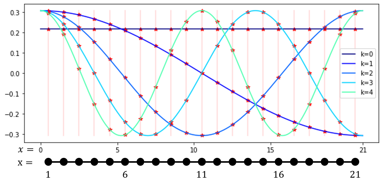
Now, we consider a special case of (2.2). In practice, the time-series model often contains a constant term, which is represented as a mode . In addition, it is usual to suppose that other modes are stationary and is -valued.


These conditions indicate a particular representation
| (2.8) |
where , and for and are distinct from each other. This form is also viewed as a general form of the inverse discrete Fourier transform (DFT), the modes of which are given by . See the difference of mode sets in Figure 2.1. As above, we assume that the amplitudes satisfy the non-degenerate condition
| (2.9) |
Then, as a special case of (2.4), we have the following lemma;
Lemma 2.10.
Take for . Then, satisfies
| (2.11) |
Proof..
For simplicity, set . Then, all satisfy
Now we have and because of the conditions for the mode set , as used in [16]. Hence, the above equation can be rewritten as
Therefore, by replacing by , we obtain the assertion. ∎
Remark 2.12.
For any mode set , the coefficients given in Lemma 2.10 satisfy and , as above. However, the converse is not always true. Namely, for the polynomial equation
when is a root, and become roots as well, where these two roots do not always coincide, as might be expected. For example, we can give a counterexample for .
The above lemma helps us to determine the modes from fewer observation points than Proposition 2.5, which needs observation points for model (2.11).
Proposition 2.13.
Proof..
For linear equation (2.6) for the coefficients , take and as asserted. Then, the matrix has rank because of non-degenerate condition (2.9). By using the argument in the proof of Lemma 2.10, we can transform that linear equation into the following equation for the coefficients :
| (2.14) |
Here, the matrix on the left still has rank , and then the coefficients and the modes are determined. ∎
2.3 Amplitude estimation
Once the modes in the general model (2.2) or the particular model (2.8) are obtained, the corresponding amplitudes are also calculated by the curve fitting method. For model (2.2), we have
| (2.15) |
for any . Since the Vandermonde matrix on the right has rank when , observed values at integer points determine all of the amplitudes .
Likewise, for model (2.8), we have
| (2.16) |
for any . Hence, the observed values at integer points determine all of the amplitudes . More generally, even for a dataset not generated from model (2.8), we can obtain this expansion. In other words, the following lemma holds.
Lemma 2.17.
Any real values are represented as
by distinct modes and , and . Moreover, and hold.
Proof..
Take -dimensional vectors
for . These vectors consist of a basis of because of the distinct condition. Then, we have their dual vectors such that , which are given by the inverse matrix of the matrix formed by . Therefore, is defined by for . Moreover, for , we have because is the dual vector of . ∎
In either case, the number of observation points needed to determine the amplitudes is less than that needed to determine the modes shown in Propositions 2.5 and 2.13. Therefore, the mode expansion techniques are summarized as follows:
Theorem 2.18.
We can use the estimated mode expansion for forecasting unobserved data.
Corollary 2.19.
When are determined from given observed points in Theorem 2.18, further values are computed for any .
2.4 Example
Here, let us consider the following time-series data for example;

| (2.20) |
for . See the plots in Figure 2.2.


By applying Proposition 2.5 for and to , we estimate modes and amplitudes, and then forecast the remaining values for . As is well known, Prony’s method is too sensitive to extract precise modes from numerical values, given as 64-bit floating point numbers in our case. Therefore, the results in Figure 2.3 show that the estimated modes are slightly different from the true values, and then such error accumulates to give a bad forecast.


On the other hand, Proposition 2.13 for and gives better results from a smaller number of values , as in Figure 2.4. This is because the absolute values of extracted modes are controlled to be , as explained in Figure 2.1.
In §4, we explain a more detailed algorithm with a graph recovery procedure.
3 Graph wave equation and graph recovery
In this section, we start from a review of the graph Laplacian and the graph wave equation from §3.1 to §3.3. In order to see an explicit solution of the graph wave equation, we calculate eigenfunctions for a path graph in §3.2, which is used in §4. Finally, we solve a graph recovery problem from the graph wave functions in §3.4.
3.1 Graph Laplacian
Let be graph weights that satisfy and for . In the present paper, we regard as a weighted undirected graph that has an edge - if and only if .
For a function , we define the graph Laplacian as
| (3.1) |
where . Note that graph weights are defined as a metric of -forms over a discrete set , and the graph Laplacian is given as the Laplace-Beltrami operator with an inner product [22]. Since the Laplacian is self-adjoint for this inner product, we can take eigenfunctions as follows:
| (3.2) |
Here, we see and for . Although the eigenfunctions have ambiguity regarding their signs even when the eigenvalues are distinct, we assume that the eigenfunctions are fixed in a certain manner. Moreover, in the present paper, we assume that a weighted graph is always connected, so that . The upper and lower bounds of the eigenvalues are well studied; for example, we have
| (3.3) |
The proof and other bounds of graphs are shown in [6].
3.2 Graph Fourier transform
Set for . Then, the eigenfunction expansion is given as
| (3.4) |
When the eigenvalues are distinct, this expansion is unique. In signal processing, the transformation is called the graph Fourier transform [13]. For the support function on , i.e., , we have . This calculation formally rewrites the eigenfunction decomposition of the graph Laplacian in (3.2) as the following identity concerning the graph weight:
| (3.5) |
Example 3.6 (Path graph).
Let us consider the path graph in Figure 3.1, which is defined by the weights
| (3.7) |

The eigenvalues and eigenfunctions are explicitly calculated as
| (3.8) |
for . This is directly checked via the identity
| (3.9) |
and so on. Here, as the upper bound (3.3), the largest eigenvalue satisfies . See also Figure 3.2 for . The corresponding graph Fourier transform is known as the discrete cosine transform in image processing [4].
Similarly, the graph Fourier transform for a cycle graph is known as the discrete Fourier transform (DFT) in signal processing and image processing [4].
3.3 Graph wave equation
By use of the graph Laplacian, we can define the following graph wave equation [11] for :
| (3.10) |
for a certain and given . For a solution , the graph Fourier coefficient becomes the harmonic oscillator
for ; hence, we can describe as
| (3.11) |
Therefore, graph wave equation (3.10) has a unique solution if and only if . For simplicity, we call this a graph wave function. In the present paper, we also assume that the Nyquist condition is satisfied:
| (3.12) |
This is always achieved by re-parameterizing by a higher sampling rate than , which also makes smaller, if necessary.
Here, it is worth noting that the above graph wave equation is naturally regarded as a discretization of the (continuous) wave equation
for , which is easily checked for the path graph . Namely, for the weights (3.7), the graph Laplacian gives the second-order central difference in the spatial domain
In order to see boundary conditions, we compare continuous and graph wave functions directly. The wave equation over with the Neumann conditions is written as
and its solution is explicitly described with some by
| (3.13) |

3.4 Graph recovery from graph wave function
The target in the present paper is to give a procedure to recover the graph weights from finite observed values at integer points . To state our main theorem, we simplify the representation of a graph wave function in (3.11) as
| (3.15) |
where , , and .
Theorem 3.16.
(i) Assume that the modes in (3.15) are distinct and unknown. If for all , then the modes , the eigenfunctions and the amplitudes are determined from observed valued at integer points .
(ii) The graph Laplacian and the graph weights are recovered from the given modes and the given eigenfunctions up to constant .
Proof..
In theory, the underlying graph is determined by Theorem 3.16. On the other hand, in numerical computation, it is often difficult to compute the underlying graph exactly because of numerical error, although we do not assume any noise. Therefore, in the following section, we summarize all of the above procedures as an algorithm.
4 Numerical experiments
In this section, we summarize the previous arguments into an algorithm, and then determine its performance using numerical datasets. In §4.1, we provide a six-step algorithm originating from Theorems 2.18 and 3.16. Then, in §4.2, §4.3, and §4.4, we apply the algorithm to graph wave signals, continuous wave signals, and human joint sensor time-series data, respectively.
4.1 Graph recover algorithm
For given multivariate wave signals, the number of variables is obviously known. Then, , , and in Proposition 2.13 and (2.16) should be optimal parameters to recover the underlying graph as the proof of Theorem 3.16. In addition, each calculated amplitude is supposed to be decomposed into and as . However, in practice, numerical error causes unexpected results in spite of Theorem 3.16. Therefore, we propose the following algorithm.
Algorithm 4.1.
Execute the following procedure:
- Step 1
-
Set such that , and take real values .
- Step 2
- Step 3
-
Obtain by solving the polynomial equation
(4.2) with the above , and compute so that for . Moreover, set and .
- Step 4
-
Get by solving linear equation (2.15) for with the above .
- Step 5
-
If a reconstructed is far from a validation dataset, then go back to Step 1 and retake larger and .
- Step 6
-
If is tiny, then set , otherwise . Then, define
(4.3) for any from the above . Optionally, we can retake this weight as instead if the graph weights are assumed to be non-negative.
Here, we present some remarks on this algorithm. For the graph recovery in Theorem 3.16, is supposed to be larger than as in examples §4.2 and §4.3. On the other hand, for a practical application, such as §4.4, smaller may work better to extract a significant graph. The condition means linear equation (2.14) is an overdetermined system. Hence, are computed by the least squares method or the pseudo-inverse matrix of the rectangular Vandermonde matrix. Then, modes are calculated as solutions of polynomial equation (4.2). For example, this part is practically computed as eigenvalues of the companion matrix of coefficients . As an expression of graph wave function (3.11), corresponds to the eigenvalue . If constant in graph wave equation (3.10) is known, then can be rescaled. Since the absolute value of is not always as explained in Remark 2.12, is sometimes retaken as . In either case, for , we have for a certain . Then linear equation (2.15) becomes (2.16). Hence, by Lemma 2.17, given values reconstruct a function as
| (4.4) |
for any . In an ideal case, is decomposed as by , and then the weights are estimated from identity (3.5). Instead, we set so that . Since is in in general, we replace by as in (4.3), in order to eliminate the ambiguity of an unit complex value on . Basically, this depends only on and up to the constant ; thus, partial observed values along are supposed to give a subgraph. We check this in §4.2.
Furthermore, we consider the meaning of the weight (4.3).


Since , the constant term in (4.4) does not affect the weights . The other term indicates the existence of the mode at node . Hence, when and have no common mode, they have no connection, i.e., . Moreover, when they are synchronized, becomes negative, and when they are anti-synchronized, becomes positive. To examine this property, let us consider the following example:
| (4.5) |
for . We have and , and then positivized weights are calculated as in Figure 4.1. There, the maximum value of the weights is .
4.2 Graph wave over an interval
We hereinafter demonstrate Algorithm 4.1 in order to verify its effectiveness. The first example is a graph wave function on an interval, as explained in §3.3. For and , let us take an initial function in the graph wave equation (3.10) over the path graph as
| (4.6) |
and .


Note that satisfy the assumption in Theorem 3.16, as in Figure 4.2. Moreover, we take so that even the largest eigenvalue satisfies Nyquist condition (3.12):
where upper bound (3.3) is used. Then, by applying the expression (3.11) to these conditions, we can see that the wave behavior becomes like the water in a bottle as in Figure 4.3. Although the function is continuous with respect to time variable as on the left-hand side, only integer points are used in the algorithm shown as the heat map on the right-hand side.

|

|
To this dataset, we apply Algorithm 4.1.


First, let us take and in Step 1. Then, we obtain modes from observation points along the time axis from Steps 2 and 3, as on the left-hand side in Figure 4.4. Note that although is larger than (the number of actual modes), such redundancy gives better results in numerical computation. Then, we obtain the corresponding amplitudes and weights from Steps 4 and 6. Since is given as above, can be used to calculate weights instead of in Step 6. On the right-hand side in Figure 4.4, we multiply the recovered weights by for visualization, which is quite close to the original weights in the path graph (3.7). Finally, we check the mean squared error in each as in Figure 4.5 to verify Step 5.

Since the error is tiny, even for test data, we conclude that the proposed graph recovery algorithm works well for this exact graph wave setting.
By modifying this dataset, let us consider another case when only partial observed values with respect to spatial variables are available.

For , assume the values on , and are missing. Then, a recovered graph is supposed to be the subgraph of the path graph in Figure 4.6.
To this dataset, we apply the same procedure as above, namely, take and , and then obtain modes . As the result on the left-hand side of Figure 4.7 shows, the extracted modes are basically the same as in the previous case, i.e., Figure 4.4. Then, the corresponding amplitudes and weights are also estimated, as on the right-hand side in Figure 4.7, which is close to what we expected in Figure 4.6.


These examples show that Algorithm 4.1 can correctly recover the underlying graph and subgraph from an observed graph wave function as Theorem 3.16 guarantees. In the following subsections, we consider other cases in which multivariate signals are not explicitly assumed to have a graph structure under variables.
4.3 Continuous wave over an interval
Unlike in §4.2, here we consider a continuous wave function on the interval explained in (3.13). Then, we apply Algorithm 4.1 to its observed values in expectation that the algorithm extracts a graph in the shape of an interval, although they do not satisfy the graph wave equation over a path graph.

|

|
Take in (3.13) as above. For an initial function , let us use a smoothened function of in (4.6). By using the identities
we define
In fact, these coefficients are nothing but the graph Fourier coefficients of , namely, for . Then, by the taking first coefficients and assuming , i.e., for any , we obtain a continuous wave function
| (4.7) |
for , which is shown in Figure 4.8. Here, we emphasize that this wave function is continuously defined for and , and thus there exist various ways to discretize it by evaluation. Moreover, the number is taken so that each frequency satisfies Nyquist condition (3.12), although this has another purpose, as explained below.
First of all, we evaluate the above at points along the -axis, for , and integer points along the time axis.


For these observed values, we take and in Step 1. Then, we obtain modes from observation points from Steps 2 and 3, as on the left-hand side in Figure 4.9, and the corresponding amplitudes and weights from Steps 4 and 6, as on the right-hand side.

The estimated weights indicate the path-like graph at the top of Figure 4.10, which includes the path graph below. Thus, the same procedure for a partial observed dataset like in Figure 4.6 is applicable to obtain the path graph.


Namely, we try another discretization for , given on the left-hand side in Figure 4.11. Then, by using the same parameter, we successfully obtain the weights close to those of the path graph on the right-hand side in Figure 4.11 expected from the bottom path graph in Figure 4.10.
This phenomenon can be explained in another way. From observed values , a matrix formed by is constructed as in linear equation (2.14) in Step 2.

Here, we can see that the matrix has rank , which means its singular values consist of major values and minor values, as in Figure 4.12. This is consistent with the definition of , where we take the terms in the summation other than the constant term (4.7). Hence, it is sufficient to use more than observation points, such as observed values as above, in order to extract an outline of the underlying graph.
4.4 Pose model
As a more practical case, we consider a graph estimation problem from human joint tracking data. To this end, we use an open source dataset PKU-MMD, which consists of RGB, skeletons, depth, and IR sequential data for 51 action categories [7]. The skeleton data we use herein are obtained by Kinect v2, the joints of which are described as in Figure 4.13 [1]. More strictly speaking, we use the 2,100th to 2,800th frames from the "0007-M" sample in the dataset.

|

|
Although the skeleton data provide the three-dimensional coordinates , , and of each joint location in space, we only use the and coordinates in this experiment. Then, we try to extract relations among moving joint locations as graphs, which are supposed to characterize individual actions.
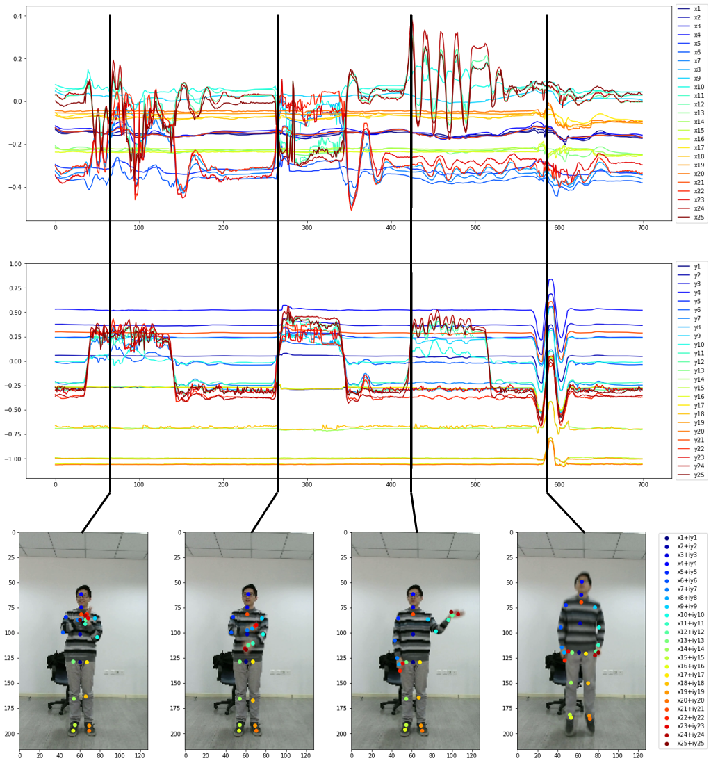
Let and denote functions of the and locations in an RGB image, respectively, for the joint nodes and the times . First, as time series, we apply Steps 1 to 5 of Algorithm 4.1 for and to a -long sequence starting from the -th frame. Then, we obtain mode decompositions
| (4.8) |
for any node so as to coincide with and on the sequence . See also Lemma 2.17. Here, we can see that represents the time evolution of the location in an RGB image. Finally, we calculate (4.3) for in order to estimate weights among joint locations at . Note that although and no longer satisfy the graph wave equation for the estimated graph, we suppose that the graph weights extract meaningful features from the decomposition (4.8).
For example, we pick out four sequences representing "clapping" from the 2,165th to 2,180th frames (), "cross hands in front" from the 2,365th to 2,380th frames (), "hand waving" from the 2,525th to 2,540th frames (), and "jump up" from the 2,685th to 2,700th frames (). The corresponding data are shown in Figure 4.14. Then, we draw the resulting graphs in Figure 4.15, where each edge indicates that the estimated weight is larger than .

As we can see, edges in each case are illustrated on nodes and pairs that characterize each action. In particular, since we are paying attention to positive weights, Algorithm 4.1 ignores synchronized pairs and extracts anti-synchronized pairs. Hence, even in the "jump up" case, only the leg motion is highlighted against all upward moving nodes. As in this case, we expect that the proposed graph recovery algorithm will work well, even for non-wave signals.
5 Conclusion
In the present paper, we introduced a graph recovery method from a graph wave function based on a modified DMD algorithm. Then, we showed its effectiveness by using three examples, i.e., a graph wave function, a continuous wave function, and human joint tracking data, from viewpoints of from theoretical demonstration to practical study. In the present study, we do not assume the existence of noise in each time-series model. Hence, further study is needed in order to assure that the proposed algorithm works against noises, such as white noise, with the help of known technologies in signal processing, time-series analysis, and statistics.
Acknowledgements
The author would like to thank Yosuke Otsubo for discussing and suggesting DMD technology for further study. The author is also grateful to Satoshi Takahashi, Tetsuya Koike, Chikara Nakamura, Bausan Yuan, Ping-Wei Chang, and Pranav Gundewar for their constant encouragement.
References
- [1] Kinect for windows v2 referece, jointtype enumeration. https://docs.microsoft.com/en-us/previous-versions/windows/kinect/dn758662(v=ieb.10).
- [2] Amaia Abanda, Usue Mori, and Jose A Lozano. A review on distance based time series classification. Data Mining and Knowledge Discovery, 33(2):378–412, 2019.
- [3] Faisal Ahmed, Padma Polash Paul, and Marina L Gavrilova. Dtw-based kernel and rank-level fusion for 3d gait recognition using kinect. The Visual Computer, 31(6):915–924, 2015.
- [4] Rosa A Asmara and Reza Agustina. Comparison of discrete cosine transforms (dct), discrete fourier transforms (dft), and discrete wavelet transforms (dwt) in digital image watermarking. International Journal of Advanced Computer Science and Applications, 8(2):245–249, 2017.
- [5] Donald J Berndt and James Clifford. Using dynamic time warping to find patterns in time series. In KDD workshop, volume 10, pages 359–370. Seattle, WA, USA:, 1994.
- [6] Fan RK Chung and Fan Chung Graham. Spectral graph theory. Number 92. American Mathematical Soc., 1997.
- [7] Liu Chunhui, Hu Yueyu, Li Yanghao, Song Sijie, and Liu Jiaying. Pku-mmd: A large scale benchmark for continuous multi-modal human action understanding. arXiv preprint arXiv:1703.07475, 2017.
- [8] Sacha Epskamp, Lourens J Waldorp, René Mõttus, and Denny Borsboom. The gaussian graphical model in cross-sectional and time-series data. Multivariate behavioral research, 53(4):453–480, 2018.
- [9] Christos Faloutsos, Mudumbai Ranganathan, and Yannis Manolopoulos. Fast subsequence matching in time-series databases. ACM Sigmod Record, 23(2):419–429, 1994.
- [10] George E Forsythe. Generation and use of orthogonal polynomials for data-fitting with a digital computer. Journal of the Society for Industrial and Applied Mathematics, 5(2):74–88, 1957.
- [11] Joel Friedman and Jean-Pierre Tillich. Wave equations for graphs and the edge-based laplacian. Pacific Journal of Mathematics, 216(2):229–266, 2004.
- [12] Paolo Giudici and Alessandro Spelta. Graphical network models for international financial flows. Journal of Business & Economic Statistics, 34(1):128–138, 2016.
- [13] David K Hammond, Pierre Vandergheynst, and Rémi Gribonval. Wavelets on graphs via spectral graph theory. Applied and Computational Harmonic Analysis, 30(2):129–150, 2011.
- [14] Meng Li and Howard Leung. Graph-based approach for 3d human skeletal action recognition. Pattern Recognition Letters, 87:195–202, 2017.
- [15] Ta-Hsin Li. Time series with mixed spectra. CRC Press, 2013.
- [16] Ta-Hsin Li and Benjamin Kedem. Asymptotic analysis of a multiple frequency estimation method. Journal of multivariate analysis, 46(2):214–236, 1993.
- [17] Gerlind Plonka and Manfred Tasche. Prony methods for recovery of structured functions. GAMM-Mitteilungen, 37(2):239–258, 2014.
- [18] Ivan Popivanov and Renee J Miller. Similarity search over time-series data using wavelets. In Proceedings 18th international conference on data engineering, pages 212–221. IEEE, 2002.
- [19] R Prony. Essai experimental et analytique. Journal de L’Ecole Polytechnique, 1(2):24–76, 1795.
- [20] Peter J Schmid. Dynamic mode decomposition of numerical and experimental data. Journal of fluid mechanics, 656:5–28, 2010.
- [21] Kilian Stampfer and Gerlind Plonka. The generalized operator based prony method. Constructive Approximation, 52(2):247–282, 2020.
- [22] Yuuya Takayama. Geometric formulation for discrete points and its applications. arXiv preprint arXiv:2002.03767, 2020.
- [23] Jeff KT Tang and Howard Leung. Retrieval of logically relevant 3d human motions by adaptive feature selection with graded relevance feedback. Pattern Recognition Letters, 33(4):420–430, 2012.
- [24] Jonathan H Tu. Dynamic mode decomposition: Theory and applications. PhD thesis, Princeton University, 2013.
- [25] Caroline Uhler. Gaussian graphical models: An algebraic and geometric perspective. arXiv preprint arXiv:1707.04345, 2017.
- [26] Ting Wang, Zhao Ren, Ying Ding, Zhou Fang, Zhe Sun, Matthew L MacDonald, Robert A Sweet, Jieru Wang, and Wei Chen. Fastggm: an efficient algorithm for the inference of gaussian graphical model in biological networks. PLoS computational biology, 12(2):e1004755, 2016.