Graph Perceiver IO: A General Architecture for Graph Structured Data
2Chung-Ang University
)
Abstract
Multimodal machine learning has been widely studied for the development of general intelligence. Recently, the remarkable multimodal algorithms, the Perceiver and Perceiver IO, show competitive results for diverse dataset domains and tasks. However, recent works, Perceiver and Perceiver IO, have focused on heterogeneous modalities, including image, text, and speech, and there are few research works for graph structured datasets. A graph is one of the most generalized dataset structures, and we can represent the other dataset, including images, text, and speech, as graph structured data. A graph has an adjacency matrix different from other dataset domains such as text and image, and it is not trivial to handle the topological information, relational information, and canonical positional information. In this study, we provide a Graph Perceiver IO, the Perceiver IO for the graph structured dataset. We keep the main structure of the Graph Perceiver IO as the Perceiver IO because the Perceiver IO already handles the diverse dataset well, except for the graph structured dataset. The Graph Perceiver IO is a general method, and it can handle diverse datasets such as graph structured data as well as text and images. Comparing the graph neural networks, the Graph Perceiver IO requires a lower complexity, and it can incorporate the local and global information efficiently. We show that Graph Perceiver IO shows competitive results for diverse graph-related tasks, including node classification, graph classification, and link prediction.
1 Introduction
Humans who have general intelligence has the capability to handle multiple datasets from different source simultaneously. One of the required building blocks for general intelligence is multimodal learning for a general perception, and there has been much interest in multimodal learning. With the development of the Transformer [1] and the Vision Transformer (ViT) [2], there have been multimodal learning approaches that adopts multiple Transformer encoders for each modality [3, 4], and fuses the each information later [5].
Another remarkable algorithms for multimodal learning are the Perceiver [6] and its extension, the Perceiver IO [7], general architecture that has structured inputs and outputs. Perceiver IO handles various sizes of inputs and outputs, and they unify the inputs and outputs structures for diverse types of datasets such as images and text. Unified inputs and outputs structures make the single model, Perceiver IO, handle multimodal datasets simultaneously. With Perceiver IO, the specific neural networks for each modality are not required.
There have been some research works for multimodal learning, and most works have focused on images, text, and speech instead of graph structured data. A graph has topological information. The topological information can be divided by relational information and canonical positional information. Especially, the relational information, described as an adjacency matrix, is a distinct features different from the other dataset. The Perceiver and Perceiver IO flatten all inputs, and they adopt the positional encodings to describe the spatial information or the sequence order. However, a graph has no such sequence order, and it has explicit relationships different from other datasets. Besides, the proper input and output query array structure for multiple graph-related tasks has not been explored yet.
Parallel to multimodal learning, there have been many works for the graph structured dataset. A graph has a node and topological information, and a graph is known to be a general type that can represent diverse types of the dataset, including image and text [8]. From its general property, the graph has diverse application areas such as knowledge graph completion [9, 10], drug discovery [11, 12] and social network analysis [13, 14]. The graph has meaningful knowledge information, and the intelligence learned from a graph structured dataset might be important for general intelligence as well as other datasets.
In this paper, we propose the Graph Perceiver IO, a general method to handle the graph structured dataset as well as diverse modality. The Graph Perceiver IO takes the raw node features and graph positional encoding to reflect node features and to distinguish various shape of graphs, canonical positional information. Besides, The Graph Perceiver IO can handle relational information of graph through smoothing based output query array design. For the Graph Perceiver IO, we keep the model structure of Perceiver IO as much as possible because it is already a general architecture for multimodal datasets except graph neural networks. The Graph Perceiver IO has two advantages over the traditional GNNs. First, the Graph Perceiver IO has a lower space complexity. For the given input array, latent array, and output query array, the computation of Perceiver IO does not depend on an adjacency matrix. While the complexity of traditional GNNs is proportional to the squared number of nodes, the Graph Perceiver IO has linear complexity. Second, the Graph Perceiver IO handles both global structure and local structure information. The Graph Perceiver IO does not have a restriction on the attention areas, and all nodes can interact with attention. It is noted that the locality inductive bias can be injected into the Graph Perceiver IO with the positional encoding and output query. Third, the Graph Perceiver IO can handle multimodal data, including the graph, simultaneously. The single unified model, the Graph Perceiver IO, is necessary to consider the multimodal data such as image and graph, while the traditional methods need two networks for image and graph, respectively.
2 Related Works
2.1 Multimodal Learning
Multimodal machine learning addresses fundamental goals for artificial intelligence by integrating and modeling multiple modalities, including visual, linguistic, and acoustic signals. Here, we introduce two branches of multimodal research: representation learning and general architecture.
Multimodal representation learning
Based on a tremendous amount of image-text pair datasets, contrastive pre-trained multimodal models such as CLIP [3] and Align [15] recently show impressive progress w.r.t generalizability of representation and zero-shot transfer. A key factor to their great success is the language-guided visual representation learning scheme. Given a set of image-caption pairs , they train an image encoder and text encoder such that the similarity between positively aligned pair is maximized relative to negatively unaligned pair through InfoNCE [16] objective function. In addition to image-text learning, video-text learning [17], [18], and speech-text learning [19], [20] have also studied actively.
General architecture
In another line of work, there are attempts that aim to unify the architecture or learning objective for training in different modalities. Most of these studies mainly utilize the Transformer [1] architecture which has less data-specific and task-specific inductive bias as the backbone. Instead of relying on modality-specific targets, Data2vec [21] uses the same learning objective for data from different modalities. Based on the combination objective of latent target prediction task [22], [23] and Masked prediction [24], [25], Data2vec shows promising results on three different modalities including text, image and speech.[6] propose a general framework Perceiver to handle arbitrary configurations of different modalities. Without making domain-specific assumptions, Perceiver encodes the data point through iterative self-attention and cross-attention. And they mitigate the quadratic scaling problem of self-attention blocks in Transformer by processing a small set of latent units instead of high-dimensional inputs. Recently, Perceiver IO [7] appeared to extend the capable task that the original Perceiver can not perform, and Hierarchical Perceiver [26] improves the performance and efficiency of the Perceiver by introducing locality into the model architecture while preserving its modality-independence property. Our proposed model, Graph Perceiver IO, further extends the accommodatable modality of Perceiver IO to the graph structured dataset.
2.2 Graph Structured Modeling
Graph Neural Networks (GNN) is an efficient and well-designed framework for geometric data. The use of GNNs has expanded the range of applications for frameworks based on neural networks.
Graph Neural Networks
The representative method of Graph Neural Networks (GNN) is GCN [27] which provides spatial domain graph convolution by approximating a spectral graph convolution. GCN propagates a node representation by using a normalized adjacency matrix. APPNP proposes a way of propagation based on personalized PageRank, which is one of the GCN variants. The message passing based models like GCN, GAT [28], GrpahSAGE [29], etc., have improved classification ability on node-level and graph-level tasks. Furthermore, various modified models of GNNs in link prediction tasks ensure reliable performance. [30] predict a link using an inner product between the latent embeddings of target nodes encoded based on a variational autoencoder [31, 32]. [33] propose VGNAE that applies -normalization before propagation to alleviate the issue that an isolated node embed got close to zero by VGAE [30]. There are recent works of Graph Transformer that utilizes the transformer to the graph structured dataset. The expression of relational information how to redefine a positional encoding and how to learn representations using relational information. [34, 35, 36]
3 Preliminary
Our proposed model, Graph Perceiver IO, is based on the Perceiver IO, a general architecture with flexible input and outputs. In this section, we introduce the Perceiver and the Perceiver IO in detail.
3.1 Perceiver
Jaegle et al. [6] proposes the Perceiver, a general perception module with iterative attention for handling the diverse and high-dimensional multimodal inputs. The Perceiver has two components of arrays, input arrays , and latent arrays . For given data instances, the Perceiver transforms the given data instances as the inputs array where and denote the dataset properties such as the image size and the number of channels. The latent arrays are learnable latent representations, where and are the number of latent and the latent dimension, respectively. The Perceiver adopts the two types of attention, cross-attention and self-attention, and both attentions are query-key-value attention, similar to the Transformer [1]. First, the cross-attention computes the attention between the latent arrays and the input arrays. The latent arrays are queries, and they attend to the important information from the key, the input arrays. The relevant input features for the given tasks are incorporated into the latent array with cross-attention. Second, the Perceiver adopts the self-attention for the latent arrays. Attention between latent arrays and input arrays reduces the time and space complexity compared to the self-attention for the input arrays only. The attention complexity of the Perceiver is while the complexity of the self-attention for input-image is . In summary, the Perceiver is composed of the multiple blocks of cross-attention and the latent Transformer that adopts the self-attention for the latent arrays. The input arrays are fed into the Transformer iteratively across the layers. After the multiple blocks, the Perceiver adopts the average pooling over the index dimension and utilizes it to predict the target label.
3.2 Perceiver IO
The Perceiver is a general model that handles diverse datasets with flexible input structures. However, the output structure of the Perceiver is not flexible, and the Perceiver is limited to the classification tasks. To extend the Perceiver into diverse tasks such as language modeling and autoencoding, flexible output structures are necessary. Perceiver IO proposes an additional output query array components for the flexible outputs structure. For the image classification task, the and denote the number of images and the number of classes, respectively. Perceiver IO adds the additional query-key-value attention block on the top of the Perceiver. The additional attention block computes the attention between the output query array and the latent arrays extracted by the Perceiver. The shape of the output query array is a controllable hyper-parameter, and it induces flexible output structures that produce any size of outputs.
The Perceiver and Perceiver IO attend to the relationship between the latent arrays and input arrays. They adopt query-key-value attention that is similar to the Transformer. Different from the convolutional neural nets (CNN) [37, 38] or the vision Transformer (ViT) [39, 40], the Perceiver operates on the individual pixels independently without patches or convolution operations. However, attention computation is permutation invariant, and the attention-only mechanism is hard to treat the sequence order. To incorporate the order information for sequence and spatial information for images, the Perceiver and the Perceiver IO introduce the learned positional encoding or Fourier-based positional encoding with sinusoid functions.

3.3 Perceiver IO and Graph Structured Data
The Perceiver is a general architecture, and it has high flexibility for input and output structure. From its flexibility and generality, The Perceiver and its variants
handle the diverse tasks for image, text, speech, and 3D point clouds. They extend their works to incorporate the heterogeneous multimodal dataset such as audiovisual sequences, and the Perceiver shows competitive results. However, the application of Perceiver is limited to the non-graph structured dataset, and they do not handle the graph structured dataset that has topological information.
Extending the Perceiver to handle the graph structured dataset is non-trivial. First, the Perceiver is a general architecture, and it already shows the competitive results for diverse tasks. Therefore, simple extensions that do not modify the overall model structures are required. Second, the Perceiver receives the flattened inputs, and incorporating the topological information represented by the adjacency matrix into the Perceiver is challenging.
4 Methodology
4.1 Overall Structure
Graph data usually consists of matrix, a set of nodes features, and adjacency matrix , which represents a set of relational information between nodes. In order to train graphs using Perceiver IO, the input array and the output query array should be constructed by using and properly. To handle the graph-structured data, topological information is essential. We can divide the topological information on the graph as relational information and canonical positional information. Both two information is essential for the graph-related tasks such as node classification and graph classification. To incorporate the topological information, we propose the following two methods 1) output query smoothing, and 2) positional embedding as shown in the Figure 1. The shape of the output query array depends on the given task, and we will discuss it in Section Output Query Array. The overall structure of our proposed model is in Figure 2.
4.2 Output Query Array
One of the major problems of the Graph Perceiver IO is to incorporate the adjacency matrix. The adjacency matrix that is widely utilized in GNNs is not adaptable for the Graph Perceiver IO. Also, the Graph Perceiver IO requires a flexible output structure to handle the diverse graph-related tasks such as node classification, graph classification, and link prediction. For the flexible output array structure, we adopt the output query array by following the Perceiver IO. The output query shape can be determined by the task specifically. It is noted that the output query can be used as a pretrained embedding, or it can be learnable parameters. For graph classification task that requires a single label per graph, we set the output query size as , where denotes the output query array dimension. For node-specific tasks such as node classification and link prediction, we set the output array shape as where is the number of nodes. The simple choice of the output array is raw nodes features that is the same as the input array. However, we find that the output query array based on the raw node features tends to show poor performance. Furthermore, raw node features do not contain any relational information of adjacency matrix. Instead of raw node features, we propose a smoothing based output query array that is smoothed features of raw node features times [41]. The following Eq. 1 denotes the times smoothed node features, the output query array of the Graph Perceiver IO,
| (1) |
where denotes a adjacency matrix with self-loop and denotes node degree matrix of . SGC [41] removes nonlinear function between GCN layers and collapse repeated multiplication of matrix into -th power of matrix like Eq. 1 which extracts smoothed features of . As a result, extracted features tends to have similar representation to nearby nodes and help to make similar predictions. That is, the SGC incorporates adjacency matrix into its input to get -hops neighbor information. In a similar way, we utilize adjacency matrix to obtain as an output query array which contain relational information.
Besides, we adopt the APPNP smoothing [42] as an output query array as shown in Eq. 4.2.
| (2) |
APPNP adopts personalized propagation, and it provides more data specific smoothing methods. We empirically find that the output query with a smoothing method is one of the key factors for the Graph Perceiver IO.

4.3 Input Array
The Graph Perceiver IO requires the same input structure as the Perceiver or Perceiver IO. For image and text dataset, jaegle et al. propose Fourier embedding to consider the spatial or sequential information, but it shows poor performance for graph classification [7]. Appendix C. presents a detailed result. To reflect the topological information, specifically canonical positional information, with the original Perceiver input array structure, we adopt the random walk positional embedding () [43]. Random walk operators are defined as where is the adjacency matrix, and is the degree matrix. of node is defined as
| (3) |
where is the probability of starting from the node, walking times, and returning to the node. dwivedi et al. adopt as positional encoding initialization for distinguishing several cases of non-isomorphic graphs and structurally different nodes which messeage-passing GNNs and 1-WL fail to distinguish. The choice of sufficiently large gives a unique node representation to distinguish each node and graph. Besides the node features, we concatenate the to obtain nodes representation distinguishing non-isomorphic graphs and structurally different nodes. There is no restriction on the attention coverage, and it makes the Graph Perceiver IO handles the global structure information efficiently. It is noted that the injection of into the Graph Perceiver can be interpreted as an inductive bias to consider the local information as well as the global information. Compared to typical GNNs, the Perceiver has lower space complexity in terms of the input array. GNNs requires on dense graph, while the Perceiver Graph IO needs , where is the controllable hyper-parameters.
4.4 Graph Related Tasks
The Graph Perceiver IO has the capability to perform diverse graph-related tasks such as classification and prediction. In node classification tasks, the output array obtained after going through the logits layer contains each node’s predicted score. We use the cross-entropy loss to learn node embedding. For graph classification tasks, we set a size of output query array to 1-dimension vector. Then we pass the array to the logits layer (e.g., a single linear layer) instead of the read-out layer usually used for global pooling in graph-level tasks. We evaluate the cross-entropy loss with target label.
For link prediction tasks, we conduct the inner product between each pair of node features which is the output of the last cross attention layer. In the same manner, as GAE [30], We use the reconstruction loss for training our model. Table 1 provides configuration of each array and whether or not the logits layer is used for each task.
| Tasks | input array | Output query array | Logits layer |
|---|---|---|---|
| Node classification | O | ||
| Graph classification | O | ||
| Link prediction | X |
4.5 Complexity Analysis
The Graph Perceiver IO requires a single adjacency matrix-related operation to make the smoothed output query before the model training. The smoothing operation is only once conducted, and it never appears during the model training. The mechanism is similar to the Simplifying Graph Convolutional (SGC) [41] that only performs single adjacency matrix-related operation. Therefore, the Graph Perceiver IO has an efficient computation time compared to the other graph neural networks. Besides, there is no attention between inputs, but there is attention between the latent array and the input array, or the output query array and the input array. The complexity of attention between latent arrays does not depend on the number of nodes, and the complexity of attention between latent and input arrays depends on the number of nodes linearly. However, the current Transformer variants, such as Graph Transformer architecture [34] adopt the input-wise attention, and the computation time is proportional to the square of a number of nodes. Therefore, Graph Perceiver IO has advantages in the time complexity as well as its simplicity and multi-modal learning.
5 Results
To validate our proposed model, the Graph Perceiver IO, we conduct comprehensive experiments, node classification, graph classification, and link prediction. Appendix B. provides the more detailed experimental settings.
5.1 Dataset
We provide comprehensive experimental resists for diverse datasets and tasks. Table 2 describes the dataset statistics for graph-related tasks. For the preprocessing and train/test splits, we follow the benchmark experimental settings for each task and dataset. We follow the same settings with the [44] for node classification, graph classification and link prediction, respectively. We provide the dataset as well as the source code as supplementary files. It is noted that the graph-related dataset will be downloaded automatically upon running the source code.
| Dataset | Graphs | Nodes | Edges | Features | Classes |
| Cora | 1 | 2,708 | 5,278 | 1,433 | 7 |
| CiteSeer | 1 | 3,327 | 4,552 | 3,703 | 6 |
| PubMed | 1 | 19,717 | 44,324 | 500 | 3 |
| MUTAG | 188 | 17.93 | 19.79 | 7 | 2 |
| PROTEINS | 1,113 | 39.06 | 72.82 | 3 | 2 |
| IMDB-BINARY | 1,000 | 19.77 | 96.53 | - | 2 |
| REDDIT-BINARY | 2,00 | 429.63 | 497.754 | - | 2 |
| COLLAB | 5,000 | 74.49 | 2,457.22 | - | 3 |
5.2 Node Classification
For node classification experiments, we adopt the three benchmark data, Cora [45], CiteSeer [46], and PubMed [47]. We follow all experimental settings from [44], and we repeat the experiment 100 times. Table 3 denotes the accuracy of node classification task. The Graph Perceiver IO shows relatively lower results compared to the advanced graph neural networks, but our model shows the competitive results on the PubMed dataset.
| Model | Cora | CiteSeer | PubMed | |||
|---|---|---|---|---|---|---|
| Fixed | Random | Fixed | Random | Fixed | Random | |
| GCN [27] | 81.4 | 78.7 | 71.1 | 68.1 | 78.9 | 77.3 |
| GAT [28] | 83.0 | 80.9 | 70.9 | 68.8 | 78.9 | 77.6 |
| Cheb [48] | 80.5 | 77.0 | 69.8 | 67.2 | 78.2 | 75.4 |
| SGC [41] | 81.7 | 80.1 | 71.3 | 68.5 | 78.9 | 76.6 |
| ARMA [49] | 82.2 | 79.8 | 71.0 | 67.9 | 78.8 | 77.6 |
| APPNP [42] | 83.3 | 82.1 | 71.7 | 69.8 | 80.1 | 79.1 |
| Graph Perceiver IO | 83.9 | 81.6 | 70.1 | 68.1 | 79.9 | 79.6 |

To analyze the attention properties of the Graph Perceiver IO, we visualize the attention weights of cross-attention and the attention between the latent arrays and the input arrays as shown in Figure 3. Each latent index in the Graph Perceiver IO captures the different nodes with high diversity. Additionally, each latent focuses on the specific class group of nodes relatively. Besides, we analyze the learned embedding from the Graph Perceiver IO as shown in Figure 4. From the embedding visualization, we validate the Graph Perceiver IO has a relatively high uniformity embedding space.


5.3 Link Prediction
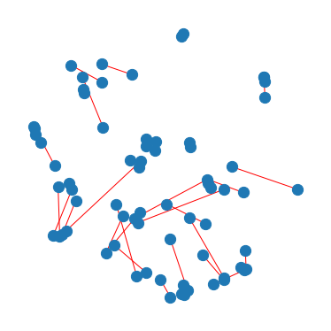
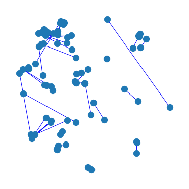
Besides the classification task, we validate our models on the link prediction task. Table 4 denotes the results of the link prediction task. We utilize the features extracted by the cross attention between the output query array and latent array for the link prediction task. The Graph Perceiver IO shows the competitive results with the VGAE [30], but our model shows competitive performance compared to the state-of-the-art, VGNAE [33], that utilizes the additional normalization steps with the VGAE. It denotes that incorporating the further graph-specific regularization term into Graph Perceiver IO would be necessary. In Figure 5, we plot t-SNE to compare the performance of the three models in link prediction task.
| Model | Cora | CiteSeer | PubMed | |||
|---|---|---|---|---|---|---|
| AUC | AP | AUC | AP | AUC | AP | |
| Spectral Clustering [52]* | 84.6 | 88.5 | 80.5 | 85.0 | 84.2 | 87.8 |
| DeepWalk [53]* | 83.1 | 85.0 | 80.5 | 83.6 | 84.4 | 84.1 |
| DGI [54]* | 89.8 | 89.7 | 95.5 | 95.7 | 91.2 | 92.2 |
| ARGVA [55]* | 92.4 | 93.2 | 92.4 | 93.0 | 96.8 | 97.1 |
| GIC [56] | 90.0 | 89.9 | 95.8 | 95.8 | 90.9 | 91.6 |
| VGAE [30] | 95.2 | 94.7 | 92.0 | 91.6 | 95.6 | 95.3 |
| GNAE [33] | 95.6 | 96.0 | 97.2 | 97.3 | 97.7 | 97.6 |
| VGNAE [33] | 95.8 | 95.7 | 96.8 | 96.7 | 97.3 | 97.2 |
| Graph Perceiver IO | 95.9 | 96.4 | 96.8 | 97.2 | 97.6 | 97.8 |


5.4 Graph Classification
| Model | MUTAG | PROTEINS |
|
|
COLLAB | ||||
|---|---|---|---|---|---|---|---|---|---|
| GCNWithJK | 72.9 | 72.6 | 73.2 | 89.4 | 81.5 | ||||
| SAGPool | 74.0 | 72.3 | 72.3 | 89.0 | 78.9 | ||||
| DiffPool | 84.6 | 74.3 | 74.8 | 92.7 | 79.4 | ||||
| EdgePool | 72.3 | 72.6 | 73.3 | 89.2 | 79.3 | ||||
| GCN | 70.7 | 72.2 | 74.2 | 89.1 | 81.0 | ||||
| GraphSAGE | 75.1 | 74.1 | 73.2 | 90.7 | 79.8 | ||||
| GIN0 | 81.9 | 73.1 | 73.7 | 90.9 | 80.5 | ||||
| GIN | 82.9 | 72.0 | 73.5 | 90.5 | 80.7 | ||||
| GlobalAttentionNet | 77.7 | 72.6 | 72.9 | 88.6 | 79.1 | ||||
| Set2SetNet | 74.5 | 74.1 | 72.7 | 90.3 | 79.4 | ||||
| SortPool | 83.0 | 73.9 | 71.8 | 84.3 | 77.8 | ||||
| ASAP | 78.7 | 74.0 | 72.2 | OOM | 79.4 | ||||
| Graph Perceiver IO | 86.1 | 76.1 | 72.9 | 91.6 | 79.1 |
We validate our models on the graph classification task. Graph classification tasks require the understanding of both the local and global graph structures. We repeat the experiments ten times, and we follow the same experimental protocols with the [44]. Table 5 denotes the accuracy of the graph classification on diverse benchmark dataset. For MUTAG [57] and PROTEINS [57], Graph Perceiver IO shows superior performance compared to the recent GNNs. In short, Graph Perceiver IO has a high capacity to incorporate both the node features and link information simultaneously. It is noted that MUTAG and PROTEINS have node features while IMDB, REDDIT, and COLLAB [58] have no node features. Even though there are no node features, the Graph Perceiver IO has competitive results with the recent GNNs. It denotes that the Graph Perceiver IO handles the topological information of graph structured data with the positional embeddings.
6 Conclusion
Multimodal learning graph structured dataset, as well as text, image, and speech, is necessary for general perception. In this paper, we propose Graph Perceiver IO that handles the graph structured dataset as well as other datset such as image and text. Graph Perceiver IO provides the competitive results for the representative graph-related tasks. Graph Perceiver IO handles topological information, relational information and canonical positional information. It can incorporate the global and local information with a lower complexity compared to the traditional graph neural networks. Overall, Graph Perceiver IO is a general architecture for handling diverse modalities and tasks, including graph-related works. We will leave the diverse multimodal learning task such as image-text-graph and visual question answering with knowledge graph as the future works.
References
- [1] Ashish Vaswani, Noam Shazeer, Niki Parmar, Jakob Uszkoreit, Llion Jones, Aidan N Gomez, Łukasz Kaiser, and Illia Polosukhin. Attention is all you need. Advances in neural information processing systems, 30, 2017.
- [2] Alexey Dosovitskiy, Lucas Beyer, Alexander Kolesnikov, Dirk Weissenborn, Xiaohua Zhai, Thomas Unterthiner, Mostafa Dehghani, Matthias Minderer, Georg Heigold, Sylvain Gelly, Jakob Uszkoreit, and Neil Houlsby. An image is worth 16x16 words: Transformers for image recognition at scale. In International Conference on Learning Representations, 2021.
- [3] Alec Radford, Jong Wook Kim, Chris Hallacy, Aditya Ramesh, Gabriel Goh, Sandhini Agarwal, Girish Sastry, Amanda Askell, Pamela Mishkin, Jack Clark, et al. Learning transferable visual models from natural language supervision. In International Conference on Machine Learning, pages 8748–8763. PMLR, 2021.
- [4] Soravit Changpinyo, Piyush Sharma, Nan Ding, and Radu Soricut. Conceptual 12m: Pushing web-scale image-text pre-training to recognize long-tail visual concepts. In Proceedings of the IEEE/CVF Conference on Computer Vision and Pattern Recognition, pages 3558–3568, 2021.
- [5] Junnan Li, Ramprasaath Selvaraju, Akhilesh Gotmare, Shafiq Joty, Caiming Xiong, and Steven Chu Hong Hoi. Align before fuse: Vision and language representation learning with momentum distillation. Advances in Neural Information Processing Systems, 34, 2021.
- [6] Andrew Jaegle, Felix Gimeno, Andy Brock, Oriol Vinyals, Andrew Zisserman, and Joao Carreira. Perceiver: General perception with iterative attention. In International Conference on Machine Learning, pages 4651–4664. PMLR, 2021.
- [7] Andrew Jaegle, Sebastian Borgeaud, Jean-Baptiste Alayrac, Carl Doersch, Catalin Ionescu, David Ding, Skanda Koppula, Daniel Zoran, Andrew Brock, Evan Shelhamer, Olivier J Henaff, Matthew Botvinick, Andrew Zisserman, Oriol Vinyals, and Joao Carreira. Perceiver IO: A general architecture for structured inputs & outputs. In International Conference on Learning Representations, 2022.
- [8] Peter W Battaglia, Jessica B Hamrick, Victor Bapst, Alvaro Sanchez-Gonzalez, Vinicius Zambaldi, Mateusz Malinowski, Andrea Tacchetti, David Raposo, Adam Santoro, Ryan Faulkner, et al. Relational inductive biases, deep learning, and graph networks. arXiv preprint arXiv:1806.01261, 2018.
- [9] Quan Wang, Zhendong Mao, Bin Wang, and Li Guo. Knowledge graph embedding: A survey of approaches and applications. IEEE Transactions on Knowledge and Data Engineering, 29(12):2724–2743, 2017.
- [10] Zhao Zhang, Fuzhen Zhuang, Hengshu Zhu, Zhiping Shi, Hui Xiong, and Qing He. Relational graph neural network with hierarchical attention for knowledge graph completion. In Proceedings of the AAAI Conference on Artificial Intelligence, volume 34, pages 9612–9619, 2020.
- [11] Zhaoping Xiong, Dingyan Wang, Xiaohong Liu, Feisheng Zhong, Xiaozhe Wan, Xutong Li, Zhaojun Li, Xiaomin Luo, Kaixian Chen, Hualiang Jiang, et al. Pushing the boundaries of molecular representation for drug discovery with the graph attention mechanism. Journal of medicinal chemistry, 63(16):8749–8760, 2019.
- [12] Dejun Jiang, Zhenxing Wu, Chang-Yu Hsieh, Guangyong Chen, Ben Liao, Zhe Wang, Chao Shen, Dongsheng Cao, Jian Wu, and Tingjun Hou. Could graph neural networks learn better molecular representation for drug discovery? a comparison study of descriptor-based and graph-based models. Journal of cheminformatics, 13(1):1–23, 2021.
- [13] Wenqi Fan, Yao Ma, Qing Li, Yuan He, Eric Zhao, Jiliang Tang, and Dawei Yin. Graph neural networks for social recommendation. In The world wide web conference, pages 417–426, 2019.
- [14] Kaize Ding, Qinghai Zhou, Hanghang Tong, and Huan Liu. Few-shot network anomaly detection via cross-network meta-learning. In Proceedings of the Web Conference 2021, pages 2448–2456, 2021.
- [15] Chao Jia, Yinfei Yang, Ye Xia, Yi-Ting Chen, Zarana Parekh, Hieu Pham, Quoc Le, Yun-Hsuan Sung, Zhen Li, and Tom Duerig. Scaling up visual and vision-language representation learning with noisy text supervision. In International Conference on Machine Learning, pages 4904–4916. PMLR, 2021.
- [16] Aaron van den Oord, Yazhe Li, and Oriol Vinyals. Representation learning with contrastive predictive coding. arXiv preprint arXiv:1807.03748, 2018.
- [17] Rowan Zellers, Ximing Lu, Jack Hessel, Youngjae Yu, Jae Sung Park, Jize Cao, Ali Farhadi, and Yejin Choi. Merlot: Multimodal neural script knowledge models. Advances in Neural Information Processing Systems, 34, 2021.
- [18] Tsu-Jui Fu, Linjie Li, Zhe Gan, Kevin Lin, William Yang Wang, Lijuan Wang, and Zicheng Liu. Violet: End-to-end video-language transformers with masked visual-token modeling. arXiv preprint arXiv:2111.12681, 2021.
- [19] Zhehuai Chen, Yu Zhang, Andrew Rosenberg, Bhuvana Ramabhadran, Pedro Moreno, Ankur Bapna, and Heiga Zen. Maestro: Matched speech text representations through modality matching. arXiv preprint arXiv:2204.03409, 2022.
- [20] Ankur Bapna, Colin Cherry, Yu Zhang, Ye Jia, Melvin Johnson, Yong Cheng, Simran Khanuja, Jason Riesa, and Alexis Conneau. mslam: Massively multilingual joint pre-training for speech and text. arXiv preprint arXiv:2202.01374, 2022.
- [21] Alexei Baevski, Wei-Ning Hsu, Qiantong Xu, Arun Babu, Jiatao Gu, and Michael Auli. Data2vec: A general framework for self-supervised learning in speech, vision and language. arXiv preprint arXiv:2202.03555, 2022.
- [22] Jean-Bastien Grill, Florian Strub, Florent Altché, Corentin Tallec, Pierre Richemond, Elena Buchatskaya, Carl Doersch, Bernardo Avila Pires, Zhaohan Guo, Mohammad Gheshlaghi Azar, et al. Bootstrap your own latent-a new approach to self-supervised learning. Advances in Neural Information Processing Systems, 33:21271–21284, 2020.
- [23] Mathilde Caron, Hugo Touvron, Ishan Misra, Hervé Jégou, Julien Mairal, Piotr Bojanowski, and Armand Joulin. Emerging properties in self-supervised vision transformers. In Proceedings of the IEEE/CVF International Conference on Computer Vision, pages 9650–9660, 2021.
- [24] Jacob Devlin, Ming-Wei Chang, Kenton Lee, and Kristina Toutanova. Bert: Pre-training of deep bidirectional transformers for language understanding. arXiv preprint arXiv:1810.04805, 2018.
- [25] Hangbo Bao, Li Dong, and Furu Wei. Beit: Bert pre-training of image transformers. arXiv preprint arXiv:2106.08254, 2021.
- [26] João Carreira, Skanda Koppula, Daniel Zoran, Adrià Recasens, Catalin Ionescu, Olivier J Hénaff, Evan Shelhamer, Relja Arandjelovic, Matthew Botvinick, Oriol Vinyals, et al. Hierarchical perceiver. 2022.
- [27] Thomas N Kipf and Max Welling. Semi-supervised classification with graph convolutional networks. arXiv preprint arXiv:1609.02907, 2016.
- [28] Petar Veličković, Guillem Cucurull, Arantxa Casanova, Adriana Romero, Pietro Lio, and Yoshua Bengio. Graph attention networks. arXiv preprint arXiv:1710.10903, 2017.
- [29] Will Hamilton, Zhitao Ying, and Jure Leskovec. Inductive representation learning on large graphs. Advances in neural information processing systems, 30, 2017.
- [30] Thomas N Kipf and Max Welling. Variational graph auto-encoders. arXiv preprint arXiv:1611.07308, 2016.
- [31] Diederik P Kingma and Max Welling. Auto-encoding variational bayes. arXiv preprint arXiv:1312.6114, 2013.
- [32] Danilo Jimenez Rezende, Shakir Mohamed, and Daan Wierstra. Stochastic backpropagation and approximate inference in deep generative models. In International conference on machine learning, pages 1278–1286. PMLR, 2014.
- [33] Seong Jin Ahn and MyoungHo Kim. Variational graph normalized autoencoders. In Proceedings of the 30th ACM International Conference on Information & Knowledge Management, pages 2827–2831, 2021.
- [34] Vijay Prakash Dwivedi and Xavier Bresson. A generalization of transformer networks to graphs. arXiv preprint arXiv:2012.09699, 2020.
- [35] Chengxuan Ying, Tianle Cai, Shengjie Luo, Shuxin Zheng, Guolin Ke, Di He, Yanming Shen, and Tie-Yan Liu. Do transformers really perform badly for graph representation? Advances in Neural Information Processing Systems, 34, 2021.
- [36] Dexiong Chen, Leslie O’Bray, and Karsten Borgwardt. Structure-aware transformer for graph representation learning. arXiv preprint arXiv:2202.03036, 2022.
- [37] Kaiming He, Xiangyu Zhang, Shaoqing Ren, and Jian Sun. Deep residual learning for image recognition. In Proceedings of the IEEE conference on computer vision and pattern recognition, pages 770–778, 2016.
- [38] Karen Simonyan and Andrew Zisserman. Very deep convolutional networks for large-scale image recognition. arXiv preprint arXiv:1409.1556, 2014.
- [39] Alexey Dosovitskiy, Lucas Beyer, Alexander Kolesnikov, Dirk Weissenborn, Xiaohua Zhai, Thomas Unterthiner, Mostafa Dehghani, Matthias Minderer, Georg Heigold, Sylvain Gelly, et al. An image is worth 16x16 words: Transformers for image recognition at scale. arXiv preprint arXiv:2010.11929, 2020.
- [40] Hugo Touvron, Matthieu Cord, Matthijs Douze, Francisco Massa, Alexandre Sablayrolles, and Hervé Jégou. Training data-efficient image transformers & distillation through attention. In International Conference on Machine Learning, pages 10347–10357. PMLR, 2021.
- [41] Felix Wu, Amauri Souza, Tianyi Zhang, Christopher Fifty, Tao Yu, and Kilian Weinberger. Simplifying graph convolutional networks. In International conference on machine learning, pages 6861–6871. PMLR, 2019.
- [42] Johannes Klicpera, Aleksandar Bojchevski, and Stephan Günnemann. Predict then propagate: Graph neural networks meet personalized pagerank. arXiv preprint arXiv:1810.05997, 2018.
- [43] Vijay Prakash Dwivedi, Anh Tuan Luu, Thomas Laurent, Yoshua Bengio, and Xavier Bresson. Graph neural networks with learnable structural and positional representations. arXiv preprint arXiv:2110.07875, 2021.
- [44] Matthias Fey and Jan Eric Lenssen. Fast graph representation learning with pytorch geometric. arXiv preprint arXiv:1903.02428, 2019.
- [45] Andrew Kachites McCallum, Kamal Nigam, Jason Rennie, and Kristie Seymore. Automating the construction of internet portals with machine learning. Information Retrieval, 3(2):127–163, 2000.
- [46] C. Lee Giles, Kurt D. Bollacker, and Steve Lawrence. CiteSeer: An automatic citation indexing system. In Proceedings of the Third ACM Conference on Digital Libraries, Pittsburgh, PA, USA, pages 89–98, New York, NY, USA, 1998. ACM.
- [47] Galileo Mark Namata, Ben London, Lise Getoor, and Bert Huang. Query-driven active surveying for collective classification. In Workshop on Mining and Learning with Graphs, 2012.
- [48] Michaël Defferrard, Xavier Bresson, and Pierre Vandergheynst. Convolutional neural networks on graphs with fast localized spectral filtering. Advances in neural information processing systems, 29, 2016.
- [49] Filippo Maria Bianchi, Daniele Grattarola, Lorenzo Livi, and Cesare Alippi. Graph neural networks with convolutional arma filters. IEEE transactions on pattern analysis and machine intelligence, 2021.
- [50] Laurens Van der Maaten and Geoffrey Hinton. Visualizing data using t-sne. Journal of machine learning research, 9(11), 2008.
- [51] Tongzhou Wang and Phillip Isola. Understanding contrastive representation learning through alignment and uniformity on the hypersphere. In International Conference on Machine Learning, pages 9929–9939. PMLR, 2020.
- [52] Lei Tang and Huan Liu. Leveraging social media networks for classification. Data Mining and Knowledge Discovery, 23(3):447–478, 2011.
- [53] Bryan Perozzi, Rami Al-Rfou, and Steven Skiena. Deepwalk: Online learning of social representations. In Proceedings of the 20th ACM SIGKDD international conference on Knowledge discovery and data mining, pages 701–710, 2014.
- [54] Petar Velickovic, William Fedus, William L Hamilton, Pietro Liò, Yoshua Bengio, and R Devon Hjelm. Deep graph infomax. ICLR (Poster), 2(3):4, 2019.
- [55] Shirui Pan, Ruiqi Hu, Sai-fu Fung, Guodong Long, Jing Jiang, and Chengqi Zhang. Learning graph embedding with adversarial training methods. IEEE transactions on cybernetics, 50(6):2475–2487, 2019.
- [56] Costas Mavromatis and George Karypis. Graph infoclust: Leveraging cluster-level node information for unsupervised graph representation learning. arXiv preprint arXiv:2009.06946, 2020.
- [57] Asim Kumar Debnath, Rosa L Lopez de Compadre, Gargi Debnath, Alan J Shusterman, and Corwin Hansch. Structure-activity relationship of mutagenic aromatic and heteroaromatic nitro compounds. correlation with molecular orbital energies and hydrophobicity. Journal of medicinal chemistry, 34(2):786–797, 1991.
- [58] Pinar Yanardag and SVN Vishwanathan. Deep graph kernels. In Proceedings of the 21th ACM SIGKDD international conference on knowledge discovery and data mining, pages 1365–1374, 2015.
Appendix
Appendix A Discussion
For the dataset, there’s no personally identifiable information or offensive content and potential negative societal impacts. For the algorithms, this work is not related to ethics, and we believe that there are no potential negative societal issues.
Appendix B Experimental Settings
In this section, we describe the hyperparameter settings for each task and dataset. For a fair comparison, we set the same hyperparameter search spaces for each model.
B.1 Learning for Node Classification tasks
For node classification tasks, we set the size of the output query array to . and are number of nodes and size of the learnable embedding vector respectively. The output array from the last cross attention layer is passed through the logits layer to make the vector size of each node equal to the class size. The size of the output array is, then, (). should be the same size with number of classes. We evaluate the cross-entropy loss for node classification tasks.
| (4) |
and denote the value of element of th node’s row vector corresponding to the label index in output array and each element value of th node’s row vector respectively.
B.2 Learning for Link Prediction tasks
We use the Graph Perceiver IO as an encoder to embed the raw node features to the latent embeddings and an inner product decoder to predict edges. Specifically, the output array generated by our model becomes a latent embedding matrix. In the same manner, as GAE [30], we conduct the inner product between each pair of node features.
Matrix is the adjacency matrix, and is the output array. denotes a sigmoid function. We use reconstruction loss for training the model for link prediction.
| (6) |
denotes a set of positive train edges. denotes a set of random sampled negative train edges. A function maps the inner product of embeddings of node pairs to a proper value between 0 and 1. The reconstruction loss Eq. B.2 is binary cross-entropy loss, which assigns positive edges a label of one and negative edges a label of zero.
B.3 Learning for Graph Classification tasks
Lastly, for graph classification tasks, the output query array is 1-dimensional array. After through the logits layer, It still be a 1-dimensional array but the size of array should be equal to the number of classes. The characteristic of this procedure is that we can conduct graph-level tasks without the read-out layer (e.g., global pooling layer). We use the cross-entropy loss generally used in graph classifications.
| (7) |
H denotes the number of graphs. and denote the value of element of th graph’s row vector corresponding to the label index in the output array and each element value of th graph’s row vector respectively.
B.4 Hyperparameter Setting for Node Classification
Table 6 describes the hyperparameter search spaces for the node classification task.
| Hyperparameter | Candidate values | ||
|---|---|---|---|
| Cora | CiteSeer | PubMed | |
| learning rate | {5e-4, 1e-3} | {1e-3} | {5e-3, 1e-2} |
| weight decay | {1e-2} | {5e-2} | {5e-2, 1e-1} |
| latent length | {16, 32, 64} | {4} | {4, 8} |
| latent dimension | {32, 64} | {64, 128} | {32, 64, 128, 256} |
| # of MHCA heads | {32, 64} | {32, 64} | {1} |
| # of MHSA heads | {8, 16} | {8, 16 32} | {1, 8, 16} |
| MHCA head dimension | {64, 128} | {32, 64, 128} | {64, 128} |
| MHSA head dimension | {64, 128} | {32, 64, 128} | {64, 128} |
| depth | {1} | {1} | {1} |
B.5 Hyperparameter Setting for Link Prediction
Table 7 describes the hyperparameter search spaces for the link prediction task.
| Hyperparameter | Candidate values | ||
|---|---|---|---|
| Cora | CiteSeer | PubMed | |
| learning rate | {5e-5} | {1e-5} | {5e-4} |
| weight decay | {5e-4, 1e-3} | {5e-3, 1e-2} | {5e-4, 1e-3} |
| latent length | {16, 32} | {32, 64} | {32, 64} |
| latent dimension | {32, 64} | {256,512} | {32, 64} |
| # of MHCA heads | {64, 128} | {128, 256} | {16, 32} |
| # of MHSA heads | {8, 16} | {4, 8} | {4, 8} |
| MHCA head dimension | {128, 256} | {128, 256} | {128, 256} |
| MHSA head dimension | {128, 256} | {128, 256} | {128, 256} |
| depth | {1} | {1} | {1} |
B.6 Hyperparameter Setting for Graph Classification
Table 8 describes the hyperparameter search spaces for the graph classification task.
| Hyperparameter | Candidate values | ||||
|---|---|---|---|---|---|
| MUTAG | PROTEINS | IMDB-BINARY | REDDIT-BINARY | COLLAB | |
| learning rate | {5e-3, 1e-3, 5e-4} | {5e-3, 1e-3, 5e-4} | {5e-3, 1e-3} | {5e-3} | {5e-3, 1e-3} |
| weight decay | {5e-4, 1e-4} | {5e-4, 1e-4} | {5e-4, 1e-4} | {5e-4, 1e-4} | {5e-4, 1e-4} |
| latent length | {8, 16, 32} | {16, 32, 64} | {32, 64, 128} | {32, 64} | {64} |
| latent dimension | {32, 64, 128} | {32, 64, 128} | {32, 64, 128, 256} | {32, 64} | {256} |
| # of MHCA heads | {1} | {1} | {1} | {8, 16} | {8, 16} |
| # of MHSA heads | {1} | {1} | {1} | {4} | {4} |
| MHCA head dimension | {4} | {4} | {4} | {4} | {4} |
| MHSA head dimension | {4} | {4} | {4} | {4} | {4} |
| depth | {1} | {1} | {1} | {1} | {1} |
B.7 Additional Experimental Settings
We validate our models on RTX A6000, RTX3090, and A100 GPU. We adopt random seed value 2025 for all experiments. We use PyTorch 1.11.0 and PyTorch-Geometric 2.0.1 with CUDA 11.2.
Appendix C Additional Experimental Results
In this section, we provide additional quantitative results and qualitative results.
C.1 Node Classification
Table 9 denotes the performance on node classification tasks. The Graph Perceiver IO has different performance depending on the output query sensitively. We find that the output query smoothed by APPNP shows comparable performance with the graph neural networks. Figure 6 and 7 denote the node embedding for the Cora and Citeseer, respectively.
| Model | RWPE | Output query | Cora | CiteSeer | PubMed | |||
|---|---|---|---|---|---|---|---|---|
| smoothing | Fixed | Random | Fixed | Random | Fixed | Random | ||
| GCN [27] | 81.4 | 78.7 | 71.1 | 68.1 | 78.9 | 77.3 | ||
| GAT [28] | 83.0 | 80.9 | 70.9 | 68.8 | 78.9 | 77.6 | ||
| Cheb [48] | 80.5 | 77.0 | 69.8 | 67.2 | 78.2 | 75.4 | ||
| SGC [41] | 81.7 | 80.1 | 71.3 | 68.5 | 78.9 | 76.6 | ||
| ARMA [49] | 82.2 | 79.8 | 71.0 | 67.9 | 78.8 | 77.6 | ||
| APPNP [42] | 83.3 | 82.1 | 71.7 | 69.8 | 80.1 | 79.1 | ||
| Graph Perceiver IO | - | 59.3 | 57.9 | 57.4 | 55.0 | 72.3 | 70.0 | |
| ✓ | 58.6 | 57.4 | 57.4 | 55.5 | 73.0 | 70.0 | ||
| - | 81.8 | 79.9 | 69.3 | 67.6 | 78.6 | 77.9 | ||
| - | 82.9 | 80.7 | 68.9 | 67.7 | 78.2 | 78.0 | ||
| - | 83.9 | 81.6 | 70.1 | 68.1 | 79.8 | 79.6 | ||
| ✓ | 83.7 | 81.5 | 69.2 | 67.9 | 79.9 | 79.0 | ||


C.2 Link Prediction
Table 10 describes the link prediction performance on baselines and our models. The Graph Perceiver IO shows comparable performance when we use the smoothed output query similar to the node classification task.
| Model | RWPE | Output query | Cora | CiteSeer | PubMed | |||
| smoothing | AUC | AP | AUC | AP | AUC | AP | ||
| Spectral Clustering [52]* | 84.6 | 88.5 | 80.5 | 85.0 | 84.2 | 87.8 | ||
| DeepWalk [53]* | 83.1 | 85.0 | 80.5 | 83.6 | 84.4 | 84.1 | ||
| DGI [54]* | 89.8 | 89.7 | 95.5 | 95.7 | 91.2 | 92.2 | ||
| ARGVA [55]* | 92.4 | 93.2 | 92.4 | 93.0 | 96.8 | 97.1 | ||
| GIC [56] | 90.0 | 89.9 | 95.8 | 95.8 | 90.9 | 91.6 | ||
| VGAE [30] | 95.2 | 94.7 | 92.0 | 91.6 | 95.6 | 95.3 | ||
| GNAE [33] | 95.6 | 96.0 | 97.2 | 97.3 | 97.7 | 97.6 | ||
| VGNAE [33] | 95.8 | 95.7 | 96.8 | 96.7 | 97.3 | 97.2 | ||
| Graph Perceiver IO | - | 94.4 | 95.4 | 91.5 | 91.1 | 95.9 | 95.9 | |
| ✓ | 94.3 | 95.2 | 89.3 | 91.0 | 95.8 | 95.7 | ||
| - | 95.6 | 96.3 | 96.2 | 96.7 | 97.6 | 97.8 | ||
| ✓ | 95.9 | 96.4 | 95.6 | 96.1 | 97.6 | 97.7 | ||
| - | 95.8 | 96.3 | 96.8 | 97.2 | 97.0 | 97.2 | ||
C.3 Graph Classification
Table 11 denotes the graph classification performance. The Graph Perceiver IO with RWPE shows the best performance on MUTAG and PROTEINS datasets, and it shows a comparable performance on other datasets. The results indicate that the Graph Perceiver IO with the appropriate positional embedding can learn the graph structure. It is noted that the Graph Perceiver IO shows the competitive results on IMDB, REDDIT, and COLLAB that have no node features. The results support that the Graph Perceiver IO has enough capacity to learn the structured graph dataset and its topology.
| Model | MUTAG | PROTEINS |
|
|
COLLAB | ||||
|---|---|---|---|---|---|---|---|---|---|
| GCNWithJK | 72.9 | 72.6 | 73.2 | 89.4 | 81.5 | ||||
| SAGPool | 74.0 | 72.3 | 72.3 | 89.0 | 78.9 | ||||
| DiffPool | 84.6 | 74.3 | 74.8 | 92.7 | 79.4 | ||||
| EdgePool | 72.3 | 72.6 | 73.3 | 89.2 | 79.3 | ||||
| GCN | 70.7 | 72.2 | 74.2 | 89.1 | 81.0 | ||||
| GraphSAGE | 75.1 | 74.1 | 73.2 | 90.7 | 79.8 | ||||
| GIN0 | 81.9 | 73.1 | 73.7 | 90.9 | 80.5 | ||||
| GIN | 82.9 | 72.0 | 73.5 | 90.5 | 80.7 | ||||
| GlobalAttentionNet | 77.7 | 72.6 | 72.9 | 88.6 | 79.1 | ||||
| Set2SetNet | 74.5 | 74.1 | 72.7 | 90.3 | 79.4 | ||||
| SortPool | 83.0 | 73.9 | 71.8 | 84.3 | 77.8 | ||||
| ASAP | 78.7 | 74.0 | 72.2 | OOM | 79.4 | ||||
| Graph Percevier IO | |||||||||
| + None PE | 69.6 | 71.1 | 72.0 | 86.4 | 77.7 | ||||
| + Fourier PE | 83.6 | 72.5 | 71.7 | 76.1 | 75.5 | ||||
| + RWPE | 86.1 | 76.1 | 72.9 | 91.6 | 79.1 |