Graph Matching Optimization Network for Point Cloud Registration

ICP[32] is a classical local registration method that iteratively computes the point correspondences and optimizes the least-square problem of transformation. The drawback of ICP is that it needs a good initialization to prevent the locally optimal estimation. To optimize globally, GO-ICP[33] utilizes branch-and-bound optimization. However, this method is sensitive to outliers. By introducing a robust estimator ($e.g.,$ Geman-McClure), FGR[34] improves the robustness against the outliers. Also, Teaser[6] leverages another robust estimator ($i.e.,$ Truncated Least Squares (TLS)) and max clique to filter the inlier correspondences.

The famous 3DMatch[35] first extracts multi-view local patch and their voxel grid of Truncated Distance Function (TDF) values, then learns 3D feature descriptors in a metric learning way. PPFNet[36] uses Point Pair Features to encode local patches as inputs of the PointNet network and learns the point features by N-tuple loss. FCGF[14] designs a fully-convolutional network for computing geometric features in a single pass, which achieves a faster accurate feature extraction speed. The unsupervised PPF-FoldNet[37] and CapsuleNet[38] exploit an encoder-decoder network to learn local feature descriptors based on point cloud reconstruction. D3feat[15] and Predator[17] utilize a KPConv[16] module to learn translation-invariant point features. Based on Predator, CoFiNet[18] uses Sinkhorn’s algorithm[39] to solve the optimal transport problem to get an optimal solution based on the initial correspondence proposal. Furthermore, GeoTransformer[19] proposes to add edge distance and local triplet angle into the self-attention layer to learn rotation-invariant embeddings. The RGM[40] utilizes a graph feature extractor network to compute the soft correspondence matrix and convert it to a hard correspondence matrix by using a LAP solver. However, the LAP solver based on the Hungarian algorithm[41] prevents it from applying to large-scale point cloud problems.

Since the graph matching problem [24, 42] can model point-wise, pair-wise, and even more, higher order[43] similarities between point sets, more and more researchers[44, 45, 46, 47, 48, 49, 50] consider this method in image matching or network alignment problems. The classical solver for graph matching is Frank-Wolfe’s algorithm [51] under the Convex-Concave Relaxation[52]. The other way is to add an entropic regularized item to the objective function to convert it to an $\epsilon$-convex problem which can be easily solved by the project gradient descent[27, 28]. In order to use graph matching (or optimal transport) in large-scale problems, researchers propose the mini-batch OT (Optimal Transport)[53], mini-batch UOT (Unbalanced Optimal Transport)[54], and mini-batch POT (Partial Optimal Transport)[31] methods to improve efficiency while guaranteeing accuracy.

Given two unordered point clouds $\mathbf{P}=\{\mathbf{p}_{i}\in\mathbb{R}^{3}|i=1...N\}$ and $\mathbf{Q}=\{\mathbf{q}_{i}\in\mathbb{R}^{3}|i=1...M\}$, where $N$ and $M$ are the different numbers of points (suppose $M>N$), the goal of the point cloud registration is to recover the rigid transformation $\mathbf{T}$ consisting of $\mathbf{R}\in SO(3)$ and $\mathbf{t}\in\mathbb{R}^{3}$ that aligns $\mathbf{P}$ to $\mathbf{Q}$. We focus on the partial overlap point cloud registration problem [17]. In this case, after applying the ground-truth transformation $\mathbf{T}$, the overlap ratio of aligned $\mathbf{P}$ and $\mathbf{Q}$ is above a certain threshold $\tau$:

$$\small\left|\left\{{\mathbf{p}_{i}}|{\mathbf{p}_{i}}\in{\mathbf{P}}\wedge\lVert\mathbf{T}(\mathbf{p}_{i})-{\mathbf{NN}}(\mathbf{T}(\mathbf{p}_{i}),\mathbf{Q})\rVert_{2}\leq v\right\}\right|/|\mathbf{P}|>\tau,$$

(1)

where $\left|.\right|$ is the set cardinality, $\lVert.\rVert_{2}$ is the Euclidean norm, ${\mathbf{NN}}$ is the nearest-neighbor operator, and $v$ is a radius that depends on the point density. The overlap ratio $\tau$ is typically greater than $30\%$ in 3DMatch[35] and greater than $10\%$ for low-overlap 3DLoMatch[17].

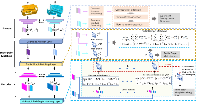
The structure of our framework is illustrated in Fig.1. We choose KPConv[16] as our feature backbone. Firstly, one point feature encoder consisting of three subsampling layers is used to downsample the given point cloud pairs to the sparse super points ($i.e.,$ $\hat{\mathbf{P}}\in\mathbb{R}^{N^{\prime}\times 3}$ and $\hat{\mathbf{Q}}\in\mathbb{R}^{M^{\prime}\times 3}$) and to extract associated features. Then we utilize the geometric attention layer (see section III-C) to give the super points embedding ($i.e.,$ $\mathbf{F}^{\hat{P}}\in\mathbb{R}^{{N^{\prime}}\times b}$ and $\mathbf{F}^{\hat{Q}}\in\mathbb{R}^{{M^{\prime}}\times b}$) and compute linear projected overlapping scores ($i.e.,$ $\mathbf{O}^{\hat{P}}$ and $\mathbf{O}^{\hat{Q}}$). After that, we deploy a partial graph matching optimization to enhance the super points’ ability to detect overlap regions (see section III-D). Next, we use a decoder that consists of three upsampling layers to decode the fine-level points, their corresponding features ($i.e.,$ $\mathbf{F}^{P}\in\mathbb{R}^{N\times 32}$ and $\mathbf{F}^{Q}\in\mathbb{R}^{N\times 32}$), and overlapping scores ($i.e.,$ $\mathbf{O}^{P}$ and $\mathbf{O}^{Q}$). Lastly, we take the mini-batch sampling to get several subsets from the overlap region and use full graph matching in each subset to refine the feature for global scaling matching (see section III-F).

Firstly, we downsample the raw point clouds to super points $\hat{\mathbf{P}}\in\mathbb{R}^{N^{\prime}\times 3}$ and $\hat{\mathbf{Q}}\in\mathbb{R}^{M^{\prime}\times 3}$ and generate associated features ${{\mathbf{F}}^{\hat{P}}}\in R^{N^{\prime}\times b}$ and ${{\mathbf{F}^{\hat{Q}}}\in R^{M^{\prime}\times b}}$. For super point embedding, we utilize the geometric attention layer[19, 26]. It encodes the local geometric structure embedding consisting of pair-wise distance (i.e., edge) and local triplet-wise angle in self-attention. It also uses cross-attention to do inter-point-cloud information exchange for overlap detection.

Local geometric structure embedding: For two points $p_{i}$ and $p_{j}$ in $\hat{\mathbf{P}}$, the point-wise distance is $\delta_{ij}=\lVert p_{i}-p_{j}\rVert_{2}$. To embed the angle, we select the k nearest neighbors $\mathbf{\kappa}_{i}$ for $p_{i}$. For each $\bar{p}_{x}\in\kappa_{i}$, the triplet-wise angle is computed as $\rho^{x}_{i,j}=\angle(\Delta_{x,i},\Delta_{j,i})$, where $\Delta_{j,i}:={\mathbf{p}_{j}}-{\mathbf{p}_{i}}$. We define geometric structure embedding as the combination of point-wise distance embedding and triplet-wise angle embedding:

$\displaystyle\mathbf{r}_{i,j}=\mathbf{r}_{i,j}^{D}\mathbf{W}^{D}+max_{x}(\mathbf{r}_{i,j,x}^{A}\mathbf{W}^{A}),$

(2)

where $\mathbf{r}_{i,j}^{D}$ and $\mathbf{r}_{i,j,x}^{A}$ are computed with a sinusoidal function on $\delta_{ij}/\sigma_{d}$ and $\rho^{x}_{i,j}/\sigma_{a}$. $\sigma_{d}$ and $\sigma_{a}$ are parameters to control the sensitivity to variations of distance and angle. $\mathbf{W}^{D},\mathbf{W}^{A}\in\mathbf{R}^{b\times b}$ are two linear projection layers. For points in $\hat{\mathbf{Q}}$, the embeddings are computed in the same way.

Self-attention and Cross-attention: Given the super points’ features and geometric structure embedding, we define the following geometric-aware self-attention:

	$\displaystyle a_{i,j}=softmax\left(\left[\frac{(\mathbf{x}_{i}\mathbf{W}^{q})(\mathbf{x}_{j}\mathbf{W}^{k}+\mathbf{r}_{i,j}\mathbf{W}^{g})^{\top}}{\sqrt{b}}\right]_{i,j}\right),$		(3)
	$\displaystyle\mathbf{z}_{i}=\sum_{j=1}^{\left|\hat{\mathbf{P}}\right|}a_{i,j}(\mathbf{x}_{j}\mathbf{W}^{v})$		(4)

where $W^{q},W^{k},W^{v},W^{g},\in\mathbf{R}_{b\times b}$ are linear projections of queries, keys, values, and geometric structure embeddings. Given the self-attention feature $Z^{\hat{\mathbf{P}}}$ and $Z^{\hat{\mathbf{Q}}}$, the cross-attention layer is define as:

	$\displaystyle a_{i,j}=softmax\left(\left[\frac{(\mathbf{z}_{i}^{\hat{\mathbf{P}}}\mathbf{W}^{q})(\mathbf{z}_{j}^{\hat{\mathbf{Q}}}\mathbf{W}^{k})^{\top}}{\sqrt{b}}\right]_{i,j}\right),$		(5)
	$\displaystyle\mathbf{z}_{i}^{\hat{\mathbf{P}}}=\sum_{j=1}^{\left|\hat{\mathbf{Q}}\right|}a_{i,j}(\mathbf{z}_{j}^{\hat{\mathbf{Q}}}\mathbf{W}^{v}).$		(6)

where $W^{q},W^{k},W^{v}\in\mathbf{R}_{b\times b}$ are linear projections of queries, keys, values.

By three interleaved attention layers of the configuration ’self/cross/self’, we get latent super point features $\mathbf{F}^{\hat{P}}\in R^{{N^{\prime}}\times b}$ and $\mathbf{F}^{\hat{Q}}\in R^{{M^{\prime}}\times b}$. To avoid symbol abuse, the initial input and final output features of the attention layers are all noted as $\mathbf{F}^{\hat{P}}\in R^{{N^{\prime}}\times b}$ and $\mathbf{F}^{\hat{Q}}\in R^{{M^{\prime}}\times b}$.

To enhance the super points’ abilities to capture isometry-preserving transformation properties, we deploy a Partial Graph Matching Optimizer (PGMO for short) to optimize the super point features. We utilize the super points ($i.e.,$ $\hat{\mathbf{P}}$ and $\hat{\mathbf{Q}}$) and their features ($i.e.,$ $\mathbf{F}^{\hat{P}}$ and $\mathbf{F}^{\hat{Q}}$) to compute the affinity matrices:

$$\small\begin{split}&{[\mathbf{C}^{\hat{P}}]}_{ij}=\lVert\mathbf{f}^{\hat{P}}_{i}-\mathbf{f}^{\hat{P}}_{j}\rVert_{2}+o^{\hat{p}_{i}}o^{\hat{p}_{j}}\alpha\lVert{\hat{\mathbf{p}}}_{i}-{\hat{\mathbf{p}}}_{j}\rVert_{2},\\ &{[\mathbf{C}^{\hat{Q}}]}_{ij}=\lVert\mathbf{f}^{\hat{Q}}_{i}-\mathbf{f}^{\hat{Q}}_{j}\rVert_{2}+o^{\hat{q}_{i}}o^{\hat{q}_{j}}\alpha\lVert{\hat{\mathbf{q}}}_{i}-{\hat{\mathbf{q}}}_{j}\rVert_{2},\\ &{[\mathbf{C}^{{\hat{P}\hat{Q}}}]}_{ij}=\lVert\mathbf{f}^{\hat{P}}_{i}-\mathbf{f}^{\hat{Q}}_{j}\rVert_{2},\end{split}$$

(7)

where $o^{\hat{p}_{i}}$ and $o^{\hat{q}_{j}}$ are overlapping scores of super points $\hat{\mathbf{p}}_{i}$ and $\hat{\mathbf{q}}_{j}$, and $\alpha$ is the hyper-parameter that controls the geometric similarity. Then we can solve the partial matching optimization to obtain the matching matrix:

$$\begin{split}&\min\limits_{\Gamma\in\Pi(\mathbf{p},\mathbf{q})}\sum_{i=1}^{N}\sum_{j=1}^{M}\mathbf{C}^{\hat{P}\hat{Q}}_{ij}\Gamma_{ij}+\frac{1}{2}\sum_{i,k=1}^{N}\sum_{j,l=1}^{M}\left({\mathbf{C}_{ik}^{\hat{P}}}-{\mathbf{C}_{jl}^{\hat{Q}}}\right)^{2}\Gamma_{ij}\Gamma_{kl}\\ &=\min\limits_{\Gamma\in\Pi(\mathbf{p},\mathbf{q})}\langle\mathbf{C}^{\hat{P}\hat{Q}},\Gamma\rangle+\langle\mathbf{L}(\mathbf{C}^{\hat{P}},\mathbf{C}^{\hat{Q}},\Gamma),\Gamma\rangle,\\ \end{split}$$

(8)

where $\langle.\rangle$ is inner product, $\mathbf{L}(\mathbf{C}^{\hat{P}},\mathbf{C}^{\hat{Q}},\Gamma)=\left[{\mathbf{L}_{jj^{\prime}}}\right]\in\mathbb{R}^{N{\times}M}$, each ${\mathbf{L}_{jj^{\prime}}}={\sum_{i,{i^{\prime}}}}\mathcal{L}\left(\mathbf{C}^{\hat{P}}_{ij},\mathbf{C}^{\hat{Q}}_{{i^{\prime}}{j^{\prime}}}\right){\Gamma_{ii^{\prime}}}$, and $\mathcal{L}(a,b)=\frac{1}{2}(a-b)^{2}$. The admissible couplings $\Pi(\mathbf{p},\mathbf{q})$ are defined as $\{\Gamma\in R_{+}^{N\times M}|\Gamma\mathbf{1}_{N}\leq\mathbf{1}_{M},\ \Gamma^{\top}\mathbf{1}_{M}\leq\mathbf{1}_{N},\mathbf{1}_{N}\Gamma\mathbf{1}_{M}=s\}$. The empirical distributions $(\mathbf{p},\mathbf{q})\in\Sigma_{N}\times\Sigma_{M}$, ${\Sigma_{N}}$ is a histogram of $N$ bins with $\left\{\mathbf{p}\in R^{N}_{+},\sum_{i}p_{i}=1\right\}$. We utilize the uniform distribution to initialize $(\mathbf{p},\mathbf{q})$. The partial transport mass $s$ is computed from the super points’ anchored patch[19] pairs whose overlap ratio is higher than 10$\%$.

Inspired by [27], by using mirror descent and Bregman projection ($i.e.,$ both the gradient and the projection are computed in the $KL$ metric) and setting the learning rate to $\frac{1}{\epsilon}$, we can transform problem (8) to a new $\epsilon$-convex entropic regularized optimal transport problem:

$$\Gamma^{n+1}=\arg\min\limits_{\Gamma\in\Pi(\mathbf{p},\mathbf{q})}\langle\bar{\mathbf{C}^{n}}-\epsilon log\Gamma^{n},\Gamma\rangle+\epsilon H(\Gamma),$$

(9)

where $\bar{\mathbf{C}^{n}}=L(\mathbf{C}^{\hat{P}},\mathbf{C}^{\hat{Q}},\Gamma^{n})+\mathbf{C}^{\hat{P}\hat{Q}}$ and the entropy $H(\Gamma)=-\sum_{i,j=1}^{N}\Gamma_{i,j}(log(\Gamma_{i,j})-1)$. According to Proposition 5 in [55], problem (9) is a partial transport problem with inequality constraints, which needs to use the Dykstra’s algorithm [56] to solve it. To accelerate the computing speed, motivated by the inexact proximal point algorithm (IPOT) in [30], the inner number of Dykstra’s iterations L is set to 1.

Given the super point features, we need to recover the original resolution point features. We leverage the NN upsampling and skip connections from the downsampling layers to form the decoder. We firstly concatenate the super point features $F^{\hat{P}}|F^{\hat{Q}}$, and the overlap scores ${O}^{\hat{P}}|{O}^{\hat{Q}}$, then go through upsampling decoder to get the fine-level ones: $F^{P}|F^{Q}$ and $O^{P}|O^{Q}$.

To enhance the fine-level points’ abilities to capture isometry-preserving transformation properties in the overlapping regions, we exploit a Full Graph Matching Optimizer Optimizer (FGMO for short) to optimize the point features:

$$\min\limits_{\Gamma\in{\hat{\Pi}(\mathbf{p},\mathbf{q})}}{\mathbf{J}}_{gm}({\Gamma})=\min\limits_{\Gamma}\lVert\mathbf{C}^{P}-\Gamma\mathbf{C}^{Q}\Gamma^{\top}\rVert_{F}+Tr(\mathbf{C}^{{PQ}^{\top}}\Gamma),\\$$

(10)

where $\mathbf{C}^{P}$ and $\mathbf{C}^{Q}$ are two affinity matrices of two graphs generated from points coordinates and features. $\mathbf{C}^{PQ}$ is the inter-graph affinity matrix or cost matrix. $\hat{\Pi}(\mathbf{p},\mathbf{q})$ is defined as $\{\Gamma\in R_{+}^{N\times M}|\Gamma\geq 0,\ \Gamma{\mathbf{1}_{N}}\leq{\mathbf{1}_{M}},\ \Gamma^{\top}{\mathbf{1}_{M}}\leq{\mathbf{1}_{N}}\}$. The definitions of $\mathbf{C}^{P}$, $\mathbf{C}^{Q}$, and $\mathbf{C}^{PQ}$ are as follows:

$$\begin{split}&{[\mathbf{C}^{P}]}_{ij}=\lVert\mathbf{f}^{P}_{i}-\mathbf{f}^{P}_{j}\rVert_{2}+\alpha\lVert\mathbf{p}_{i}-\mathbf{p}_{j}\rVert_{2},\\ &{[\mathbf{C}^{Q}]}_{ij}=\lVert\mathbf{f}^{Q}_{i}-\mathbf{f}^{Q}_{j}\rVert_{2}+\alpha\lVert\mathbf{q}_{i}-\mathbf{q}_{j}\rVert_{2},\\ &{[\mathbf{C}^{PQ}]}_{ij}=\lVert\mathbf{f}^{P}_{i}-\mathbf{f}^{Q}_{j}\rVert_{2},\end{split}$$

(11)

where $\alpha$ is a hyper-parameter that controls the geometric similarity.

Considering the large scale of fine level point cloud, we choose a reduced path following algorithm to efficiently solve the problem (10). Furthermore, we take the mini-batch method [54, 31] to accelerate solving the problem (10) in the overlap region:

We uniformly sample $K$ subsets from the fine-level overlap region, and each subset contains $m$ points. The average of $K$ mini-batch solutions would give an approximation of ground truth correspondences.

Coarse-level Overlap-aware Circle loss: Inspired by [19], the overlap ratio of patches anchored on the super points can weight the positive matching in loss to avoid the issue that the circle loss weights the positive samples equally. Given a pair of aligned coarse-level super points $\hat{\mathbf{P}}$ and $\hat{\mathbf{Q}}$. A pair of super points is positive if their anchor patch shares at least a 10% overlap ratio and negative if there is no overlap. All other pairs are dropped. For a super point $\hat{p}_{i}$, which at least has one positive patch in $\hat{\mathbf{Q}}$, we define the super points in $\hat{\mathbf{Q}}$ within radius $r_{\hat{p}}$ as $\mathbf{\xi}_{p}(\hat{p}_{i})$ and the super points outside a larger radius $r_{n}$ as $\mathbf{\xi}_{n}(\hat{p}_{i})$. Inspired by [18, 19], we sampled $n_{p}$ points from $\hat{P}_{\hat{p}}$, and the circle loss can be defined as follows:

$$\small{\mathscr{L}_{coc}^{\hat{\mathbf{P}}}}=\frac{1}{n_{p}}\sum_{i=1}^{n_{p}}log\left[1+\sum_{j\in\xi_{p}(\hat{p}_{i})}e^{\lambda_{i}^{j}\gamma(d_{i}^{j}-\Delta_{p})}+\sum_{k\in\xi_{n}(\hat{p}_{i})}e^{\gamma(\Delta_{n}-d_{i}^{k})}\right],$$

(13)

where $d_{i}^{j}=\lVert\mathbf{f}^{\hat{p}_{i}}-\mathbf{f}^{\hat{q}_{j}}\rVert_{2}$, $\gamma$ is a hyper-parameters and $\lambda_{i}^{j}$ is the overlap ratio of patches anchored on super point $\hat{\mathbf{p}}_{i}$ and $\hat{\mathbf{q}}_{j}$. Two empirical margins are defined as $\Delta_{p}:=0.1$ and $\Delta_{n}:=1.4$. The reverse loss $\mathscr{L}_{coc}^{\hat{\mathbf{Q}}}$ is also defined in the same way and the final circle loss is $\mathscr{L}_{coc}=\frac{1}{2}(\mathscr{L}_{coc}^{\hat{\mathbf{P}}}+\mathscr{L}_{coc}^{\hat{\mathbf{Q}}})$.

Coarse-level Partial Graph Matching loss: We calculate the intra-affinity and inter-affinity matrix for Eqn.(8) based on the coarse-level super points and features. The solution of the partial graph matching optimization (i.e., Eqn.(8)) can be treated as soft matching scores. The supervision on the matching score can be cast a binary classification, and we define a cross-entropy loss:

$\displaystyle\mathscr{L}_{cpgm}^{\hat{\mathbf{P}}}=\frac{1}{|\hat{\mathbf{P}}|}\sum_{i=1}^{\hat{\mathbf{P}}}\bar{m}^{\hat{p}_{i}}log(m^{\hat{p}_{i}})+(1-\bar{m}^{\hat{p}_{i}})log(1-m^{{\hat{p}}_{i}}),$

(14)

where ground truth $\bar{m}^{\bar{p}_{i}}$ is based on the overlap ratio of patch pairs that $\bar{m}^{\hat{p}_{i}}$ is 1 if the overlap ratio is greater than $10\%$, otherwise 0. The reverse loss $\mathscr{L}_{cpgm}^{\hat{\mathbf{Q}}}$ is also defined in the same way, and the final loss is $\mathscr{L}_{cpgm}=\frac{1}{2}(\mathscr{L}_{cpgm}^{\hat{\mathbf{P}}}+\mathscr{L}_{cpgm}^{\hat{\mathbf{Q}}})$.

Fine-Level mini-batch Graph Matching loss:

For every sample subset in the overlap region, the loss supervising the predicted matching scores is defined as:

$\displaystyle\mathscr{L}_{mbm}^{\mathbf{P}}=\frac{1}{|\mathbf{P}|}\sum_{i=1}^{\mathbf{P}}\bar{m}^{p_{i}}log(m^{p_{i}})+(1-\bar{m}^{p_{i}})log(1-m^{p_{i}}),$

(15)

where $\bar{m}^{p_{i}}$ is ground truth and $m^{p_{i}}$ is solution of Eqn.(10). The reverse loss $\mathscr{L}_{mbm}^{\mathbf{Q}}$ is also defined in the same way, and the final loss is $\mathscr{L}_{mbm}=\frac{1}{2}(\mathscr{L}_{mbm}^{\mathbf{P}}+\mathscr{L}_{mbm}^{\mathbf{Q}})$.

Fine-level overlap loss: To supervise the predicted overlap score on fine-level points, we use a binary classification loss for the overlap probability:

$\displaystyle\mathscr{L}_{o}^{\mathbf{P}}=\frac{1}{|\mathbf{P}|}\sum_{i=1}^{\mathbf{P}}\hat{o}^{p_{i}}log(o^{p_{i}})+(1-\hat{o}^{p_{i}})log(1-o^{{p}_{i}}),$

(16)

where ground truth label $\hat{o}^{p_{i}}$ is defined as

$\displaystyle\hat{o}^{p_{i}}=\begin{cases}1,\ \lVert\mathbf{T}(\mathbf{p}_{i})-{\mathbf{NN}}(\mathbf{T}(\mathbf{p}_{i}),\mathbf{Q})\rVert_{2}<\epsilon_{o}\\ 0,\ otherwise\end{cases},$

(17)

with overlap threshold $\epsilon_{o}$. The reverse loss $\mathscr{L}_{o}^{\mathbf{Q}}$ is computed in the same way and $\mathscr{L}_{o}=\frac{1}{2}(\mathscr{L}_{o}^{\mathbf{P}}+\mathscr{L}_{o}^{\mathbf{Q}})$. The final loss is defined as

$\displaystyle\mathscr{L}=\lambda_{c}(\mathscr{L}_{coc}+\mathscr{L}_{cpgm})+\lambda_{f}(L_{mbm}+\mathscr{L}_{o}),$

(18)

where $\lambda_{c}$ and $\lambda_{f}$ are the weights of the coarse-level and the fine-level losses, respectively. Following [18], we set $\lambda_{c}=\lambda_{f}=1$.

Following [17], we evaluate the proposed GMONet on indoor datasets 3DMatch[35] and 3DLoMatch [17] and outdoor KITTI odometry[57] benchmark.

Implementation and training: The proposed GMONet is implemented and tested with PyTorch [58] on Xeon(R) Gold 6230 and one NVIDIA RTX TITAN GPU. The network is trained 30 epochs on the 3DMatch/3DLoMatch dataset and 150 epochs on the KITTI odometry benchmark, all with Adam optimizer. The learning rates for 3DMatch/3DLoMatch and KITTI are set to 1e-4 and 5e-2, respectively. The batch size, weight decay, and momentum are set as 1, 1e-6, and 0.98, respectively. 3DMatch and KITTI’s matching radii are set to 5cm and 30cm, respectively. The hyper-parameter $\alpha$ in III-D is set to 0.01.

Dataset. 3DMatch[35] contains 62 scenes, divided into 46, 8, and 8 for training, validating, and testing, respectively. The overlap ratio of scanned pairs in 3DMatch is greater than $30\%$, while $10\%$-$30\%$ in 3DLoMatch.

Metrics. Following[35], we report performance with three metrics: (1) rigid Registration Recall (RR), the fraction of point cloud pairs whose correspondence RMSE below 0.2m. (2) Relative Rotation Error (RRE), the geodesic distance between estimated and ground truth rotation matrices. (3) Relative Translation Error (RTE), the Euclidean distance between the estimated and ground truth translation. RRE and RTE are calculated on the successfully matching scan pairs.

Interest point sampling. In the evaluation stage, we multiply the matching scores (normalized inner-product matrix from point features) and overlapping scores as the inlier confidence probabilities of points. Then a random sampling based on the confidence probability is applied to obtain the candidate point correspondences.

Results. We compare GMONet to recent feature-matching-based methods (FCGF[14], D3Feat[15], Predator[17], CoFiNet[18], GeoTransformer[19]). We adopt the same sampling strategy as GMONet to evaluate baseline GeoTransformer[19] for a fair comparison.

Tab.I shows that GMONet achieves the best registration recall to 92.1% on 3DMatch and 73.2% on 3DLoMatch with a sampling of 1000 points. Our method achieves relatively lower RTE and RRE on both 3DMatch and 3DLoMatch benchmarks. This reveals that, by adding two graph-matching optimizers in the learning stage, the point features indeed learn the isometry-preserving features and help select the ”rigid” candidate corresponding point more precisely.

Ablation studies. In the ablation studies, we take KPConv[16] as the backbone plus geometric attention layer, coarse-level overlap-aware circle loss, and fine-level overlap loss as the baseline. Then we add two levels of graph matching optimizer to conduct extensive experiments to ablate how these two constraints improve the feature representation. The default number of sampling points is set to 1000. Tab.II illustrates that by adding partial graph matching constraint on the coarse-level super points, the registration recall increases 0.58 percent points (pp) on 3DMatch and 0.6 pp on 3DLoMatch. The mini-batch graph matching constraint on fine-level points improves by 1.38 pp on 3DMatch and 3.0 pp on 3DLoMatch, respectively. These two constraints improve 2.08 pp and 5.0 pp on 3DMatch and 3DLoMatch, respectively.

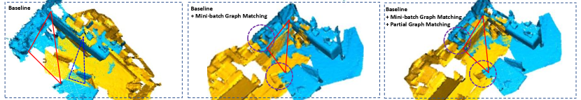
As visualized test case in Fig.2, without explicit isometric preserving constraints, based on the point features, RANSAC estimation would prefer such correspondences, $e.g.,$ edges near the vertexes of the deep blue triangle, that gives the max number of ”looks likely” correspondences (see the left column) in the overlap region. However, by explicitly adding two isometric preserving constraints, the point feature would recognize the critical correspondences ($e.g.,$ correspondences near the three vertexes of the red triangle in the middle column) even though the candidate corresponding points are far from each other in the euclidean space. Moreover, the graph matching optimization on coarse-level points further improves the registration’s precision (see points in the purple circle in middle and right columns). This illustrates that the two levels of graph matching optimizers help strengthen the points’ abilities to maintain isometry-preserving in feature space.

Computational Complexity. The running time of the two optimizers is listed in Tab.IV. Since we deploy two proposed optimizers only in the training stage and turn them off when inference, the run time is not a burden. The running time of the Partial Graph Matching Optimizer depends on the number of down-sampled super points, while Mini-batch Full Graph Matching Optimizer depends on the size of each sampled subset. Our default sampling number for each subset is set to 128.

Dataset. KITTI Odometry benchmark[57] consists of 11 sequences of point clouds scanned by LiDAR. We follow[17, 19] to use sequences 0-5 for training, 6-7 for validation, and 8-10 for testing.

Metrics. Following [17], we evaluate GMONet with three metrics: (1) rigid Registration Recall (RR), the fraction of successful registration pairs ($i.e.,$ RRE$<5^{\circ}$ and RTE$<$2m). The definitions of Relative Rotation Error (RRE) and Relative Translation Error (RTE) are the same as used in the 3DMatch benchmark.

Results. In the Tab.III, we compared GMONet with several state-of-the-art RANSAC-based methods: 3DFeat-Net[59], FCGF[14], D3Feat[15], Predator[17], CoFiNet[18], and GeoTransformer[19]. The quantitative results show that our method can handle outdoor scene registration and achieve competitive performance.

References

- [1] J. L. Schonberger and J.-M. Frahm, “Structure-from-motion revisited,” in Proceedings of the IEEE conference on computer vision and pattern recognition, 2016, pp. 4104–4113.
- [2] S. Choi, Q.-Y. Zhou, and V. Koltun, “Robust reconstruction of indoor scenes,” in Proceedings of the IEEE Conference on Computer Vision and Pattern Recognition, 2015, pp. 5556–5565.
- [3] J. Zhang and S. Singh, “Visual-lidar odometry and mapping: Low-drift, robust, and fast,” in 2015 IEEE International Conference on Robotics and Automation (ICRA). IEEE, 2015, pp. 2174–2181.
- [4] B. Drost, M. Ulrich, N. Navab, and S. Ilic, “Model globally, match locally: Efficient and robust 3d object recognition,” in 2010 IEEE computer society conference on computer vision and pattern recognition. Ieee, 2010, pp. 998–1005.
- [5] A. Zeng, K.-T. Yu, S. Song, D. Suo, E. Walker, A. Rodriguez, and J. Xiao, “Multi-view self-supervised deep learning for 6d pose estimation in the amazon picking challenge,” in 2017 IEEE international conference on robotics and automation (ICRA). IEEE, 2017, pp. 1386–1383.
- [6] H. Yang, J. Shi, and L. Carlone, “Teaser: Fast and certifiable point cloud registration,” IEEE Transactions on Robotics, vol. 37, no. 2, pp. 314–333, 2020.
- [7] Q. Li, S. Chen, C. Wang, X. Li, C. Wen, M. Cheng, and J. Li, “Lo-net: Deep real-time lidar odometry,” in Proceedings of the IEEE/CVF Conference on Computer Vision and Pattern Recognition, 2019, pp. 8473–8482.
- [8] J. Zhang and S. Singh, “Loam: Lidar odometry and mapping in real-time.” in Robotics: Science and Systems, vol. 2, no. 9. Berkeley, CA, 2014, pp. 1–9.
- [9] J. Lee, S. Kim, M. Cho, and J. Park, “Deep hough voting for robust global registration,” in Proceedings of the IEEE/CVF International Conference on Computer Vision, 2021, pp. 15 994–16 003.
- [10] X. Bai, Z. Luo, L. Zhou, H. Chen, L. Li, Z. Hu, H. Fu, and C.-L. Tai, “Pointdsc: Robust point cloud registration using deep spatial consistency,” in Proceedings of the IEEE/CVF Conference on Computer Vision and Pattern Recognition, 2021, pp. 15 859–15 869.
- [11] G. Mei, X. Huang, L. Yu, J. Zhang, and M. Bennamoun, “Cotreg: Coupled optimal transport based point cloud registration,” arXiv preprint arXiv:2112.14381, 2021.
- [12] Y. Shen, L. Hui, H. Jiang, J. Xie, and J. Yang, “Reliable inlier evaluation for unsupervised point cloud registration,” arXiv preprint arXiv:2202.11292, 2022.
- [13] H. Jiang, Y. Shen, J. Xie, J. Li, J. Qian, and J. Yang, “Sampling network guided cross-entropy method for unsupervised point cloud registration,” in Proceedings of the IEEE/CVF International Conference on Computer Vision, 2021, pp. 6128–6137.
- [14] C. Choy, J. Park, and V. Koltun, “Fully convolutional geometric features,” in Proceedings of the IEEE/CVF International Conference on Computer Vision, 2019, pp. 8958–8966.
- [15] X. Bai, Z. Luo, L. Zhou, H. Fu, L. Quan, and C.-L. Tai, “D3feat: Joint learning of dense detection and description of 3d local features,” in Proceedings of the IEEE/CVF conference on computer vision and pattern recognition, 2020, pp. 6359–6367.
- [16] H. Thomas, C. R. Qi, J.-E. Deschaud, B. Marcotegui, F. Goulette, and L. J. Guibas, “Kpconv: Flexible and deformable convolution for point clouds,” in Proceedings of the IEEE/CVF international conference on computer vision, 2019, pp. 6411–6420.
- [17] S. Huang, Z. Gojcic, M. Usvyatsov, A. Wieser, and K. Schindler, “Predator: Registration of 3d point clouds with low overlap,” in Proceedings of the IEEE/CVF Conference on computer vision and pattern recognition, 2021, pp. 4267–4276.
- [18] H. Yu, F. Li, M. Saleh, B. Busam, and S. Ilic, “Cofinet: Reliable coarse-to-fine correspondences for robust pointcloud registration,” Advances in Neural Information Processing Systems, vol. 34, pp. 23 872–23 884, 2021.
- [19] Z. Qin, H. Yu, C. Wang, Y. Guo, Y. Peng, and K. Xu, “Geometric transformer for fast and robust point cloud registration,” in Proceedings of the IEEE/CVF Conference on Computer Vision and Pattern Recognition, 2022, pp. 11 143–11 152.
- [20] Y. Li and T. Harada, “Lepard: Learning partial point cloud matching in rigid and deformable scenes,” in Proceedings of the IEEE/CVF Conference on Computer Vision and Pattern Recognition, 2022, pp. 5554–5564.
- [21] H. Wang, Y. Liu, Z. Dong, W. Wang, and B. Yang, “You only hypothesize once: Point cloud registration with rotation-equivariant descriptors,” arXiv preprint arXiv:2109.00182, 2021.
- [22] Z. J. Yew and G. H. Lee, “Regtr: End-to-end point cloud correspondences with transformers,” in Proceedings of the IEEE/CVF Conference on Computer Vision and Pattern Recognition, 2022, pp. 6677–6686.
- [23] A. Vaswani, N. Shazeer, N. Parmar, J. Uszkoreit, L. Jones, A. N. Gomez, Ł. Kaiser, and I. Polosukhin, “Attention is all you need,” Advances in neural information processing systems, vol. 30, 2017.
- [24] F. Zhou and F. De la Torre, “Factorized graph matching,” IEEE transactions on pattern analysis and machine intelligence, vol. 38, no. 9, pp. 1774–1789, 2015.
- [25] Q. Gao, F. Wang, N. Xue, J.-G. Yu, and G.-S. Xia, “Deep graph matching under quadratic constraint,” in Proceedings of the IEEE/CVF Conference on Computer Vision and Pattern Recognition, 2021, pp. 5069–5078.
- [26] Z. Chen, H. Chen, L. Gong, X. Yan, J. Wang, Y. Guo, J. Qin, and M. Wei, “Utopic: Uncertainty-aware overlap prediction network for partial point cloud registration,” arXiv preprint arXiv:2208.02712, 2022.
- [27] G. Peyré, M. Cuturi, and J. Solomon, “Gromov-wasserstein averaging of kernel and distance matrices,” in International Conference on Machine Learning. PMLR, 2016, pp. 2664–2672.
- [28] H. Xu, D. Luo, H. Zha, and L. C. Duke, “Gromov-wasserstein learning for graph matching and node embedding,” in International conference on machine learning. PMLR, 2019, pp. 6932–6941.
- [29] W. Liu, C. Zhang, J. Xie, Z. Shen, H. Qian, and N. Zheng, “Partial gromov-wasserstein learning for partial graph matching,” arXiv preprint arXiv:2012.01252, 2020.
- [30] Y. Xie, X. Wang, R. Wang, and H. Zha, “A fast proximal point method for computing exact wasserstein distance,” in Uncertainty in artificial intelligence. PMLR, 2020, pp. 433–453.
- [31] K. Nguyen, D. Nguyen, T. Pham, N. Ho et al., “Improving mini-batch optimal transport via partial transportation,” in International Conference on Machine Learning. PMLR, 2022, pp. 16 656–16 690.
- [32] P. J. Besl and N. D. McKay, “Method for registration of 3-d shapes,” in Sensor fusion IV: control paradigms and data structures, vol. 1611. Spie, 1992, pp. 586–606.
- [33] J. Yang, H. Li, and Y. Jia, “Go-icp: Solving 3d registration efficiently and globally optimally,” in Proceedings of the IEEE International Conference on Computer Vision, 2013, pp. 1457–1464.
- [34] Q.-Y. Zhou, J. Park, and V. Koltun, “Fast global registration,” in European conference on computer vision. Springer, 2016, pp. 766–782.
- [35] A. Zeng, S. Song, M. Nießner, M. Fisher, J. Xiao, and T. Funkhouser, “3dmatch: Learning local geometric descriptors from rgb-d reconstructions,” in Proceedings of the IEEE conference on computer vision and pattern recognition, 2017, pp. 1802–1811.
- [36] H. Deng, T. Birdal, and S. Ilic, “Ppfnet: Global context aware local features for robust 3d point matching,” in Proceedings of the IEEE conference on computer vision and pattern recognition, 2018, pp. 195–205.
- [37] H. Deng, T. Birdal, and S. Ilic, “Ppf-foldnet: Unsupervised learning of rotation invariant 3d local descriptors,” in Proceedings of the European Conference on Computer Vision (ECCV), 2018, pp. 602–618.
- [38] Y. Zhao, T. Birdal, H. Deng, and F. Tombari, “3d point capsule networks,” in Proceedings of the IEEE/CVF Conference on Computer Vision and Pattern Recognition, 2019, pp. 1009–1018.
- [39] M. Cuturi, “Sinkhorn distances: Lightspeed computation of optimal transport,” Advances in neural information processing systems, vol. 26, 2013.
- [40] K. Fu, S. Liu, X. Luo, and M. Wang, “Robust point cloud registration framework based on deep graph matching,” in Proceedings of the IEEE/CVF Conference on Computer Vision and Pattern Recognition, 2021, pp. 8893–8902.
- [41] H. W. Kuhn, “The hungarian method for the assignment problem,” Naval research logistics quarterly, vol. 2, no. 1-2, pp. 83–97, 1955.
- [42] R. Wang, J. Yan, and X. Yang, “Neural graph matching network: Learning lawler’s quadratic assignment problem with extension to hypergraph and multiple-graph matching,” IEEE Transactions on Pattern Analysis and Machine Intelligence, 2021.
- [43] R. Zass and A. Shashua, “Probabilistic graph and hypergraph matching,” in 2008 IEEE Conference on Computer Vision and Pattern Recognition. IEEE, 2008, pp. 1–8.
- [44] T. Vayer, L. Chapel, R. Flamary, R. Tavenard, and N. Courty, “Fused gromov-wasserstein distance for structured objects: theoretical foundations and mathematical properties,” arXiv preprint arXiv:1811.02834, 2018.
- [45] V. Titouan, N. Courty, R. Tavenard, and R. Flamary, “Optimal transport for structured data with application on graphs,” in International Conference on Machine Learning. PMLR, 2019, pp. 6275–6284.
- [46] E. Grave, A. Joulin, and Q. Berthet, “Unsupervised alignment of embeddings with wasserstein procrustes,” in The 22nd International Conference on Artificial Intelligence and Statistics. PMLR, 2019, pp. 1880–1890.
- [47] D. Alvarez-Melis, S. Jegelka, and T. S. Jaakkola, “Towards optimal transport with global invariances,” in The 22nd International Conference on Artificial Intelligence and Statistics. PMLR, 2019, pp. 1870–1879.
- [48] Z. Shen, J. Feydy, P. Liu, A. H. Curiale, R. San Jose Estepar, R. San Jose Estepar, and M. Niethammer, “Accurate point cloud registration with robust optimal transport,” Advances in Neural Information Processing Systems, vol. 34, pp. 5373–5389, 2021.
- [49] M. Eisenberger, A. Toker, L. Leal-Taixé, and D. Cremers, “Deep shells: Unsupervised shape correspondence with optimal transport,” Advances in Neural information processing systems, vol. 33, pp. 10 491–10 502, 2020.
- [50] M. Mandad, D. Cohen-Steiner, L. Kobbelt, P. Alliez, and M. Desbrun, “Variance-minimizing transport plans for inter-surface mapping,” ACM Transactions on Graphics (ToG), vol. 36, no. 4, pp. 1–14, 2017.
- [51] M. Frank and P. Wolfe, “An algorithm for quadratic programming,” Naval research logistics quarterly, vol. 3, no. 1-2, pp. 95–110, 1956.
- [52] M. Zaslavskiy, F. Bach, and J.-P. Vert, “A path following algorithm for the graph matching problem,” IEEE Transactions on Pattern Analysis and Machine Intelligence, vol. 31, no. 12, pp. 2227–2242, 2008.
- [53] K. Fatras, Y. Zine, R. Flamary, R. Gribonval, and N. Courty, “Learning with minibatch wasserstein: asymptotic and gradient properties,” arXiv preprint arXiv:1910.04091, 2019.
- [54] K. Fatras, T. Séjourné, R. Flamary, and N. Courty, “Unbalanced minibatch optimal transport; applications to domain adaptation,” in International Conference on Machine Learning. PMLR, 2021, pp. 3186–3197.
- [55] J.-D. Benamou, G. Carlier, M. Cuturi, L. Nenna, and G. Peyré, “Iterative bregman projections for regularized transportation problems,” SIAM Journal on Scientific Computing, vol. 37, no. 2, pp. A1111–A1138, 2015.
- [56] R. L. Dykstra, “An algorithm for restricted least squares regression,” Journal of the American Statistical Association, vol. 78, no. 384, pp. 837–842, 1983.
- [57] A. Geiger, P. Lenz, C. Stiller, and R. Urtasun, “Vision meets robotics: The kitti dataset,” The International Journal of Robotics Research, vol. 32, no. 11, pp. 1231–1237, 2013.
- [58] A. Paszke, S. Gross, F. Massa, A. Lerer, J. Bradbury, G. Chanan, T. Killeen, Z. Lin, N. Gimelshein, L. Antiga et al., “Pytorch: An imperative style, high-performance deep learning library,” Advances in neural information processing systems, vol. 32, 2019.
- [59] Z. J. Yew and G. H. Lee, “3dfeat-net: Weakly supervised local 3d features for point cloud registration,” in Proceedings of the European conference on computer vision (ECCV), 2018, pp. 607–623.