Graph and Temporal Convolutional Networks for 3D Multi-person
Pose Estimation in Monocular Videos
Abstract
Despite the recent progress, 3D multi-person pose estimation from monocular videos is still challenging due to the commonly encountered problem of missing information caused by occlusion, partially out-of-frame target persons, and inaccurate person detection. To tackle this problem, we propose a novel framework integrating graph convolutional networks (GCNs) and temporal convolutional networks (TCNs) to robustly estimate camera-centric multi-person 3D poses that does not require camera parameters. In particular, we introduce a human-joint GCN, which unlike the existing GCN, is based on a directed graph that employs the 2D pose estimator’s confidence scores to improve the pose estimation results. We also introduce a human-bone GCN, which models the bone connections and provides more information beyond human joints. The two GCNs work together to estimate the spatial frame-wise 3D poses, and can make use of both visible joint and bone information in the target frame to estimate the occluded or missing human-part information. To further refine the 3D pose estimation, we use our temporal convolutional networks (TCNs) to enforce the temporal and human-dynamics constraints. We use a joint-TCN to estimate person-centric 3D poses across frames, and propose a velocity-TCN to estimate the speed of 3D joints to ensure the consistency of the 3D pose estimation in consecutive frames. Finally, to estimate the 3D human poses for multiple persons, we propose a root-TCN that estimates camera-centric 3D poses without requiring camera parameters. Quantitative and qualitative evaluations demonstrate the effectiveness of the proposed method. Our code and models are available at https://github.com/3dpose/GnTCN.
Introduction
Significant progress has been made in 3D human pose estimation in recent years, e.g. (Sun et al. 2019a; Pavllo et al. 2019; Cheng et al. 2019, 2020). In general, existing methods can be classified as either top-down or bottom-up. Top-down approaches use human detection to obtain the bounding box of each person, and then perform pose estimation for every person. Bottom-up approaches are human-detection free and can estimate the poses of all persons simultaneously. Top-down approaches generally demonstrate more superior performance in pose estimation accuracy, and are suitable for many applications that require high pose estimation precision (Pavllo et al. 2019; Cheng et al. 2020); while bottom-up approaches are better in efficiency (Cao et al. 2017, 2019). In this paper, we aim to further improve 3D pose estimation accuracy, and thus push forward the frontier of the top-down approaches.

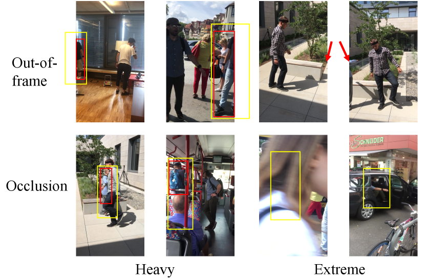
Most top-down methods focus on single person and define a 3D pose in a person-centric coordinate system (e.g., pelvis-based origin), which cannot be extended to multiple persons. Since for multiple persons, all the estimated skeletons need to reside in a single common 3D space in correct locations. The major problem here is that by applying the person-centric coordinate system, we lose the location of each person in the scene, and thus we do not know where to put them, as shown in Fig. 1, second row. Another major problem of multiple persons is the missing information of the target persons, due to occlusion, partially out-of-frame, inaccurate person detection, etc. For instance, inter-person occlusion may confuse human detection (Lin and Lee 2020; Sárándi et al. 2020), causing erroneous pose estimation (Li et al. 2019; Umer et al. 2020), and thus affect the 3D pose estimation accuracy (as shown in Fig. 1, third row). Addressing these problems is critical for multi-person 3D pose estimation from monocular videos.
In this paper, we exploit the use of the visible human joints and bone information spatially and temporally utilizing GCNs (Graph Convolutional Networks) and TCNs (Temporal Convolutional Networks). Unlike most existing GCNs, which are based on undirected graphs and only consider the connection of joints, we introduce a directed graph that can capture the information of both joints and bones, so that the more reliably estimated joints/bones can influence the unreliable ones caused by occlusions (instead of treating them equally as in undirected graphs). Our human-joint GCN (in short, joint-GCN) employs the 2D pose estimator’s heatmap confidence scores as the weights to construct the graph’s edges, allowing the high-confidence joints to correct low-confidence joints in our 3D pose estimation. While our human-bone GCN (in short, bone-GCN) makes use of the confidence scores of the part affinity field (Cao et al. 2019) to provide complementary information to the joint GCN. The features produced by the joint- and bone-GCNs are concatenated and fed into our fully connected layers to estimate a person-centric 3D human pose.
Our GCNs focus on recovering the spatial information of target persons in a frame-by-frame basis. To increase the accuracy across the input video, we need to put more constraints temporally, both in terms of the smoothness of the motions and the correctness of the whole body dynamics (i.e., human dynamics). To achieve this, we first employ a joint-TCN that takes a sequence of the 3D poses produced by the GCN module as input, and estimate the person-centric 3D pose of the central frame. The joint-TCN imposes a smoothness constraint in its prediction and also imposes the constraints of human dynamics. However, the joint-TCN can estimate only person-centric 3D poses (not camera-centric). Also, the joint-TCN is not robust to occlusion. To resolve the problems, we introduce two new types of TCNs: root-TCN and velocity-TCN.
Relying on the output of the joint-TCN, our root-TCN produces the camera-centric 3D poses, where the coordinates of the person center, i.e. the pelvis, are in the camera coordinate system. The root-TCN is based on the weak perspective camera model, and does not need to be trained with large variation of camera parameters, since it estimates only the relative depth, . Our velocity-TCN takes the person-centric 3D poses and the velocity from previous frames as input, and estimates the velocity at the current frame. Our velocity-TCN estimates the current pose based on the previous frames using motion cues. Hence, it is more robust to missing information, such as in the case of occlusion. The reason is because the joint-TCN focuses on the correlations between past and future frames regardless of the trajectory, while the velocity-TCN focuses on the motion prediction, and thus makes the estimation more robust.
In summary, our contributions are listed as follows.
-
•
Novel directed graph-based joint- and bone-GCNs to estimate 3D poses that can predict human 3D poses even though the information of the target person is incomplete due to occlusion, partially out-of-frame, inaccurate human detection, etc.
-
•
Root-TCN that can estimate the camera-centric 3D poses using the weak perspective projection without requiring camera parameters.
-
•
Combination of velocity- and joint-TCNs that utilize velocity and human dynamics for robust 3D pose estimation.
Related Works
3D human pose estimation in video
Recent 3D human pose estimation methods utilize temporal information via recurrent neural network (RNN) (Hossain and Little 2018; Lee, Lee, and Lee 2018; Chiu et al. 2019) or TCN (Pavllo et al. 2019; Cheng et al. 2019; Sun et al. 2019b; Cheng et al. 2020) improve the temporal consistency and show promising results on single-person video datasets such as HumanEva-I, Human3.6M, and MPI-INF-3DHP (Sigal, Balan, and Black 2010; Ionescu et al. 2014; Mehta et al. 2017a), but they still suffer from the inter-person occlusion issue when applying to multi-person videos. Although a few works take occlusion into account (Ghiasi et al. 2014; Charles et al. 2016; Belagiannis and Zisserman 2017; Cheng et al. 2019, 2020), in a top-down framework, it is difficult to reliably estimation 3D multi-person human poses in videos due to erroneous detection and occlusions. Moreover, none of these method estimate camera-centric 3D human poses.
Monocular 3D human pose estimation
Earlier approaches that tackle camera-centric 3D human pose from monocular camera require camera parameters as input or assume fixed camera pose to project the 2D posture into camera-centric coordinate (Mehta et al. 2017b, 2019; Pavllo et al. 2019). As a result, these methods are inapplicable for wild videos where camera parameters are not available. Removing the requirement of camera parameters has drawn researcher’s attention recently. Moon et al. (Moon, Chang, and Lee 2019) first propose to learn a correction factor for a person’s root depth estimation from a single image. Several recent works (Li et al. 2020; Lin and Lee 2020; Zhen et al. 2020) show improved performance compared with (Moon, Chang, and Lee 2019). Li et al. (Li et al. 2020) develop an integrated method for detection, person-centric pose, and depth estimation from a single image. Lin et al. (Lin and Lee 2020) propose to formulate the depth regression as a bin index estimation problem. Zhen et al. (Zhen et al. 2020) propose to estimate 2.5D representation of body parts first and then reconstruct 3D human pose. Unlike their approach, our method is video-based where temporal information is utilized by TCN on top of GCN output, which leads to improved 3D pose estimation.

GCN for pose estimation
Graph convolutional network (GCN) has been applied to 2D or 3D human pose estimation in recent years (Zhao et al. 2019; Cai et al. 2019; Ci et al. 2019; Qiu et al. 2020). Zhao et al. (Zhao et al. 2019) propose a graph neural network architecture to capture local and global node relationship and apply the proposed GCN for single-person 3D pose estimation from image. Ci et al (Ci et al. 2019) explore different network structures by comparing fully connected network and GCN and develop a locally connected network to improve the representation capability for single-person 3D human pose estimation from image as well. Cai et al. (Cai et al. 2019) construct an undirected graph to model the spatial-temporal dependencies between different joints for single-person 3D pose estimation from video data. Qiu et al. (Qiu et al. 2020) develop a dynamic GCN framework for multi-person 2D pose estimation from a image. Our method is different from all these methods in terms of we propose to use directed graph to incorporate heatmap and part affinity field confidence in graph construction, which brings the benefit of overcoming the limitation of human detection on top-down pose estimation methods.
Method
The overview of our framework is shown as Fig. 2. Having obtained the 2D poses from the 2D pose estimator, the poses are normalized so that they are centered at the root point, which is at the hip of human body. Each pose is then fed into our joint- and bone-GCNs to obtain its 3D full pose, despite the input 2D pose might be incomplete. Finally, a 3D full pose sequence is fed into the joint-TCN, root-TCN, and velocity-TCN to obtain the camera-centric 3D human poses that have smooth motion and comply with natural human dynamics.
Joint-GCN and Bone GCN
Existing top-down methods are erroneous when the target human bounding box is incorrect, due to missing information (occlusion, partially out-of-frame, blur, etc.). To address this common problem, we introduce joint-GCN and bone-GCN that can correct the 3D poses from inaccurate 2D pose estimator. These GCNs work on a frame-by-frame basis.
Following the structure of the human body, we assign the coordinates of the human joints from the 2D pose estimator to each vertex of our graph, and establish connections between each pair of the joints. Unlike most GCNs, which are based on an undirected graph, we propose a GCN based on a directed graph. The directed graph allows us to propagate information more from high-confident joints to low-confident ones, and thus reduces the risk of propagating erroneous information (e.g., occluded joints or missing joints) in the graph. In other words, the low-confident joints contribute less to the message propagation than the high-confident ones. Details of the directed graph are available in the supplementary material.
The joint-GCN uses the 2D joints as the vertices and the confidence scores of the 2D joints as the edge weights, while the bone-GCN uses the confidence scores of part affinity field (Cao et al. 2017)) as the edge weights. The features produced by the two GCNs are concatenated together and fed to a Multi Layer Perceptron to obtain the person-centric 3D pose estimation.
In GCNs, the message is propagated according to adjacent matrix, which indicates the edge between each pair of vertices. The adjacency matrix is formed by the following rule:
| (1) |
where is the heatmap from the 2D pose estimator. stands for the number of the order of neighboring vertices, which means the number of hops required to reach vertex from vertex . This formation of adjacency imposes more weight for close vertices and less for distance vertices.
The forward propagation of each GCN layer can be expressed as:
| (2) |
where is the feature transformation function, and is the learnable parameter of layer . To learn a network with strong generalization ability, we follow the idea of Graph SAGE (Hamilton, Ying, and Leskovec 2017) to learn a generalizable aggregator, which is formulated as:
| (3) |
where is the output of layer in the GCN and stands for the concatenation operation. is the normalized adjacency matrix. Since our method is based on a directed graph, which uses a non-symmetric adjacency matrix, the normalization is instead of in (Kipf and Welling 2016), and are the indegree of vertices and , respectively. This normalization ensures that the indegree of each vertex sums to , which prevents numerical instability.
Our joint-GCN considers only human-joints and does not include the information of bones, which can be critical for the cases when the joints are missing due to occlusion or other reasons. To exploit the bone information, we created a bone-GCN. First, we construct the incidence matrix of shape to represent the bone connections, where each row represents an edge and the columns represent vertices. For each bone, the parent joint is assigned with and the child joint is assigned with . Second, the incidence matrix is multiplied with the joint matrix to obtain the bone matrix , which will be further fed into our bone-GCN.
In joint matrix , each row stands for the 2D coordinate of a joint. Unlike our joint-GCN, where the adjacency matrix is drawn from the joint heatmap produced by 2D pose estimator, our human-bone GCN utilizes the confidence scores from the part affinity field, following the method of (Cao et al. 2017), as the adjacency. Finally, the outputs from our human-joint GCN and human-bone GCN are concatenated together and fed into an MLP (Multi-layer Perceptron). The loss function we use is the loss between GCN 3D joints output and 3D ground-truth skeleton , which is
In the training stage, to obtain sufficient variation and to increase the robustness of our GCNs, we use not only the results from our 2D pose estimator, but also augmented data from our ground-truths. Each joint is assigned with a random confidence score and random noise.
Root-TCN
In most of the videos, the projection can be modelled as weak perspective:
| (4) |
where and are the image coordinates, and are the camera coordinates. stands for the focal length and camera centers, respectively. Thus we have:
| (5) |
By assuming as the image center, which is applicable for most cameras, the only parameters we need to estimate is depth and focal length . To be more practical, we jointly estimate , instead of estimating them separately. This enables our method to be able to take wild videos that the camera parameters are unknown.
According to the weak perspective assumption, the scale of a person in a frame indicates the depth in the camera coordinates. Hence, we propose a network, root Temporal Convolutional Network (root-TCN), to estimate the from 2D pose sequences. We first normalize each 2D pose by scaling the average joint-to-pelvis distance to , using a scale factor . Then we concatenate the normalized pose , scale factor , as well as the person’s center in the frame as , and feed a list of such concatenated features in a local temporal window into the TCN for depth estimation in the camera coordinates.
As directly learning is not easy to converge, we transform this regression problem into a classification problem. For each video, we divide the depth into discrete ranges, set to 60 in our experiments, and our root-TCN outputs a vector with length as , where indicates the probability that is within the th discrete range. Then, we apply Soft-argmax to this vector to get the final continuous estimation of the depth as:
| (6) |
where is the time stamp, and is half of the temporal window’s size. This improves the training stability and reduces the risk of large errors.
The loss function for the depth estimation is defined as the mean squared error between the ground truth and predictions, expressed as , where is the predicted value, and denotes the ground truth. According to Eq.(5), we can calculate the coordinates for the person’s center as .
Joint-TCN and Velocity-TCN
To increase the accuracy of the 3D poses across the input video, we impose temporal constraints, by employing a temporal convolutional network (TCN) (Cheng et al. 2020) that takes a sequence of consecutive 3D poses as input. We call this TCN a joint-TCN, which is trained using various 3D poses and their augmentation, and hence capture human dynamics. The joint-TCN outputs the person-centric 3D pose, . The TCN utilizes temporal information to interpolate the poses of occluded frames with temporal information.
However, when persons get close and occlude each other, there may be fewer visible joints belonging to a person and more distracting joints from other persons. To resolve the problem, in addition to the joint-TCN, we propose a velocity-based estimation network, velocity-TCN, which takes the 3D joints and their velocities as input, and predicts the velocity of all joints as:
| (7) |
where stands for the 2D pose and denotes the velocity at time . TCNv is the velocity-TCN. The velocity here is proportional to according to Eq. (5). We normalize the velocity both in training and testing. With estimated , we can obtain the coordinate , where and are estimated coordinates at time and . The calculation of is discussed later in Eq.(8).
The joint-TCN predicts the joints by interpolating the past and future poses, while our velocity-TCN predicts the future poses using motion cues. Both of them are able to handle the occlusion frames, but the joint-TCN focuses on the connection between past and future frames regardless of the trajectory, while the velocity-TCN focuses on the motion prediction, which can handle a motion drift. To leverage the benefits of both, we introduce an adaptive weighted average of their estimated coordinates and .
We utilize the 2D pose tracker (Umer et al. 2020) to detect and track human poses in the video. In the tracking procedure, we regard the heatmaps with less than confidence value as occluded joints, and the pose with less than non-occluded joints as the occluded pose. By doing this, we obtain the occlusion information for both joints and frames. Note that the values here are obtained empirically through our experiments. Suppose we find an occlusion duration from to for a person, then we generate the final coordinates as:
| (8) |
where . For frames that are closer to occlusion duration boundaries, we trust more; for those are far from occlusion boundaries, we trust more. The velocity-TCN loss is the loss between the predicted 3D points at and ground-truth 3D points.
Experiments
MuPoTS-3D is a 3D multi-person testing set with both indoor and outdoor scenes (Mehta et al. 2018). The ground-truth 3D pose of each person in the video is obtained from multi-view markerless capture, which is suitable for evaluating 3D multi-person pose estimation performance in both person-centric and camera-centric coordinates. Unlike previous methods (Moon, Chang, and Lee 2019) using the training set (MuCo-3DHP) to train their models and then do evaluation on MuPoTS-3D, we use MuPoTS-3D for testing only without fine-tuning.
3DPW is an outdoor multi-person dataset for 3D human pose reconstruction (von Marcard et al. 2018). Following previous methods (Kanazawa et al. 2019; Sun et al. 2019b), we use 3DPW for testing only without any fine-tuning. The ground-truth of 3DPW is SMPL 3D mesh model (Loper et al. 2015), where the definition of joints differs from the one commonly used in 3D human pose estimation (skeleton-based) like Human3.6M (Tripathi et al. 2020), so it is unfair to evaluate skeleton-based methods on it even after joint adaption or scaling. To perform a fair comparison, we select an occlusion subset from the 3DPW test set (please refer to the supplementary material for details). And the performance change of a method between the full test set and the subset indicates how well the method can handle the missing information problem caused by occlusions.
Human3.6M is a widely used dataset and benchmark for 3D human pose estimation (Ionescu et al. 2014). It contains 3.6 million single-person indoor images captured by the MoCap system, which is suitable for evaluation of single-person pose estimation and camera-centric coordinates prediction. Following previous works (Hossain and Little 2018; Pavllo et al. 2019; Wandt and Rosenhahn 2019), the subject 1,5,6,7,8 are used for training, and 9 and 11 for testing.
Evaluation and Implementation MPJPE, PA-MPJPE, PCK, and are used for person-centric pose estimation evaluation. and PCKabs are used for camera-centric pose estimation evaluation. Each GCN and TCN is trained for 100 epochs with initial learning rate , more details are available in the supplementary material.
| Method | PCK | PCKabs | ||
|---|---|---|---|---|
| Baseline | 24.1 | 32.9 | 74.4 | 29.8 |
| Baseline (GT box) | 28.5 | 34.2 | 78.9 | 31.2 |
| Baseline + GCNs | 35.4 | 39.7 | 83.2 | 35.1 |
| Baseline + TCNs | 38.4 | 43.1 | 85.3 | 38.7 |
| Full model | 45.2 | 48.9 | 87.5 | 45.7 |
Ablation Studies In Table 1, we provide the results of an ablation study to validate the major components of the proposed framework. MuPoTS-3D is used as it has been used for 3D multi-person pose evaluation in person-centric and camera-centric coordinates (Moon, Chang, and Lee 2019). and PCK metrics are used to evaluate person-centric 3D pose estimation performance, and PCKabs metrics are used to evaluate camera-centric 3D pose (i.e., camera-centric coordinate) estimation following (Moon, Chang, and Lee 2019).
| Method | PCK | PCKabs | ||
| Joint* GCN | 24.1 | 27.3 | 73.1 | 25.6 |
| Joint GCN | 28.5 | 30.1 | 76.8 | 29.0 |
| Joint + Bone* GCN | 28.4 | 31.9 | 78.1 | 29.7 |
| Joint + Bone GCN | 33.4 | 37.9 | 82.6 | 34.3 |
| Joint + Bone + Aug. | 35.4 | 39.7 | 83.2 | 35.1 |
| Joint TCN | 43.1 | 45.8 | 86.2 | 42.6 |
| Joint + Velocity | 45.2 | 48.9 | 87.5 | 45.7 |
In particular, we use the joint-TCN with time window 1 plus a root-TCN with time window 1 as a baseline for both person-centric and camera-centric coordinate estimation as shown at the 1st row in Table 1. We use the baseline with ground-truth bounding box (i.e., perfect 2D tracking) as a second baseline to illustrate even with perfect detection bounding box the baseline still performs poorly because it cannot deal with occlusion and distracting joints from other persons. On the contrary, we can see significant performance (e.g., improvement against the baseline in PCKabs) improvements after adding the proposed GCN and TCN modules as shown in row 3 - 5 in Table 1. The benefits from the TCNs are slightly larger than those from the joint and bone GCNs as temporal information is used by the TCNs while GCNs only use frame-wise information. Lastly, our full model shows the best performance, with improvement against the baseline in terms of PCKabs.
We perform a second ablation study to break down the different pieces in our GCN and TCN modules to show the effectiveness of each individual component in Table 2. We observe the undirected graph-based GCN performs the worst as shown in the 1st row. Our joint-GCN, bone-GCN, and data augmentation (applying random cropping and scaling) show improved performance in row 2 - 4. On top of the full GCN module, we also show the contribution of the joint-TCN and velocity-TCN in row 5 - 6 (row 6 is our full model). Similar to Table 1 we can see the TCN module brings more improvement compared with the GCN module as temporal information is used.
| Group | Method | PCK | PCKabs |
|---|---|---|---|
| Mehta et al. (2018) | 65.0 | n/a | |
| Person- | Rogez et al., (2019) | 70.6 | n/a |
| centric | Cheng et al. (2019) | 74.6 | n/a |
| Cheng et al. (2020) | 80.5 | n/a | |
| Moon et al. (2019) | 82.5 | 31.8 | |
| Camera- | Lin et al. (2020) | 83.7 | 35.2 |
| centric | Zhen et al. (2020) | 80.5 | 38.7 |
| Li et al. (2020) | 82.0 | 43.8 | |
| Our method | 87.5 | 45.7 |
Quantitative Results To compare with the state-of-the-art (SOTA) methods in 3D multi-person human pose estimation, we perform evaluations on MuPoTS-3D as shown in Table 3. Please note our network is trained only on Human3.6M to have a fair comparison with other methods (Cheng et al. 2019, 2020). As the definition of keypoints in MuPoTS-3D is different from the one where our model is trained on, we use joint adaptation (Tripathi et al. 2020) to transfer the definition of keypoints. Among the methods in Table 3, (Moon, Chang, and Lee 2019; Lin and Lee 2020; Li et al. 2020) are fine-tuned on 3D training set MuCo-3DHP.
Regarding to the performance on MuPoTS-3D, our camera-centric pose estimation accuracy beat the SOTA (Li et al. 2020) by on PCKabs. A few papers reported their results on , where (Moon, Chang, and Lee 2019) is 31.0, (Lin and Lee 2020) is 39.4, and our result is 45.2, where we beat the SOTA (Lin and Lee 2020) by . We also compare with other methods on person-centric 3D pose estimation, and get improvement of on PCK against the SOTA (Lin and Lee 2020). Please note we do not fine-tune on MuCo-3DHP like others (Moon, Chang, and Lee 2019; Lin and Lee 2020; Li et al. 2020), which is the training dataset for evaluation on MuPoTS-3D. Moreover, the SOTA method (Lin and Lee 2020) on person-centric metric PCK shows poor performance on PCKabs (ours vs theirs: 45.7 - 35.2, improvement), and the SOTA method (Li et al. 2020) on camera-centric metric PCKabs has mediocre performance on PCK (ours vs theirs: 87.5 vs 82.0, improvement). All of these results clearly show that our method not only surpasses all existing methods, but also is the only method that is well-balanced in both person-centric and camera-centric 3D multi-person pose estimation.
| Dataset | Method | PA-MPJPE | |
|---|---|---|---|
| Dabral et al. (2018) | 92.2 | n/a | |
| Doersch et al. (2019) | 74.7 | n/a | |
| Kanazawa et al. (2019) | 72.6 | n/a | |
| Cheng et al. (2020) | 71.8 | n/a | |
| Original | Sun et al. (2019b) | 69.5 | n/a |
| Kolotouros et al. (2019)* | 59.2 | n/a | |
| Kocabas et al., (2020)* | 51.9 | n/a | |
| Our method | 64.2 | n/a | |
| Cheng et al. (2020) | 96.1 | +24.1 | |
| Sun et al. (2019b) | 94.1 | +24.6 | |
| Subset | Kolotouros et al. (2019)* | 88.9 | +29.7 |
| Kocabas et al., (2020)* | 82.5 | +30.6 | |
| Our method | 85.7 | +21.5 |
3DPW dataset (von Marcard et al. 2018) is a new 3D multi-person human pose dataset that contains multi-person outdoor scenes for person-centric pose estimation evaluation. Following previous works (Kanazawa et al. 2019; Sun et al. 2019b), 3DPW is only used for testing and the PA-MPJPE values on test set are shown in Table 4. As discussed in the Datasets section, the ground-truth definitions are different between 3D pose reconstruction and estimation where the ground-truth of 3DPW is SMPL mesh model, even we follow (Tripathi et al. 2020) to perform joint adaptation to transform the estimated joints but still have a disadvantage, and the PA-MPJPE values cannot objectively reflect the performance of skeleton-based pose estimation methods.
As aforementioned, we select a subset out of the original test set with the largest detection errors, and run the code of the top-performing methods in Table 4 on this subset for comparison. Table 4 shows that even with the disadvantage of different definition of joints, our method is the 3rd best on the original testing test, and becomes the 2nd best on the subset where the difference to the best one (Kocabas, Athanasiou, and Black 2020) is greatly shrunk. More importantly, the of PA-MPJPE between the original testing set and the subset in the 4th column in Table 4, our method shows the least error increase compared with all other top-performing methods. In the particular, the two best methods (Kolotouros et al. 2019; Kocabas, Athanasiou, and Black 2020) on the original testing set show 29.7 and 30.6 mm error increase while our method shows only 21.5 mm. The performance change of PA-MPJPE between the original testing set and the subset clearly demonstrates that our method is the best in terms of solving the missing information problem which is critical for 3D multi-person pose estimation.
| Group | Method | MPJPE | PA-MPJPE |
|---|---|---|---|
| Hossain et al., (2018) | 51.9 | 42.0 | |
| Wandt et al., (2019)* | 50.9 | 38.2 | |
| Person- | Pavllo et al., (2019) | 46.8 | 36.5 |
| centric | Cheng et al., (2019) | 42.9 | 32.8 |
| Kocabas et al., (2020) | 65.6 | 41.4 | |
| Kolotouros et al. (2019) | 41.1 | n/a | |
| Moon et al., (2019) | 54.4 | 35.2 | |
| Camera- | Zhen et al., (2020) | 54.1 | n/a |
| centric | Li et al., (2020) | 48.6 | 30.5 |
| Ours | 40.9 | 30.4 |

In order to further illustrate the effectiveness of both person-centric and camera-centric 3D pose estimation of our method, we perform evaluations on the widely used single-person dataset, Human3.6M. To evaluate camera-centric pose estimation, we use mean root position error (MPRE), a new evaluation metric proposed by (Moon, Chang, and Lee 2019). Our result is 88.1 mm, the result of (Moon, Chang, and Lee 2019) is 120 mm, the result of (Lin and Lee 2020) is 77.6 mm. Our method outperforms the result of (Moon, Chang, and Lee 2019) by a large margin: 31.9 mm error reduction and 26% improvement. Although depth estimation focused method (Lin and Lee 2020) shows better camera-centric performance on this single-person dataset Human3.6M, their camera-centric result on multi-person dataset MuPoTS-3D is much worse than ours (ours vs. theirs in PCKabs: 45.7 - 35.2, improvement). Camera-centric 3D human pose estimation is for multi-person pose estimation, good performance only on single-person dataset is not enough to solve the problem.
To compare with most of the existing methods that evaluate person-centric 3D pose estimation on Human3.6M using MPJPE and PA-MPJPE, we report our results using the same metrics in Table 5. As Human3.6M contains only single-person videos, we do not expect to our method bring much improvement. It is observed that our method is comparable with the SOTA methods. In addition, although our method shows improved performance over others that use kinematic constraints (Wandt and Rosenhahn 2019; Cheng et al. 2019) because of our GCNs and TCNs, adding kinematic constraints could potentially improve our performance further (Akhter and Black 2015; Kundu et al. 2020).
Qualitative Results As shown in Figure 3, our full model can better handle occlusions and incorrect detection compared with the baselines and the relative positions among all persons are well captured without camera parameters. More comparisons against SOTA methods and qualitative results on wild videos are available in the supplementary material.
Conclusion
We propose a new framework to unify GCNs and TCNs for camera-centric 3D multi-person pose estimation. The proposed method successfully handles missing information due to occlusion, out-of-frame, inaccurate detections, etc., in videos and produces continuous pose sequences. Experiments on different datasets validate the effectiveness of our framework as well as our individual modules.
Acknowledgements
This research/project is supported by the National Research Foundation, Singapore under its Strategic Capability Research Centres Funding Initiative. Any opinions, findings and conclusions or recommendations expressed in this material are those of the author(s) and do not reflect the views of National Research Foundation, Singapore.
References
- Akhter and Black (2015) Akhter, I.; and Black, M. J. 2015. Pose-conditioned joint angle limits for 3D human pose reconstruction. In Proceedings of the IEEE conference on computer vision and pattern recognition, 1446–1455.
- Arnab, Doersch, and Zisserman (2019) Arnab, A.; Doersch, C.; and Zisserman, A. 2019. Exploiting temporal context for 3D human pose estimation in the wild. In Proceedings of the IEEE Conference on Computer Vision and Pattern Recognition, 3395–3404.
- Belagiannis and Zisserman (2017) Belagiannis, V.; and Zisserman, A. 2017. Recurrent Human Pose Estimation. In International Conference on Automatic Face and Gesture Recognition (FG). IEEE.
- Cai et al. (2019) Cai, Y.; Ge, L.; Liu, J.; Cai, J.; Cham, T.-J.; Yuan, J.; and Thalmann, N. M. 2019. Exploiting spatial-temporal relationships for 3d pose estimation via graph convolutional networks. In Proceedings of the IEEE International Conference on Computer Vision, 2272–2281.
- Cao et al. (2019) Cao, Z.; Hidalgo, G.; Simon, T.; Wei, S.-E.; and Sheikh, Y. 2019. OpenPose: Realtime Multi-Person 2D Pose Estimation using Part Affinity Fields. IEEE Transactions on Pattern Analysis and Machine Intelligence doi:10.1109/TPAMI.2019.2929257.
- Cao et al. (2017) Cao, Z.; Simon, T.; Wei, S.-E.; and Sheikh, Y. 2017. Realtime multi-person 2d pose estimation using part affinity fields. In Proceedings of the IEEE Conference on Computer Vision and Pattern Recognition, 7291–7299.
- Charles et al. (2016) Charles, J.; Pfister, T.; Magee, D.; Hogg, D.; and Zisserman, A. 2016. Personalizing Human Video Pose Estimation. In Proceedings of the IEEE Conference on Computer Vision and Pattern Recognition (CVPR).
- Cheng et al. (2020) Cheng, Y.; Yang, B.; Wang, B.; and Tan, R. T. 2020. 3D Human Pose Estimation using Spatio-Temporal Networks with Explicit Occlusion Training. In Proceedings of the AAAI Conference on Artificial Intelligence, volume 33, 8118–8125.
- Cheng et al. (2019) Cheng, Y.; Yang, B.; Wang, B.; Yan, W.; and Tan, R. T. 2019. Occlusion-Aware Networks for 3D Human Pose Estimation in Video. In Proceedings of the IEEE International Conference on Computer Vision, 723–732.
- Chiu et al. (2019) Chiu, H.-k.; Adeli, E.; Wang, B.; Huang, D.-A.; and Niebles, J. C. 2019. Action-agnostic human pose forecasting. In 2019 IEEE Winter Conference on Applications of Computer Vision (WACV), 1423–1432.
- Ci et al. (2019) Ci, H.; Wang, C.; Ma, X.; and Wang, Y. 2019. Optimizing network structure for 3d human pose estimation. In Proceedings of the IEEE International Conference on Computer Vision, 2262–2271.
- Dabral et al. (2018) Dabral, R.; Mundhada, A.; Kusupati, U.; Afaque, S.; Sharma, A.; and Jain, A. 2018. Learning 3d human pose from structure and motion. In Proceedings of the European Conference on Computer Vision (ECCV), 668–683.
- Doersch and Zisserman (2019) Doersch, C.; and Zisserman, A. 2019. Sim2real transfer learning for 3D human pose estimation: motion to the rescue. In Advances in Neural Information Processing Systems, 12929–12941.
- Ghiasi et al. (2014) Ghiasi, G.; Yang, Y.; Ramanan, D.; and Fowlkes, C. C. 2014. Parsing Occluded People. In Proceedings of the IEEE Conference on Computer Vision and Pattern Recognition (CVPR).
- Hamilton, Ying, and Leskovec (2017) Hamilton, W.; Ying, Z.; and Leskovec, J. 2017. Inductive representation learning on large graphs. In Advances in neural information processing systems, 1024–1034.
- Hossain and Little (2018) Hossain, M. R. I.; and Little, J. J. 2018. Exploiting temporal information for 3D human pose estimation. In ECCV, 69–86. Springer.
- Ionescu et al. (2014) Ionescu, C.; Papava, D.; Olaru, V.; and Sminchisescu, C. 2014. Human3.6M: Large Scale Datasets and Predictive Methods for 3D Human Sensing in Natural Environments. IEEE Transactions on Pattern Analysis and Machine Intelligence (TPAMI) 36(7): 1325–1339.
- Johnson and Everingham (2010) Johnson, S.; and Everingham, M. 2010. Clustered Pose and Nonlinear Appearance Models for Human Pose Estimation. In bmvc, volume 2, 5. Citeseer.
- Kanazawa et al. (2019) Kanazawa, A.; Zhang, J. Y.; Felsen, P.; and Malik, J. 2019. Learning 3D Human Dynamics From Video. In The IEEE Conference on Computer Vision and Pattern Recognition (CVPR).
- Kingma and Ba (2014) Kingma, D. P.; and Ba, J. 2014. Adam: A method for stochastic optimization. arXiv preprint arXiv:1412.6980 .
- Kipf and Welling (2016) Kipf, T. N.; and Welling, M. 2016. Semi-supervised classification with graph convolutional networks. arXiv preprint arXiv:1609.02907 .
- Kocabas, Athanasiou, and Black (2020) Kocabas, M.; Athanasiou, N.; and Black, M. J. 2020. VIBE: Video inference for human body pose and shape estimation. In Proceedings of the IEEE/CVF Conference on Computer Vision and Pattern Recognition, 5253–5263.
- Kolotouros et al. (2019) Kolotouros, N.; Pavlakos, G.; Black, M. J.; and Daniilidis, K. 2019. Learning to Reconstruct 3D Human Pose and Shape via Model-fitting in the Loop. In Proceedings of the IEEE International Conference on Computer Vision, 2252–2261.
- Kundu et al. (2020) Kundu, J. N.; Seth, S.; Rahul, M.; Rakesh, M.; Radhakrishnan, V. B.; and Chakraborty, A. 2020. Kinematic-Structure-Preserved Representation for Unsupervised 3D Human Pose Estimation. In AAAI, 11312–11319.
- Lee, Lee, and Lee (2018) Lee, K.; Lee, I.; and Lee, S. 2018. Propagating lstm: 3d pose estimation based on joint interdependency. In Proceedings of the European Conference on Computer Vision (ECCV), 119–135.
- Li et al. (2020) Li, J.; Wang, C.; Liu, W.; Qian, C.; and Lu, C. 2020. HMOR: Hierarchical Multi-Person Ordinal Relations for Monocular Multi-Person 3D Pose Estimation. In Proceedings of the European Conference on Computer Vision (ECCV).
- Li et al. (2019) Li, J.; Wang, C.; Zhu, H.; Mao, Y.; Fang, H.-S.; and Lu, C. 2019. Crowdpose: Efficient crowded scenes pose estimation and a new benchmark. In Proceedings of the IEEE Conference on Computer Vision and Pattern Recognition, 10863–10872.
- Lin and Lee (2020) Lin, J.; and Lee, G. H. 2020. HDNet: Human Depth Estimation for Multi-Person Camera-Space Localization. In Proceedings of the European Conference on Computer Vision (ECCV).
- Loper et al. (2015) Loper, M.; Mahmood, N.; Romero, J.; Pons-Moll, G.; and Black, M. J. 2015. SMPL: A skinned multi-person linear model. ACM transactions on graphics (TOG) 34(6): 248.
- Mehta et al. (2017a) Mehta, D.; Rhodin, H.; Casas, D.; Fua, P.; Sotnychenko, O.; Xu, W.; and Theobalt, C. 2017a. Monocular 3d human pose estimation in the wild using improved cnn supervision. In 2017 International Conference on 3D Vision (3DV), 506–516. IEEE.
- Mehta et al. (2019) Mehta, D.; Sotnychenko, O.; Mueller, F.; Xu, W.; Elgharib, M.; Fua, P.; Seidel, H.-P.; Rhodin, H.; Pons-Moll, G.; and Theobalt, C. 2019. XNect: Real-time Multi-person 3D Human Pose Estimation with a Single RGB Camera. arXiv preprint arXiv:1907.00837 .
- Mehta et al. (2018) Mehta, D.; Sotnychenko, O.; Mueller, F.; Xu, W.; Sridhar, S.; Pons-Moll, G.; and Theobalt, C. 2018. Single-shot multi-person 3d pose estimation from monocular rgb. In 2018 International Conference on 3D Vision (3DV), 120–130. IEEE.
- Mehta et al. (2017b) Mehta, D.; Sridhar, S.; Sotnychenko, O.; Rhodin, H.; Shafiei, M.; Seidel, H.-P.; Xu, W.; Casas, D.; and Theobalt, C. 2017b. Vnect: Real-time 3d human pose estimation with a single rgb camera. ACM Transactions on Graphics (TOG) 36(4): 44.
- Moon, Chang, and Lee (2019) Moon, G.; Chang, J.; and Lee, K. M. 2019. Camera Distance-aware Top-down Approach for 3D Multi-person Pose Estimation from a Single RGB Image. In The IEEE Conference on International Conference on Computer Vision (ICCV).
- Pavllo et al. (2019) Pavllo, D.; Feichtenhofer, C.; Grangier, D.; and Auli, M. 2019. 3D human pose estimation in video with temporal convolutions and semi-supervised training. In Proceedings of the IEEE Conference on Computer Vision and Pattern Recognition, 7753–7762.
- Qiu et al. (2020) Qiu, Z.; Qiu, K.; Fu, J.; and Fu, D. 2020. DGCN: Dynamic Graph Convolutional Network for Efficient Multi-Person Pose Estimation. In AAAI, 11924–11931.
- Rogez, Weinzaepfel, and Schmid (2017) Rogez, G.; Weinzaepfel, P.; and Schmid, C. 2017. Lcr-net: Localization-classification-regression for human pose. In Proceedings of the IEEE Conference on Computer Vision and Pattern Recognition, 3433–3441.
- Rogez, Weinzaepfel, and Schmid (2019) Rogez, G.; Weinzaepfel, P.; and Schmid, C. 2019. Lcr-net++: Multi-person 2d and 3d pose detection in natural images. IEEE transactions on pattern analysis and machine intelligence .
- Sárándi et al. (2020) Sárándi, I.; Linder, T.; Arras, K. O.; and Leibe, B. 2020. MeTRAbs: Metric-Scale Truncation-Robust Heatmaps for Absolute 3D Human Pose Estimation. arXiv preprint arXiv:2007.07227 .
- Sigal, Balan, and Black (2010) Sigal, L.; Balan, A. O.; and Black, M. J. 2010. Humaneva: Synchronized video and motion capture dataset and baseline algorithm for evaluation of articulated human motion. International journal of computer vision 87(1-2): 4.
- Sun et al. (2019a) Sun, K.; Xiao, B.; Liu, D.; and Wang, J. 2019a. Deep High-Resolution Representation Learning for Human Pose Estimation. In The IEEE Conference on Computer Vision and Pattern Recognition (CVPR).
- Sun et al. (2019b) Sun, Y.; Ye, Y.; Liu, W.; Gao, W.; Fu, Y.; and Mei, T. 2019b. Human mesh recovery from monocular images via a skeleton-disentangled representation. In Proceedings of the IEEE International Conference on Computer Vision, 5349–5358.
- Tripathi et al. (2020) Tripathi, S.; Ranade, S.; Tyagi, A.; and Agrawal, A. 2020. PoseNet3D: Unsupervised 3D Human Shape and Pose Estimation. arXiv preprint arXiv:2003.03473 .
- Umer et al. (2020) Umer, R.; Doering, A.; Leibe, B.; and Gall, J. 2020. Self-supervised Keypoint Correspondences for Multi-Person Pose Estimation and Tracking in Videos. In Proceedings of the European Conference on Computer Vision (ECCV).
- von Marcard et al. (2018) von Marcard, T.; Henschel, R.; Black, M. J.; Rosenhahn, B.; and Pons-Moll, G. 2018. Recovering Accurate 3D Human Pose in The Wild Using IMUs and a Moving Camera. In European Conference on Computer Vision (ECCV), 614–631.
- Wandt and Rosenhahn (2019) Wandt, B.; and Rosenhahn, B. 2019. RepNet: Weakly Supervised Training of an Adversarial Reprojection Network for 3D Human Pose Estimation. In Proceedings of the IEEE Conference on Computer Vision and Pattern Recognition (CVPR).
- Zhao et al. (2019) Zhao, L.; Peng, X.; Tian, Y.; Kapadia, M.; and Metaxas, D. N. 2019. Semantic graph convolutional networks for 3D human pose regression. In Proceedings of the IEEE Conference on Computer Vision and Pattern Recognition, 3425–3435.
- Zhen et al. (2020) Zhen, J.; Fang, Q.; Sun, J.; Liu, W.; Jiang, W.; Bao, H.; and Zhou, X. 2020. SMAP: Single-Shot Multi-Person Absolute 3D Pose Estimation. In Proceedings of the European Conference on Computer Vision (ECCV).
Supplementary Material
In the following, additional information regarding implementation details, visualization of the occlusion subset, additional quantitative and qualitative evaluations, pose tracking illustration, and failure cases are provided as supplementary materials to better understand our method.
Implementation Details
Graph Convolutional Layers
For the Graph Convolutional Networks (GCNs), we utilize two branches which incorporate the confidence scores from heatmap and Part Affinity Field, respectively, named the joint-GCN and bone-GCN. Different from previous methods which use an undirected graph for the feature propagation, we propose to use directed graphs in our GCNs. As shown in Fig. 4, the outward edges of the low-confident joints have the same weights as the high-confident joints in the conventional undirected graphs, even though the low-confident ones are probably wrongly estimated. In contrast, with the help of directed graphs, the outward edges of the low-confident joints have less weights, thus have less impact on the feature propagation.

The detailed structure of our GCN branch is shown in Fig. 5. The network consists of two encoding fully connected (FC) layers at both sides and several graph convolutional (GC) layers in between. Inspired by Graph SAGE (Hamilton, Ying, and Leskovec 2017) to learn a better generalized feature aggregator, in each GC layer, we concatenate the features before and after the feature propagation and followed by one fully connected layer.
In our experiments, the output channels are set to for all layers, and GC layers are included in each GCN branch. We use the original implementation of HRNet (Sun et al. 2019a) as the 2D pose estimator and extract PAF from original OpenPose (Cao et al. 2019). In addition, we randomly crop the input image by to simulate the cases, where persons are out-of-frame ( is the long side of the cropped image). The GCN is trained for 100 epochs with the Adam (Kingma and Ba 2014) optimizer. Learning rate is set to in beginning and scaled by every epochs. The training takes about hours on single Nvidia RTX 2080Ti GPU.

Temporal Convolutional Network
Our TCNs for estimating the person-centric pose (joint-TCN), depth (root-TCN), and velocity (velocity-TCN) all have 4 residual blocks with dilation rate of 3,9,27,81, respectively. The temporal window length is set to 243 for all our TCNs in all experiments. We only use Human3.6M dataset for training the TCNs for fair comparison with most previous methods; however, there are a few methods (Arnab, Doersch, and Zisserman 2019; Kolotouros et al. 2019; Moon, Chang, and Lee 2019) using additional 3D datasets such as MPI-INF-3DHP (Mehta et al. 2017a) or LSP (Johnson and Everingham 2010).
We use the same TCN structure (1D convolutional Network) as shown in Fig. 6 for the joint-TCN, root-TCN, and velocity-TCN. In the TCN structure, a residual block is repeatedly used and consists of two convolutional layers with skip connections. The first convolutional layer has a kernel size and dilation rate , the second one has a kernel size and dilation rate .

In our experiments, the network is trained with the Adam optimizer (Kingma and Ba 2014) for epochs. The learning rate is set to in the beginning and scaled by every epochs. The augmentation method proposed by (Cheng et al. 2020) is used to enhance the robustness to occlusion. The training takes about hours in single Nvidia RTX 2080Ti GPU.
Visualization of Selected Subset
As described in the experiment section of our main paper, we select a subset of 3DPW (von Marcard et al. 2018) based on the IoU between the detected bounding box and the ground-truth bounding box from all three sets (train/validation/test) in 3DPW. Note, 3DPW is used only for evaluation (not fine-tuning). When computing the IoU, we find that due to the occlusion or out-of-frame problems, the ground truth bounding box of a target person may be incomplete (see examples in Fig 7). When this happens, we choose to re-project the 3D skeleton back to the 2D image plane with the camera parameters provided in the 3DPW dataset, and calculate the ground truth bounding box of the target person based on the re-projected 2D pose. Fig. 7 shows examples of the selected frames with small IoU (half of the body is occluded or out-of-frame) and extreme small IoU (almost entirely out-of-frame or occluded), where the IoU scores are in the range of .
Fig. 8 shows the histogram of IoUs between the detection and ground-truth bounding boxes of all frames in 3DPW. We choose the frames with smallest to IoU as the subset, which corresponds to the range . As we can see that even the IoU histogram peaks around 0.7, there are still many frames where the IoU between the detection bounding box and ground-truth is equal or smaller than . As the examples shown in Fig. 7, the detection bounding box with IoU scores in the range of is insufficient for reliable 3D human pose estimation. Therefore, it is clear that addressing the missing information problem caused by incorrect detection, out-of-frame or occlusion is critical to reliably estimating 3D multi-person poses.

Evaluation Metrics
Following the literature (Moon, Chang, and Lee 2019; Pavllo et al. 2019), Mean Per Joint Position Error (MPJPE), Procrustes analysis MPJPE (PA-MPJPE), Percentage of Correct 3D Keypoints (PCK), and area under PCK curve from various thresholds () are used to evaluate person-centric 3D human pose estimation. Average precision of 3D human root location () and PCKabs, which is PCK without root alignment to evaluate the absolute camera-centric coordinates, are used to evaluate 3D multi-person camera-centric pose estimation.
Additional Quantitative Results
| Method | S1 | S2 | S3 | S4 | S5 | S6 | S7 | S8 | S9 | S10 | - |
|---|---|---|---|---|---|---|---|---|---|---|---|
| (Moon, Chang, and Lee 2019) | 59.5 | 45.3 | 51.4 | 46.2 | 53.0 | 27.4 | 23.7 | 26.4 | 39.1 | 23.6 | |
| (Zhen et al. 2020) | 42.1 | 41.4 | 46.5 | 16.3 | 53.0 | 26.4 | 47.5 | 18.7 | 36.7 | 73.5 | |
| Ours | 64.7 | 61.1 | 59.4 | 63.1 | 52.6 | 43.1 | 31.9 | 35.2 | 53.0 | 28.3 | |
| Method | S11 | S12 | S13 | S14 | S15 | S16 | S17 | S18 | S19 | S20 | Avg |
| (Moon, Chang, and Lee 2019) | 18.3 | 14.9 | 38.2 | 29.5 | 36.8 | 23.6 | 14.4 | 20.0 | 18.8 | 25.4 | 31.8 |
| (Zhen et al. 2020) | 46.0 | 22.7 | 24.3 | 38.9 | 47.5 | 34.2 | 35.0 | 20.0 | 38.7 | 64.8 | 38.7 |
| Ours | 37.6 | 26.7 | 46.3 | 44.5 | 50.2 | 47.9 | 39.4 | 23.5 | 61.0 | 56.1 | 46.3 |
| Method | S1 | S2 | S3 | S4 | S5 | S6 | S7 | S8 | S9 | S10 | - |
|---|---|---|---|---|---|---|---|---|---|---|---|
| (Rogez, Weinzaepfel, and Schmid 2017) | 69.1 | 67.3 | 54.6 | 61.7 | 74.5 | 25.2 | 48.4 | 63.3 | 69.0 | 78.1 | |
| (Rogez, Weinzaepfel, and Schmid 2019) | 88.0 | 73.3 | 67.9 | 74.6 | 81.8 | 50.1 | 60.6 | 60.8 | 78.2 | 89.5 | |
| (Dabral et al. 2018) | 85.8 | 73.6 | 61.1 | 55.7 | 77.9 | 53.3 | 75.1 | 65.5 | 54.2 | 81.3 | |
| (Moon, Chang, and Lee 2019) | 94.4 | 78.6 | 79.0 | 82.1 | 86.6 | 72.8 | 81.9 | 75.8 | 90.2 | 90.4 | |
| (Mehta et al. 2018) | 81.0 | 64.3 | 64.6 | 63.7 | 73.8 | 30.3 | 65.1 | 60.7 | 64.1 | 83.9 | |
| (Mehta et al. 2017b) | 88.4 | 70.4 | 68.3 | 73.6 | 82.4 | 46.4 | 66.1 | 83.4 | 75.1 | 82.4 | |
| (Zhen et al. 2020) | 89.9 | 88.3 | 78.9 | 78.2 | 87.6 | 54.0 | 88.5 | 71.6 | 70.3 | 89.2 | |
| Ours | 91.2 | 90.9 | 81.7 | 82.4 | 88.9 | 85.0 | 94.7 | 91.3 | 81.5 | 93.2 | |
| Method | S11 | S12 | S13 | S14 | S15 | S16 | S17 | S18 | S19 | S20 | Avg |
| (Rogez, Weinzaepfel, and Schmid 2017) | 53.8 | 52.2 | 60.5 | 60.9 | 59.1 | 70.5 | 76.0 | 70.0 | 77.1 | 81.4 | 62.4 |
| (Rogez, Weinzaepfel, and Schmid 2019) | 70.8 | 74.4 | 72.8 | 64.5 | 74.2 | 84.9 | 85.2 | 78.4 | 75.8 | 74.4 | 74.0 |
| (Dabral et al. 2018) | 82.2 | 71.0 | 70.1 | 67.7 | 69.9 | 90.5 | 85.7 | 86.3 | 85.0 | 91.4 | 74.2 |
| (Moon, Chang, and Lee 2019) | 79.4 | 79.9 | 75.3 | 81.0 | 81.0 | 90.7 | 89.6 | 83.1 | 81.7 | 77.3 | 82.5 |
| (Mehta et al. 2018) | 71.5 | 69.6 | 69.0 | 69.6 | 71.1 | 82.9 | 79.6 | 72.2 | 76.2 | 85.9 | 69.8 |
| (Mehta et al. 2017b) | 76.5 | 73.0 | 72.4 | 73.8 | 74.0 | 89.6 | 84.3 | 73.9 | 85.7 | 90.6 | 75.8 |
| (Zhen et al. 2020) | 76.3 | 82.0 | 70.8 | 65.2 | 80.4 | 91.6 | 90.4 | 83.4 | 84.3 | 91.2 | 80.5 |
| Ours | 86.5 | 83.1 | 89.4 | 91.6 | 88.1 | 93.4 | 90.5 | 89.5 | 87.9 | 90.5 | 88.6 |
| Method | S1 | S2 | S3 | S4 | S5 | S6 | S7 | S8 | S9 | S10 | - |
|---|---|---|---|---|---|---|---|---|---|---|---|
| (Moon, Chang, and Lee 2019) | 59.5 | 44.7 | 51.4 | 46.0 | 52.2 | 27.4 | 23.7 | 26.4 | 39.1 | 23.6 | |
| (Zhen et al. 2020) | 41.6 | 33.4 | 45.6 | 16.2 | 48.8 | 25.8 | 46.5 | 13.4 | 36.7 | 73.5 | |
| Ours | 64.7 | 59.3 | 59.4 | 63.1 | 52.6 | 42.7 | 31.9 | 35.2 | 51.8 | 28.3 | |
| Method | S11 | S12 | S13 | S14 | S15 | S16 | S17 | S18 | S19 | S20 | Avg |
| (Moon, Chang, and Lee 2019) | 18.3 | 14.9 | 38.2 | 26.5 | 36.8 | 23.4 | 14.4 | 19.7 | 18.8 | 25.1 | 31.5 |
| (Zhen et al. 2020) | 43.6 | 22.7 | 21.9 | 26.7 | 47.1 | 32.5 | 31.4 | 18.0 | 33.8 | 47.8 | 35.4 |
| Ours | 37.1 | 23.1 | 46.3 | 43.1 | 50.2 | 47.9 | 39.4 | 21.5 | 61.0 | 54.8 | 45.7 |
| Method | S1 | S2 | S3 | S4 | S5 | S6 | S7 | S8 | S9 | S10 | - |
|---|---|---|---|---|---|---|---|---|---|---|---|
| (Rogez, Weinzaepfel, and Schmid 2017) | 67.7 | 49.8 | 53.4 | 59.1 | 67.5 | 22.8 | 43.7 | 49.9 | 31.1 | 78.1 | |
| (Rogez, Weinzaepfel, and Schmid 2019) | 87.3 | 61.9 | 67.9 | 74.6 | 78.8 | 48.9 | 58.3 | 59.7 | 78.1 | 89.5 | |
| (Dabral et al. 2018) | 85.1 | 67.9 | 73.5 | 76.2 | 74.9 | 52.5 | 65.7 | 63.6 | 56.3 | 77.8 | |
| (Moon, Chang, and Lee 2019) | 94.4 | 77.5 | 79.0 | 81.9 | 85.3 | 72.8 | 81.9 | 75.7 | 90.2 | 90.4 | |
| (Mehta et al. 2018) | 81.0 | 59.9 | 64.4 | 62.8 | 68.0 | 30.3 | 65.0 | 59.2 | 64.1 | 83.9 | |
| (Mehta et al. 2017b) | 88.4 | 65.1 | 68.2 | 72.5 | 76.2 | 46.2 | 65.8 | 64.1 | 75.1 | 82.4 | |
| (Zhen et al. 2020) | 88.8 | 71.2 | 77.4 | 77.7 | 80.6 | 49.9 | 86.6 | 51.3 | 70.3 | 89.2 | |
| Ours | 91.2 | 88.4 | 81.7 | 82.4 | 88.9 | 84.5 | 94.7 | 91.3 | 78.3 | 93.2 | |
| Method | S11 | S12 | S13 | S14 | S15 | S16 | S17 | S18 | S19 | S20 | Avg |
| (Rogez, Weinzaepfel, and Schmid 2017) | 50.2 | 51.0 | 51.6 | 49.3 | 56.2 | 66.5 | 65.2 | 62.9 | 66.1 | 59.1 | 53.8 |
| (Rogez, Weinzaepfel, and Schmid 2019) | 69.2 | 73.8 | 66.2 | 56.0 | 74.1 | 82.1 | 78.1 | 72.6 | 73.1 | 61.0 | 70.6 |
| (Dabral et al. 2018) | 76.4 | 70.1 | 65.3 | 51.7 | 69.5 | 87.0 | 82.1 | 80.3 | 78.5 | 70.7 | 71.3 |
| (Moon, Chang, and Lee 2019) | 79.2 | 79.9 | 75.1 | 72.7 | 81.1 | 89.9 | 89.6 | 81.8 | 81.7 | 76.2 | 81.8 |
| (Mehta et al. 2018) | 67.2 | 68.3 | 60.6 | 56.5 | 59.9 | 79.4 | 79.6 | 66.1 | 66.3 | 63.5 | 65.0 |
| (Mehta et al. 2017b) | 74.1 | 72.4 | 64.4 | 58.8 | 73.7 | 80.4 | 84.3 | 67.2 | 74.3 | 67.8 | 70.4 |
| (Zhen et al. 2020) | 72.3 | 81.7 | 63.6 | 44.8 | 79.7 | 86.9 | 81.0 | 75.2 | 73.6 | 67.2 | 73.5 |
| Ours | 83.9 | 80.6 | 89.4 | 90.3 | 88.1 | 93.4 | 90.5 | 87.4 | 87.9 | 86.9 | 87.5 |
The detailed results and comparison with the state-of-the-art (SOTA) methods on MuPoTS-3D dataset (Mehta et al. 2018) are shown in Tab. 6 7 8 9. and are used as evaluation metrics to measure the person-centric and camera-centric 3D pose estimation accuracy, which are the same as the metrics used in the quantitative results section of our main paper (Table 3). One can observe that our method shows more consistent improvement compared to those of the SOTA methods in all the four evaluations.
In particular, Tab. 6 7 shows the and evaluations for matched poses and Tab. 8 9 show the evaluations for all poses, where we follow (Mehta et al. 2018; Moon, Chang, and Lee 2019; Zhen et al. 2020).
According to Tab. 6, we observe that our method performs better than the SOTA methods in 15 out of 20 sequences and in the average score. However, in sequence 10, the size of persons around the image border is abnormal due to camera distortion, which results in the wrong depth estimation of our method. As we use the Human3.6M dataset to train our network, where little distortion exists, the estimation accuracy of our method is negatively affected by this image distortion.
In the Tab. 7, we observe a constant improvement of the estimation accuracy in the most sequences (17 out of 20), except for sequence 9 compared to (Moon, Chang, and Lee 2019). The estimation error is caused by image distortion as well. Different from sequence 10, where the person moves towards the center of the image, resulting in the higher camera-centric estimation error for , in sequence 9, the person is constantly standing at the distortion area yielding a higher person-centric pose estimation error for of our method.
For more comprehensive evaluation, we also show the results for all poses, where missing poses are counted as wrong in Tab. 8 and 9. The performance of each method drops as missing detection are counted as wrong for all joints belonging to the target person. Our method maintains high performance while other methods drop significantly due to misdetections. Noticeably, since the and do not punish the false positives, (Moon, Chang, and Lee 2019) includes many false-positive bounding boxes, and thus their method shows constant performance for both matched and all poses.

Additional Qualitative Results
To compare with the SOTA methods visually, we run the open-source code of the recent methods (Moon, Chang, and Lee 2019; Zhen et al. 2020). The 3D multi-person pose estimation results of each method on the frames where occlusion occurs are shown in Fig. 11. Since other methods only use frame-wise information, their performance suffers seriously from occlusions, while our temporal-based method produces more robust and accurate pose estimation results.


To illustrate that our method is able to deal with the out-of-frame problem, we show three cases where the wrongly estimated poses are caused by out-of-frame and occlusion in Fig. 9. In a top-down 3D pose estimation framework, once the out-of-frame problem happens, if maximum responses in 2D heatmap are chosen to generate the 3D poses, large error will be produced; since the true joints are out of the image boundary. With our GCNs, the full-body poses are inferred, which is not constrained by the image size. The reprojected the 2D pose from the 3D pose estimation on the original image space is provided to better visualize the effectiveness of our method.
Additionally, we show the estimation results for in-the-wild videos as in Fig. 12. Our method can produce reasonable predictions when occlusion occurs.
Pose Tracking illustration
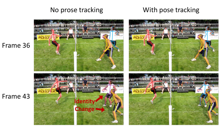
To perform human pose tracking, we follow (Umer et al. 2020) to evaluate the probability of assigning a joint to an existing or a newly appearing person. In particular, the pose tracking module considers both appearance similarities with accumulated templates, image patches for the target person in the previous frames, and the motion smoothness according to the predicted camera-centric coordinates. In Figure 10, we can see that without using pose tracking, the identity change problem is shown in the first column, while using pose tracking can fix this problem.
Failure Cases
Typical failure cases of our method are shown in Fig. 13. As our method belongs to the top-down human pose estimation approach, severe false human detection (i.e., consistently missing or duplicated) is likely to affect the performance of our method (the upper example in Fig. 13). Moreover, due to the data scarcity of 3D ground-truth (i.e., limited pose variations), our method like many others may not generalize well on wild video. In particular, as our 3D pose estimation is trained only on Human 3.6M dataset (Ionescu et al. 2014), which has limited poses variations, once unusual poses occur in the testing video (the lower example in Fig. 13), our method may not be able to generalize well.
