Gradient Coreset for Federated Learning
Abstract
Federated Learning (FL) is used to learn machine learning models with data that is partitioned across multiple clients, including resource-constrained edge devices. It is therefore important to devise solutions that are efficient in terms of compute, communication, and energy consumption, while ensuring compliance with the FL framework’s privacy requirements. Conventional approaches to these problems select a weighted subset of the training dataset, known as coreset, and learn by fitting models on it. Such coreset selection approaches are also known to be robust to data noise. However, these approaches rely on the overall statistics of the training data and are not easily extendable to the FL setup.
In this paper, we propose an algorithm called Gradient based Coreset for Robust and Efficient Federated Learning (Gcfl) that selects a coreset at each client, only every communication rounds and derives updates only from it, assuming the availability of a small validation dataset at the server. We demonstrate that our coreset selection technique is highly effective in accounting for noise in clients’ data. We conduct experiments using four real-world datasets and show that Gcfl is (1) more compute and energy efficient than FL, (2) robust to various kinds of noise in both the feature space and labels, (3) preserves the privacy of the validation dataset, and (4) introduces a small communication overhead but achieves significant gains in performance, particularly in cases when the clients’ data is noisy.
1 Introduction
Federated learning (FL) is an approach to machine learning in which clients collaborate to optimize a common objective without centralizing data [32]. The training dataset is distributed across a group of clients, and they contribute to the training process by sharing privacy-preserving updates with the central server across communication rounds until the model converges.
FL proves particularly valuable in situations where a central server lacks a sufficient amount of data for standalone model training but can leverage the collective data from multiple clients, including edge devices, sensors, or hospitals. For instance, a hospital aiming to develop a cancer prediction model can benefit from training their model using data from other hospitals, while maintaining the privacy of sensitive patient information. However, in scenarios where clients have limited computational resources or their data is noisy, it becomes imperative to design robust algorithms that enable their participation while minimizing computation and energy requirements. Our proposed solution addresses this challenge by identifying a subset of each client’s data, referred to as the ”coreset,” which reduces noise and facilitates effective training of the central server’s model.

Conventional coreset selection methods such as Facility Location, CRUST, CRAIG, Glister, and Gradmatch [34, 38, 33, 19] have been developed to enhance the efficiency and robustness of machine learning model training. However, adapting these strategies to Federated Learning (FL) settings is challenging due to the non-i.i.d. nature of clients’ datasets. Traditional coreset algorithms aim to select a representative subset that ensures a model trained on it performs similarly to the entire dataset. In FL, each client’s data originates from diverse distributions and is influenced by noise. For example, in a hospital context, data distributions differ due to varying demographics across locations and may be subject to varying amounts of different types of noise. As a result, biased updates from clients hinder the learning progress of FL algorithms. We demonstrate this obstacle through a motivating experiment in Section 2.
We introduce Gcfl (as shown in Figure 1), an algorithm specifically designed to address the aforementioned challenges. Our approach involves selecting a coreset every communication rounds to derive local updates. Similar to [49], we assume the server has access to a small validation dataset for guiding coreset selection. However, in contrast to [49], our validation dataset is not public; we exclusively use (last layer) gradients derived from it. Gcfl uses these gradients to identify a coreset at each client, effectively training the FL model. In our experiments, we demonstrate that our approach is robust to different types of noise, efficient, while preserving privacy and minimizing communication overhead111The code can be found at https://github.com/nlokeshiisc/GCFL_Release/tree/master.
In summary, our work makes the following contributions:
-
1.
We introduce Gcfl, a framework for efficiently selecting coresets for federated learning while preserving privacy.
-
2.
Through experiments, we show that Gcfl achieves the best tradeoff between accuracy and speed in a non-noisy setting.
-
3.
Furthermore, we demonstrate that Gcfl effectively filters out various types of noise, including closed-set label noise, open-set label noise, and attribute noise, resulting in improved performance compared to well-established baselines for FL and coreset selection.
2 Motivating experiment
To emphasize the need for a coreset algorithm like Gcfl in federated learning and to showcase its impact on performance, we conducted an experiment using a small toy dataset. We generated ten isotropic Gaussian blobs in with varying standard deviations (ranging from to ) using scikit-learn’s make_blob() utility [39]. A test set was reserved, containing of the samples, while the remaining training data was divided among the server and ten clients. The training subset allocated to the server serves as a validation dataset, as will be explained in our algorithm, and is solely employed to guide coreset selection at the clients.
To simulate noise, we randomly flipped of the labels in each client’s samples. We trained logistic regression models under three settings: (i) FedAvg, (ii) Gcfl, and (iii) Skyline. In the Skyline approach, clients only computed updates from the clean () samples to establish an upper-bound performance benchmark using clean data. Figure 2 displays the results, revealing that FedAvg’s performance is adversely affected by the presence of noisy training samples. In contrast, Gcfl outperforms FedAvg and falls between Skyline, demonstrating its effectiveness in mitigating the impact of noisy FL data, likely due to its use of a small, server-guided training subset. Gcfl holds significant promise for FL, especially in noisy data settings, where it significantly enhances accuracy and model generalization.
One can consider the idea of mitigating the impact of noise by fine-tuning the model refined from each communication round using the server’s validation dataset. However, such an approach may prove ineffective when the sample size in the validation dataset is insufficient. To explore this approach, we conducted experiments using CIFAR-10 and CIFAR-100 datasets, both affected by closed-set label noise. We compared the performance of Gcfl and FedAvg, as detailed in Table 1. Our observations indicate that while fine-tuning does offer some improvements, its effectiveness is limited by the small size of the validation dataset. In our upcoming experiments, we will demonstrate how Gcfl, in contrast, efficiently harnesses the validation dataset to guide coreset selection at the client side, ultimately optimizing its performance.

| Dataset | FedAvg | FedAvg + | Gcfl | Gcfl + |
|---|---|---|---|---|
| Fine Tuned | Fine Tuned | |||
| Cifar10 | 34.1% | 34.6 % | 47.4 % | 49.5 % |
| Cifar100 | 11.6% | 12.1 % | 17.5% | 17.9 % |
3 Related Work
Federated Learning (FL) is distinguished by data heterogeneity, where various clients possess data from different sources with diverse characteristics. As a result, aggregating updates from such a heterogeneous data source can impact the convergence rate of models. The challenge of addressing this heterogeneity within client data in the context of Federated Learning (FL) has garnered significant attention in the literature [12, 23, 30, 26, 15, 22].
For instance, FedProx, introduced by [26], incorporates a proximal term into the objective function. This term penalizes updates that deviate significantly from the server’s parameters, aiming to accommodate client heterogeneity. Similarly, Scaffold, proposed by [15], focuses on reducing the variance in the server’s aggregated updates by managing the drift in update computation across clients. However, FL presents a unique challenge when dealing with noisy data owned by clients, as neither the server nor the clients have a complete view of the entire training dataset. Traditional data cleaning approaches [40, 28, 9, 41] may not be directly applicable to FL.
Coreset selection is a well-established technique in machine learning that involves selecting a weighted subset of data to approximate a desired quantity across the entire dataset. Traditional coreset selection methods typically depend on the model and use submodular proxy functions for coreset selection [47, 20, 16, 10, 35]. Recent developments in the literature have explored coreset selection in conjunction with deep learning models [33, 34, 18, 5, 38]. Nevertheless, most existing coreset selection approaches are tailored for conventional settings where all data is readily accessible, requiring thoughtful adaptation for FL.
Coreset selection in Federated Learning (FL) is an underexplored domain, primarily due to the complexities tied to privacy and non-i.i.d. data distribution among clients [37, 48, 4, 36]. Notably, [1] picks a coreset of clients to collectively represent the global update across all clients using the facility location algorithm. In contrast, [37] uses Shapley values in a game-theoretic framework for again to perform client selection, while [36] explores reinforcement learning techniques for data selection. However, Nonetheless, training [36] is a challenging task, imposing an additional workload on local clients by necessitating the training of an extra private model. In comparison to the prior work, Gcfl is easy to implement and blends well with the FL framework.
4 Problem Setup
In our Federated Learning setup, a group of clients is represented by the set . The training dataset is divided among the clients, where each client has a data chunk consisting of samples . Here, denotes the input features of the data point at the client, and represents its corresponding target. It is important to note that the data chunks are disjoint, and the set of samples in each data chunk is not obtained independently and identically distributed () from the ground truth target distribution .
Our objective is to train a machine learning model where represents the learnable parameters. The server defines the objective for the downstream task and has access to a small dataset consisting of samples obtained independently and identically from the ground truth target distribution . Our aim is to minimize the expected value of the loss function , over instances sampled from the distribution .
| (1) |
As is small, it is insufficient for training and using it alone can lead to overfitting. To overcome this, the server seeks assistance from the clients to learn while respecting their privacy constraints. Federated Learning is a promising solution to this problem, where the learning progresses through communication rounds. In each round , the server selects a subset of clients and shares the current FL model parameters with them. The selected clients initialize their local model with and train it for a few epochs with their respective private data chunks to arrive at the updated model parameters . The difference in model parameters, computed as , is then transmitted back to the server. The server then averages the parameter updates received from clients and updates the FL model as follows:
| (2) |
The global learning rate used by the server is denoted as , while represents the local learning rate used by each client to train Gcfl. Although updates generated using equation (2) can minimize the objective (1) when the clients’ datasets are independently and identically distributed according to , computing updates from the entire dataset is not recommended when the data contains noise. Moreover, for resource-constrained clients such as edge devices, it is crucial to compute updates in an energy-efficient manner. To address these challenges, we propose using adaptive coreset selection, which involves selecting a weighted subset that approximates the characteristics of the entire dataset. The selected coreset should reduce computation costs without compromising the performance of the FL model, and also prevent the updates from only minimizing the client’s local loss, especially when the client’s data distribution significantly differs from the ground truth distribution . In this regard, we aim to answer the following question: How can clients in select an effective coreset that facilitates the computation of and also helps minimize the objective (1)?
5 The Gcfl Solution Approach
Let us denote the coreset selected by a client in communication round as and its associated weight as . We begin the exposition by listing certain desiderata for coreset selection in FL and then proceed to explain how Gcflmeets them.
-
1.
The algorithm should align with the current data distribution of clients while also approximating the ground truth distribution , guaranteeing a coreset that mirrors the desired target.
-
2.
The coreset algorithm should adapt and update as FL model evolves, maintaining relevance.
-
3.
Assumptions in the coreset approach should uphold FL privacy constraints, safeguarding client data and confidentiality.
To meet the first requirement, relying solely on signals from a client’s local dataset, denoted as , is insufficient, as these datasets are not identically and independently distributed with respect to the global distribution . However, contains samples drawn from the target distribution and can potentially aid in the selection of a coreset. Previous research [49] has demonstrated that making publicly accessible enables clients to choose an effective coreset. Nevertheless, in privacy-sensitive domains like healthcare, even the inclusion of may raise privacy concerns, making it unsuitable for sharing.
Hence, the task of coreset selection within the input feature space becomes challenging. As an alternative, we shift our focus towards coreset selection in the gradient space, as Federated Learning (FL) allows the server to disseminate gradients computed from . It is important to note that any cryptographic techniques applied to secure clients’ gradients, such as differential privacy, can also be employed to safeguard the server’s gradients. Additionally, to minimize communication overhead, we opt to transmit an aggregated gradient (average) derived from . This choice is grounded in the Information Bottleneck theory [43], which suggests that parameters in the final layers contain crucial discriminatory class information , while those in the initial layers primarily encapsulate feature-specific information .
We begin Gcfl by defining the server’s objective and then illustrate how we incorporate it within the Federated Learning framework. We use to signify the loss incurred by the server concerning the validation data , and denote the loss of client w.r.t. its local dataset as .
| (3) | ||||
| (4) |
where is a loss function that is pertinent to the problem.
We define as the average gradient of at on the validation dataset , and as individual data gradients of client for all . The objective for each client is to select a coreset of size such that the gradients derived from it closely match . Our coreset selection objective is:
| (5) |
Here, is a hyper-parameter that regulates the weights of selected items in the coreset. Due to the combinatorial nature of the optimization objective, it is known to be NP-Hard [19]. Therefore, we employ a greedy approximation method, which we will explain in more detail later.
Assuming that the client has solved Eq. 5, we now describe how it computes an update to share with the server. Let denote the loss on the selected coreset, defined as
| (6) |
To minimize the above loss, the client runs several epochs of stochastic gradient descent on the coreset. From the updated model, the client derives its update as follows:
| (7) |
Where is the number of local gradient update steps performed by the client on the coreset, and denotes the model parameters at the intermediate step, with . In our experiments, we observed that the coreset weight had a minimal impact on computing the update, so we omitted it in Eq (7).

5.1 Greedy solution to select Coreset (5)
Objective (5) presents a challenging combinatorial optimization problem due to the discrete variable . However, if is fixed, the inner optimization problem over weights can be addressed using the Orthogonal Matching Pursuit (OMP) algorithm, as also used in [18]. Here’s a detailed algorithm description:
The coreset selection algorithm operates iteratively, selecting points sequentially until the budget is exhausted. To illustrate, let’s consider adding the point while assuming that points have already been selected. We denote the coreset with points as and its associated weights as .
At this stage, the choice of the data point, denoted as , for inclusion in is made based on minimizing the error residue. The residue, denoted as , is computed as follows: Here, is initialized using the server’s broadcasted validation gradient . The purpose of is to quantify the remaining error that needs reduction through the addition of more points to the coreset.
We choose as , i.e., the data point that minimizes the distance between its gradient and the residue. The residue’s norm monotonically decreases with the coreset’s size increase. The pseudocode for the greedy selection is avaiable in Alg. 1 and for the overall algorithm in Alg. 2 in the Appendix.
Next, we discuss techniques to help clients implement the greedy algorithm effectively. In practice, clients can employ heuristics to avoid solving iterations to select a coreset of size by selecting multiple data points at each greedy iteration. Such an approach, backed by strong approximation guarantees, reduces the frequency of running the greedy algorithm.
To reduce computational overhead, we use the Information Bottleneck theory from [43]. This theory shows that the initial layers of deep neural networks capture input distribution, while later layers hold task-specific data. In Gcfl, the server only transmits the gradient from the softmax layer, which guides the greedy algorithm in selecting data subsets that minimize the softmax layer’s error. This strategic selection significantly trims computational costs, maintains accuracy, and reduces communication expenses by transmitting only a fraction of gradients. Moreover, the computational burden of the greedy algorithm is lessened due to the reduced dimensionality of the OMP problem.
5.2 Label-wise Coreset Selection
Here, we introduce an improved version of Gcfl for better alignment with Federated Learning. Given the data’s non-i.i.d. nature, clients often hold imbalanced class label distributions among their samples [45, 42]. Hence, a per-class coreset selection by clients is desirable. The server broadcasts gradients, each corresponding to a distinct class and derived from loss on samples . Subsequently, we execute instances of the greedy algorithm, each selecting a coreset of approximately size . Importantly, this strategy does not increase the computational overhead as the number of greedy iterations remains fixed. Furthermore, the number of gradients per Linear Regression instance within the greedy algorithm diminishes to about , which leads to a reduction in the computational requirements. However, broadcasting the server’s gradient increases communication costs by a factor of . In the following section, we delve into a simple fix to alleviate this issue.
5.3 Broadcasting Label-wise gradients
To minimize communication costs, we leverage the idea that when conducting coreset selection for a particular class , the server only needs to transmit gradients related to the penultimate layer’s connection with the output neuron for class . This approach retains the original gradient broadcast size. The label-wise coreset variant significantly trims computational expenses while maintaining communication efficiency. We present a pictorial overview of the label-wise coreset selection variant in Figure 3.
6 Experiments


We present experiments on various real world datasets with a range of noise settings to demonstrate the efficacy of Gcfl over state of the art approaches.
6.1 Datasets
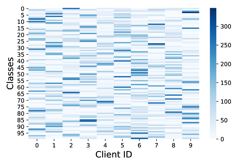
We use four datasets: CIFAR-10, CIFAR-100 [21], Flowers 222flowers: https://www.tensorflow.org/datasets/catalog/tf_flowers, and FEMNIST[3], detailed in the appendix. To replicate real-world federated learning scenarios and introduce dataset heterogeneity, we follow prior non-i.i.d. setups [44, 30]. Using a Dirichlet distribution (), we sample class proportions for clients, distributing data accordingly. We introduce attribute and label noise to showcase Gcfl’s robustness. non-i.i.d. split’s impact on dataset heterogeneity is illustrated in Figure 10(in the appendix), revealing uneven class and noise distributions across clients.
6.2 Baselines
We experiment with two kinds of baselines: coreset baselines that strive to train models with a subset of the training dataset and standard FL algorithms.
Coreset selection baselines:
-
1.
Random baseline that selects the subset randomly.
-
2.
Facility location [17] that selects a representative subset by maximising the similarity with the ground set.
- 3.
FL Algorithms with Full Dataset Updates:
-
4.
Fed-Avg [32] The popular FL algorithm that simply averages the updates and applies to the model.
-
5.
FedProx [27] Controls client drift by introducing regularization to encourage proximity to server parameters.
-
6.
Scaffold [15] Reduces variance among client updates to control drift.
-
7.
MOON [22] Uses contrastive learning to align client and server representations.
6.3 Model Architecture and Experimental Setup
We use the SGD optimizer with initial learning rates of , a momentum of , and weight decay of . We employ cosine annealing [29] to change the learning rate. The server’s model architecture consists of a two-layer CNN followed by two fully connected layers. We train models for communication rounds. During each round, coreset-based approaches process only the selected subset. We use a batch size of .
Our experiments demonstrate results that evaluate Gcfl’s robustness and efficiency. The robustness analysis compares Gcfl with baselines under different noise settings, while the efficiency evaluation considers aspects like computational and communication overhead. Ablation studies further explore Gcfl’s sensitivity to different hyperparameters.
6.4 Robustness
Standard Federated Learning methods generally struggle with noisy client data, as evident in our synthetic experiment (Figure 2). In this section, we empirically compare the robustness of Gcfl with various FL/coreset algorithms by experimenting with different noise types that exist both in attributes () and labels () and assesses their impact.
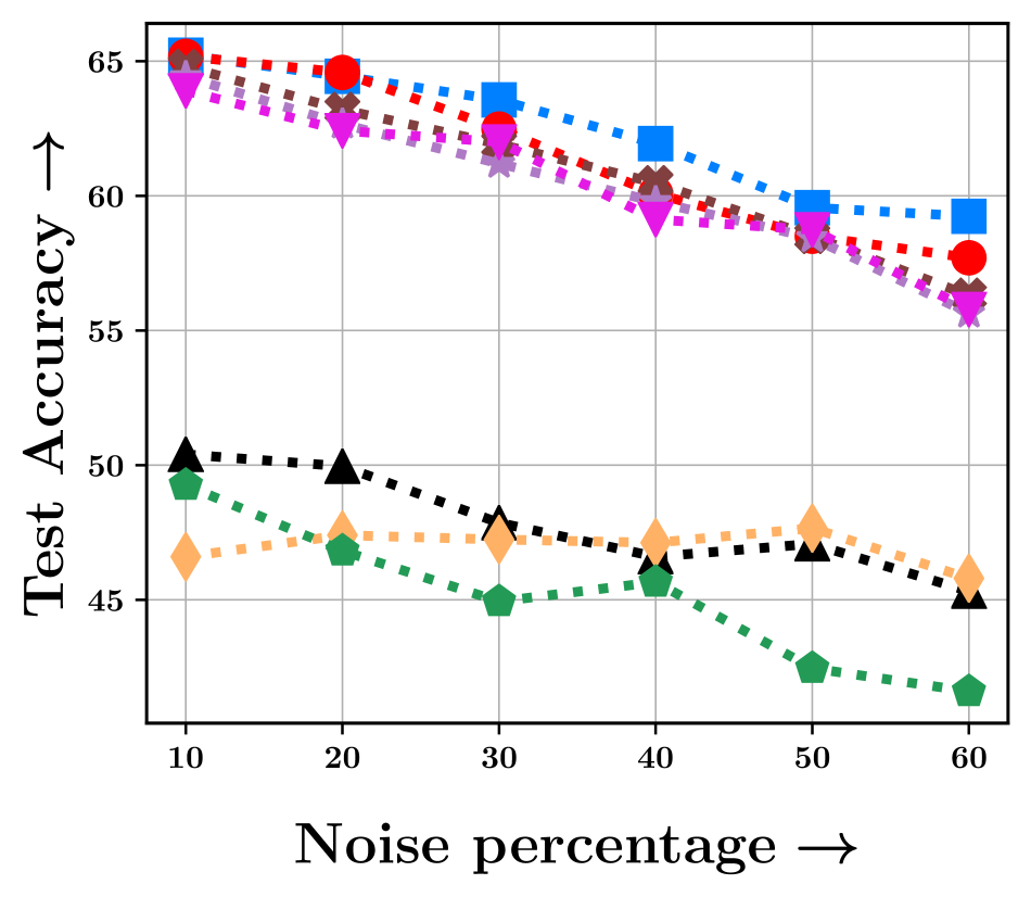
Closed Set Label noise [46]: Closed-set label noise occurs when labels in the training data are incorrect, yet they belong to the true label set . To simulate this noise with a ratio of , we randomly choose of samples from each and flip their labels. Results for closed-set noise are shown in Figure 4. Notably, Gcfl performs the best, particularly with higher noise ratios across different datasets. On the Flowers dataset, Gcfl is slightly behind Fed-Avg at lower percentages due to the dataset’s small size (only images), this dip aligns with other coreset algorithms as well.
Open Set Label Noise: [46]: Open-set label noise involves incorrect labels not belonging to the task’s label set. To simulate this with a noise ratio , we randomly mark of labels from as irrelevant. This transforms the classification task to focus on the remaining labels. We retain noisy-labeled features, but adjust their labels by flipping them to other classes, altering the task to this reduced set. Figure 5 illustrates the impact of open-set label noise on Gcfl and coreset baselines. We observe that, except for Gcfl, other coreset baselines perform worse than FedAvg baselines, primarily because identifying noisy samples is challenging without guidance from the server. For CIFAR-10, the performance improves as the percentage of open-set noise increases, when . This is due to the reduced class count, simplifying the classification task.
Attribute noise [11]: In contrast to label noise, attribute noise involves corruption of instance features. We use nine types of noise from a library333https://github.com/bethgelab/imagecorruptions to corrupt features. Figure 6 shows the effects of attribute noise. We find the Federated Learning models are relatively resilient to attribute noise. This is perhaps due to the data augmentation behavior exhibited with this kind of noise. However coreset selection methods (except Gcfl) struggle because detecting noise in attribute space without server guidance is challenging, paralleling the observation with open-set label noise.


It is evident that Gcfl outperforms other algorithms in all noise settings, as it can effectively leverage the global information providemaind by the server’s guidance to select an appropriate coreset. To further understand the reasons behind Gcfl’s superior performance, we conduct a small probing study that is outlined next.
6.5 Does Gcfl select clean data points?
In this experiment, we analyze the composition of subsets selected by various coreset selection algorithms to assess the quality of data points chosen by Gcfl. Figure 7 illustrates the noise composition in the coresets selected for CIFAR-10 and CIFAR-100 datasets under closed-set label noise. The findings demonstrate that among the subset selection algorithms, Gcfl chooses the subset with the highest count of clean points. This observation aligns with the improved performance demonstrated in Figure 4. Next, we will discuss the efficiency aspect of Gcfl and then proceed to a series of ablation studies.


6.6 Efficiency
Reducing the computational cost often involves training the models only on a subset of the dataset. The more informative the subset is, better the performance of the model. We evaluate this in Figure 8, where we compare models trained on coresets selected using different algorithms: Random, Facility Location, CRUST, and Gcfl. Due to the non-i.i.d. nature of clients datasets in FL, algorithms like CRUST and Facility Location struggle to optimize the global server objective. Moreover, adapting them to FL setup is challenging due to data privacy. Gcfl, however, aligns with the server’s last-layer loss gradient, resulting in superior performance, except for the small Flowers dataset. Figure 8 demonstrates Gcfl achieves a compelling accuracy-efficiency trade-off by just selecting coresets every rounds.
6.7 Computational overhead of Gcfl
We conducted a timing analysis on the CIFAR-10 dataset to assess Gcfl’s computational overhead. FedAvg consistently takes 1.5 seconds per round. However, Gcfl requires 5.6 seconds every round, where coreset selection is performed. In every other round, it incurs only 0.2 seconds. Therefore, for any , we would achieve significant computational benefits compared to FedAvg. For instance, with , an Gcfl epoch averages only 0.76 seconds, using just 50% of the compute compared to FedAvg.
6.8 Communication overhead of Gcfl
Gcfl introduces minimal communication overhead in practice, even though it requires transmission of validation set gradients from the server. In our experiments, the server already broadcasts the entire model with around 3.5 million parameters, while the last layer comprises only about 200 thousand parameters. As Gcfl operates every epochs (e.g., in our experiment), the long-term effect results in an additional communication overhead of merely 20 thousand parameters. This amounts to a modest increase in communication cost, keeping Gcfl’s communication cost practically equivalent to FedAvg.
6.9 Is GCFL privacy compliant?
Gcfl introduces only one additional component compared to the FedAvg, where the server broadcasts updates on to assist clients with corset selection. However, our approach requires just the softmax layer gradients. Although previous research has shown that training features can be inferred from individual data gradients, reconstructing samples with just the softmax layer gradients, particularly when averaged across instances, is exceedingly difficult. Therefore, Gcfl satisfies the privacy constraints of federated learning.


6.10 Ablation on the size of
Here, we investigate how the size of the server’s validation dataset influences the coreset selection by clients. We examine the impact by setting to represent , , and of the samples from . This analysis is conducted under conditions with both and closed-set label noise, using CIFAR10 and CIFAR100 datasets. The results, presented in Figure 9, demonstrate Gcfl’s consistent performance across varying sizes.
7 Conclusion
In this work, we introduced a new approach called Gcfl to address the challenge of learning in a federated setting where the distribution of data across the client nodes is non-i.i.d. , and ingested with noise. Our proposed approach selects a coreset from each client that best approximates the server’s last layer gradient. Our experimental results illustrate that Gcfl outperforms state-of-the-art methods, and achieves the best accuracy vs. efficiency trade-off when the datasets are not noisy. In case of noise, Gcfl was able to achieve significant gains compared to other FL and coreset selection baselines.
8 Acknowledgements
Durga Sivasubramanian and Ganesh Ramakrishnan express their gratitude to Google Research award for their assistance and funding. Ganesh Ramakrishnan is also grateful to the IIT Bombay Institute Chair Professorship for their support and sponsorship.
References
- [1] Ravikumar Balakrishnan, Tian Li, Tianyi Zhou, Nageen Himayat, Virginia Smith, and Jeff Bilmes. Diverse client selection for federated learning via submodular maximization. In International Conference on Learning Representations, 2021.
- [2] Keith Bonawitz, Vladimir Ivanov, Ben Kreuter, Antonio Marcedone, H Brendan McMahan, Sarvar Patel, Daniel Ramage, Aaron Segal, and Karn Seth. Practical secure aggregation for privacy-preserving machine learning. In proceedings of the 2017 ACM SIGSAC Conference on Computer and Communications Security, pages 1175–1191, 2017.
- [3] Sebastian Caldas, Sai Meher Karthik Duddu, Peter Wu, Tian Li, Jakub Konečnỳ, H Brendan McMahan, Virginia Smith, and Ameet Talwalkar. Leaf: A benchmark for federated settings. arXiv preprint arXiv:1812.01097, 2018.
- [4] Yae Jee Cho, Jianyu Wang, and Gauri Joshi. Client selection in federated learning: Convergence analysis and power-of-choice selection strategies. arXiv preprint arXiv:2010.01243, 2020.
- [5] Cody Coleman, Christopher Yeh, Stephen Mussmann, Baharan Mirzasoleiman, Peter Bailis, Percy Liang, Jure Leskovec, and Matei Zaharia. Selection via proxy: Efficient data selection for deep learning. In International Conference on Learning Representations, 2019.
- [6] Liam Collins, Hamed Hassani, Aryan Mokhtari, and Sanjay Shakkottai. Exploiting shared representations for personalized federated learning. In International Conference on Machine Learning, pages 2089–2099. PMLR, 2021.
- [7] Cynthia Dwork, Frank McSherry, Kobbi Nissim, and Adam Smith. Calibrating noise to sensitivity in private data analysis. In Theory of cryptography conference, pages 265–284. Springer, 2006.
- [8] Alireza Fallah, Aryan Mokhtari, and Asuman Ozdaglar. Personalized federated learning: A meta-learning approach. arXiv preprint arXiv:2002.07948, 2020.
- [9] Farzin Haddadpour and Mehrdad Mahdavi. On the convergence of local descent methods in federated learning. arXiv preprint arXiv:1910.14425, 2019.
- [10] Sariel Har-Peled and Soham Mazumdar. On coresets for k-means and k-median clustering. In Proceedings of the thirty-sixth annual ACM symposium on Theory of computing, pages 291–300, 2004.
- [11] Dan Hendrycks and Thomas Dietterich. Benchmarking neural network robustness to common corruptions and perturbations. In International Conference on Learning Representations, 2018.
- [12] Wenke Huang, Mang Ye, Bo Du, and Xiang Gao. Few-shot model agnostic federated learning. In Proceedings of the 30th ACM International Conference on Multimedia, pages 7309–7316, 2022.
- [13] Prateek Jain, John Rush, Adam Smith, Shuang Song, and Abhradeep Guha Thakurta. Differentially private model personalization. In M. Ranzato, A. Beygelzimer, Y. Dauphin, P.S. Liang, and J. Wortman Vaughan, editors, Advances in Neural Information Processing Systems, volume 34, pages 29723–29735. Curran Associates, Inc., 2021.
- [14] Peter Kairouz, Ziyu Liu, and Thomas Steinke. The distributed discrete gaussian mechanism for federated learning with secure aggregation. In International Conference on Machine Learning, pages 5201–5212. PMLR, 2021.
- [15] Sai Praneeth Karimireddy, Satyen Kale, Mehryar Mohri, Sashank Reddi, Sebastian Stich, and Ananda Theertha Suresh. Scaffold: Stochastic controlled averaging for federated learning. In International Conference on Machine Learning, pages 5132–5143. PMLR, 2020.
- [16] Vishal Kaushal, Rishabh Iyer, Suraj Kothawade, Rohan Mahadev, Khoshrav Doctor, and Ganesh Ramakrishnan. Learning from less data: A unified data subset selection and active learning framework for computer vision. In 2019 IEEE Winter Conference on Applications of Computer Vision (WACV), pages 1289–1299. IEEE, 2019.
- [17] Vishal Kaushal, Rishabh Iyer, Suraj Kothawade, Rohan Mahadev, Khoshrav Doctor, and Ganesh Ramakrishnan. Learning from less data: A unified data subset selection and active learning framework for computer vision. In 2019 IEEE Winter Conference on Applications of Computer Vision (WACV), pages 1289–1299. IEEE, 2019.
- [18] Krishnateja Killamsetty, S Durga, Ganesh Ramakrishnan, Abir De, and Rishabh Iyer. Grad-match: Gradient matching based data subset selection for efficient deep model training. In International Conference on Machine Learning, pages 5464–5474. PMLR, 2021.
- [19] Krishnateja Killamsetty, Durga Sivasubramanian, Ganesh Ramakrishnan, and Rishabh Iyer. Glister: Generalization based data subset selection for efficient and robust learning. In Proceedings of the AAAI Conference on Artificial Intelligence, volume 35, pages 8110–8118, 2021.
- [20] Katrin Kirchhoff and Jeff Bilmes. Submodularity for data selection in statistical machine translation. In Proceedings of EMNLP, pages 131–141, 2014.
- [21] Alex Krizhevsky. Learning multiple layers of features from tiny images. Technical report, 2009.
- [22] Qinbin Li, Bingsheng He, and Dawn Song. Model-contrastive federated learning. In Proceedings of the IEEE/CVF Conference on Computer Vision and Pattern Recognition, pages 10713–10722, 2021.
- [23] Qiushi Li, Wenwu Zhu, Chao Wu, Xinglin Pan, Fan Yang, Yuezhi Zhou, and Yaoxue Zhang. Invisiblefl: federated learning over non-informative intermediate updates against multimedia privacy leakages. In Proceedings of the 28th ACM International Conference on Multimedia, pages 753–762, 2020.
- [24] Shuangtong Li, Tianyi Zhou, Xinmei Tian, and Dacheng Tao. Learning to collaborate in decentralized learning of personalized models. In Proceedings of the IEEE/CVF Conference on Computer Vision and Pattern Recognition (CVPR), pages 9766–9775, June 2022.
- [25] Tian Li, Anit Kumar Sahu, Ameet Talwalkar, and Virginia Smith. Federated learning: Challenges, methods, and future directions. IEEE Signal Processing Magazine, 37(3):50–60, 2020.
- [26] Tian Li, Anit Kumar Sahu, Manzil Zaheer, Maziar Sanjabi, Ameet Talwalkar, and Virginia Smith. Federated optimization in heterogeneous networks. Proceedings of Machine Learning and Systems, 2:429–450, 2020.
- [27] Tian Li, Anit Kumar Sahu, Manzil Zaheer, Maziar Sanjabi, Ameet Talwalkar, and Virginia Smith. Federated optimization in heterogeneous networks. Proceedings of Machine Learning and Systems, 2:429–450, 2020.
- [28] Xiang Li, Kaixuan Huang, Wenhao Yang, Shusen Wang, and Zhihua Zhang. On the convergence of fedavg on non-iid data. In International Conference on Learning Representations, 2019.
- [29] Ilya Loshchilov and Frank Hutter. Sgdr: Stochastic gradient descent with warm restarts. In International Conference on Learning Representations, 2016.
- [30] Othmane Marfoq, Giovanni Neglia, Aurélien Bellet, Laetitia Kameni, and Richard Vidal. Federated multi-task learning under a mixture of distributions. Advances in Neural Information Processing Systems, 34, 2021.
- [31] Othmane Marfoq, Giovanni Neglia, Richard Vidal, and Laetitia Kameni. Personalized federated learning through local memorization. In Kamalika Chaudhuri, Stefanie Jegelka, Le Song, Csaba Szepesvari, Gang Niu, and Sivan Sabato, editors, Proceedings of the 39th International Conference on Machine Learning, volume 162 of Proceedings of Machine Learning Research, pages 15070–15092. PMLR, 17–23 Jul 2022.
- [32] Brendan McMahan, Eider Moore, Daniel Ramage, Seth Hampson, and Blaise Aguera y Arcas. Communication-efficient learning of deep networks from decentralized data. In Artificial intelligence and statistics, pages 1273–1282. PMLR, 2017.
- [33] Baharan Mirzasoleiman, Jeff Bilmes, and Jure Leskovec. Coresets for data-efficient training of machine learning models. In International Conference on Machine Learning, pages 6950–6960. PMLR, 2020.
- [34] Baharan Mirzasoleiman, Kaidi Cao, and Jure Leskovec. Coresets for robust training of deep neural networks against noisy labels. In NeurIPS, 2020.
- [35] Baharan Mirzasoleiman, Amin Karbasi, Ashwinkumar Badanidiyuru, and Andreas Krause. Distributed submodular cover: Succinctly summarizing massive data. Advances in Neural Information Processing Systems, 28, 2015.
- [36] Lokesh Nagalapatti, Ruhi Sharma Mittal, and Ramasuri Narayanam. Is your data relevant?: Dynamic selection of relevant data for federated learning. Proceedings of the AAAI Conference on Artificial Intelligence, 36(7):7859–7867, Jun. 2022.
- [37] Lokesh Nagalapatti and Ramasuri Narayanam. Game of gradients: Mitigating irrelevant clients in federated learning. In Proceedings of the AAAI Conference on Artificial Intelligence, volume 35, pages 9046–9054, 2021.
- [38] Susan Hesse Owen and Mark S Daskin. Strategic facility location: A review. European journal of operational research, 111(3):423–447, 1998.
- [39] F. Pedregosa, G. Varoquaux, A. Gramfort, V. Michel, B. Thirion, O. Grisel, M. Blondel, P. Prettenhofer, R. Weiss, V. Dubourg, J. Vanderplas, A. Passos, D. Cournapeau, M. Brucher, M. Perrot, and E. Duchesnay. Scikit-learn: Machine learning in Python. Journal of Machine Learning Research, 12:2825–2830, 2011.
- [40] Anit Kumar Sahu, Tian Li, Maziar Sanjabi, Manzil Zaheer, Ameet Talwalkar, and Virginia Smith. On the convergence of federated optimization in heterogeneous networks. arXiv preprint arXiv:1812.06127, 3:3, 2018.
- [41] Felix Sattler, Simon Wiedemann, Klaus-Robert Müller, and Wojciech Samek. Robust and communication-efficient federated learning from non-iid data. IEEE transactions on neural networks and learning systems, 31(9):3400–3413, 2019.
- [42] Zebang Shen, Juan Cervino, Hamed Hassani, and Alejandro Ribeiro. An agnostic approach to federated learning with class imbalance. In International Conference on Learning Representations, 2021.
- [43] Naftali Tishby and Noga Zaslavsky. Deep learning and the information bottleneck principle. In 2015 ieee information theory workshop (itw), pages 1–5. IEEE, 2015.
- [44] Hongyi Wang, Mikhail Yurochkin, Yuekai Sun, Dimitris Papailiopoulos, and Yasaman Khazaeni. Federated learning with matched averaging. In International Conference on Learning Representations, 2019.
- [45] Lixu Wang, Shichao Xu, Xiao Wang, and Qi Zhu. Addressing class imbalance in federated learning. In Proceedings of the AAAI Conference on Artificial Intelligence, volume 35, pages 10165–10173, 2021.
- [46] Yisen Wang, Weiyang Liu, Xingjun Ma, J. Bailey, H. Zha, L. Song, and S. Xia. Iterative learning with open-set noisy labels. 2018 IEEE/CVF Conference on Computer Vision and Pattern Recognition, pages 8688–8696, 2018.
- [47] Kai Wei, Rishabh Iyer, and Jeff Bilmes. Submodularity in data subset selection and active learning. In International Conference on Machine Learning, pages 1954–1963. PMLR, 2015.
- [48] Ruisheng Zhang, Yansheng Wang, Zimu Zhou, Ziyao Ren, Yongxin Tong, and Ke Xu. Data source selection in federated learning: A submodular optimization approach. In Database Systems for Advanced Applications: 27th International Conference, DASFAA 2022, Virtual Event, April 11–14, 2022, Proceedings, Part II, pages 606–614, 2022.
- [49] Yue Zhao, Meng Li, Liangzhen Lai, Naveen Suda, Damon Civin, and Vikas Chandra. Federated learning with non-iid data. arXiv preprint arXiv:1806.00582, 2018.
Appendix
9 Code
We have released the code in github: https://github.com/nlokeshiisc/GCFL_Release/tree/master.
10 Notation
We list the notations and their corresponding description used in Gcfl in the Table 2.
| Notation | Description |
|---|---|
| Set of clients | |
| No. of clients | |
| Training data partitioned across clients i.e. | |
| Data at each client | |
| Server’s data | |
| Subset selected at client on round and its associated weights | |
| Server loss computed on | |
| Loss at each client | |
| local learning rate at each client | |
| global learning rate at the server | |
| Denotes the number of local gradients update steps that the client performs |
11 GCFL Algorithm
Algorithm 1 presents the pseudocode of our proposed approach. The algorithm depicts the actions performed by both the server and clients at each round. The server’s actions are are highlighted in orange and the clients’ actions shown in blue color.
At a communication round , first the server samples clients (line 3), and then broadcasts to them. Additionally, if the clients need to perform coreset selection, the server also broadcasts the validation gradients. The clients subsequently use these to construct the coreset iteratively by solving our label-wise OMP problem (line of the algorithm). Then clients use the selected coreset to train the model for epochs (line 10–13). Finally, the parameters of the updated model are uploaded back to the server (line ). The server waits until it receives the updated model from all the sampled clients , then it averages them and the updates the global model with the average(line ). This completes one round of Gcfl execution.
12 Datasets Details
In table 3 we list the details about the datasets used in the experiments. Further, to showcase the challenging nature of datasets used in our experiments, we show the non-i.i.d. nature of the partition across clients using heatmaps in Figure 10. We observe that each client is characterized by an allocation of data points such that it is skewed in favor of one or two classes.
| Dataset | #Classes | #Clients’ data | #Server’s data | #Test |
|---|---|---|---|---|
| Flowers | 5 | 3270 | 200 | 200 |
| FEMNIST | 10 | 60000 | 5000 | 5000 |
| CIFAR10 | 10 | 50000 | 5000 | 5000 |
| CIFAR100 | 100 | 50000 | 5000 | 5000 |


13 Additional experiments
13.1 Client Selection


To test the robustness of Gcfl in a setting where each communication round involves partial participation of clients, we conducted an experiment by varying the number of clients that are sampled in each round. In particular, we experimented with client participation ratios , and and present the results on CIFAR10 dataset under closed-set noise setting. From the figure 11 is it clear that the robustness of Gcfl is not affected by the limited participation of clients.
13.2 Ablation study: Varying Budget
All coreset selection algorithms’ performances are affected by the size of the subset they are allowed to select. We present the effect of varying the sampling budget on coreset selection algorithms under close-set noise in Figure 12. For a fair comparison, we make the number of SGD steps consistent across different sampling budgets. For CIFAR10, in Figure 12 a) we see that Gcfl’s performance is robust to sampling budget and other coreset methods slightly improve as budget size increases. We attribute this robustness to the fact that Gcfl selects coreset based on label-wise last layer server gradients. However, for CIFAR100 dataset, in Figure 12 b) we see all the methods improve with increase in the budget size, since it is slightly a more difficult dataset having classes.


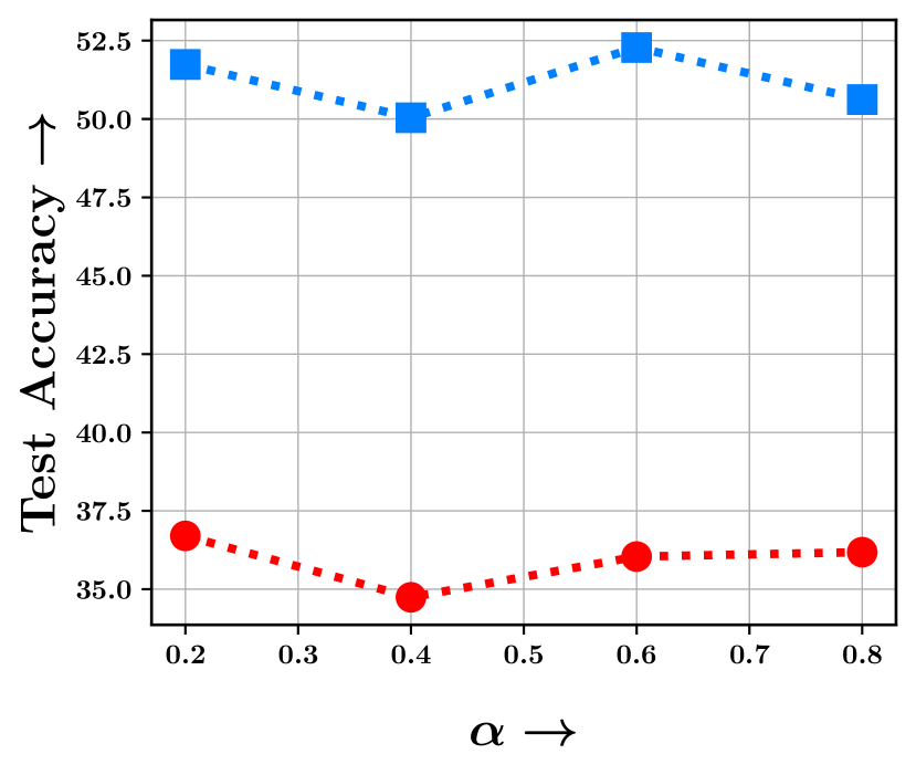
13.3 Ablation study: Varying non-i.i.d. -ness among clients
We distributed the data to clients following [30] where we simulate the non-i.i.d. data partition by sampling class proportions from a symmetric Dirichlet Distribution parameterized with . Typically, setting a lesser would result in a very skewed class proportion across clients, and as increases, we reach the uniform partition (i.e. i.i.d.) in the limit. We conduct experiments under the closed set label noise with a noise ratio of to assess the performance of Gcfl as against the standard Federated Averaging algorithm. The results are presented in Figure 13 which clearly elucidates the robustness of Gcfl primarily attributed to its ability to balance the corset across classes by deliberately running the selection on a per-class basis alongside selecting noise-free informative points. On the other hand, Federated averaging, due to its sensitivity to noise, is unable to recover even when the partition reflects i.i.d. characteristics.