Gradient Boosted Normalizing Flows

Robert Giaquinto Department of Computer Science & Engineering
University of Minnesota, Twin Cities
Minneapolis, MN 55455, USA Arindam Banerjee Department of Computer Science & Engineering
University of Minnesota, Twin Cities
Minneapolis, MN 55455, USA

Abstract

By chaining a sequence of differentiable invertible transformations, normalizing flows (NF) provide an expressive method of posterior approximation, exact density evaluation, and sampling. The trend in normalizing flow literature has been to devise deeper, more complex transformations to achieve greater flexibility. We propose an alternative: Gradient Boosted Normalizing Flows (GBNF) model a density by successively adding new NF components with gradient boosting. Under the boosting framework, each new NF component optimizes a sample weighted likelihood objective, resulting in new components that are fit to the residuals of the previously trained components. The GBNF formulation results in a mixture model structure, whose flexibility increases as more components are added. Moreover, GBNFs offer a wider, as opposed to strictly deeper, approach that improves existing NFs at the cost of additional training—not more complex transformations. We demonstrate the effectiveness of this technique for density estimation and, by coupling GBNF with a variational autoencoder, generative modeling of images. Our results show that GBNFs outperform their non-boosted analog, and, in some cases, produce better results with smaller, simpler flows.^†^†Appearing in the 34th Conference on Neural Information Processing Systems (NeurIPS 2020), Vancouver, Canada.

1 Introduction

Deep generative models seek rich latent representations of data, and provide a mechanism for sampling new data. Beyond their wide-ranging applications, generative models are an attractive class of models that place strong assumptions on the data and hence exhibit higher asymptotic bias when the model is incorrect [2]. A popular approach to generative modeling is with variational autoencoders (VAEs) [49]. A major challenge in VAEs, however, is that they assume a factorial posterior, which is widely known to limit their flexibility [66, 48, 58, 15, 42, 77, 10, 79]. Further, VAEs do not offer exact density estimation, which is a requirement in many settings.

Normalizing flows (NF) are an important recent development and can be used in both density estimation [74, 68, 20] and variational inference [66]. Normalizing flows are smooth, invertible transformations with tractable Jacobians, which can map a complex data distribution to simple distribution, such as a standard normal [61]. In the context of variational inference, a normalizing flow transforms a simple, known base distribution into a more faithful representation of the true posterior. As such, NFs complement VAEs, providing a method to overcome the limitations of a factorial posterior. Flow-based models are also an attractive approach for density estimation [74, 20, 21, 62, 19, 34, 70, 39, 41, 47, 61] because they provide exact density computation and sampling with only a single neural network pass (in some instances) [25].

Recent developments in NFs have focused of creating deeper, more complex transformations in order to increase the flexibility of the learned distribution [47, 54, 39, 12, 41, 14, 4]. With greater model complexity comes a greater risk of overfitting while slowing down training, prediction, and sampling. Boosting [28, 57, 29, 30, 31] is flexible, robust to overfitting, and generally one the most effective learning algorithms in machine learning [37]. While boosting is typically associated with regression and classification, it is also applicable in the unsupervised setting [69, 9, 58, 36, 35, 9, 53].

Our contributions.

In this work we propose a wider, as opposed to strictly deeper, approach for increasing the expressiveness of density estimators and posterior approximations. Our approach, gradient boosted normalizing flows (GBNF), iteratively adds new NF components to a model based on gradient boosting, where each new NF component is fit to the residuals of the previously trained components. A weight is learned for each component of the GBNF model, resulting in a mixture structure. However, unlike a mixture model, GBNF offers the optimality advantages associated with boosting [3], and a simplified training objective that focuses solely on optimizing a single new component at each step. GBNF compliments existing flow-based models, improving performance at the cost of additional training cycles—not more complex transformations. Prediction and sampling are not slowed with GBNF, as each component is independent and operates in parallel.

While gradient boosting is straight-forward to apply in the density estimation setting, our analysis highlights the need for analytically invertible flows in order to efficiently boost flow-based models for variational inference. Further, we address the “decoder shock” phenomenon—a challenge unique to VAEs with GBNF approximate posteriors, where the loss increases suddenly coinciding with the introduction of a new component. Our results show that GBNF improves performance on density estimation tasks, capable of modeling multi-modal data. Lastly, we augment the VAE with a GBNF variational posterior, and present image modeling results on par with state-of-the-art NFs.

The remainder of the paper is organized as follows. In Section 2 we briefly review normalizing flows. In Section 3 we introduce GBNF for density estimation, and Section 4 we extend our idea for the approximate inference setting. In Section 5 we discuss normalizing flows that are compatible with GBNF, and the “decoder shock” phenomenon. In Section 6 we present results. Finally, we conclude the paper in Section 7.

2 Background

Normalizing flows are applicable to both approximate density estimation techniques, like variational inference, as well as tractable density estimation. As such, we review variational inference techniques using modern deep neural networks to amortize the cost of learning parameters. We then share how augmenting deep generative models with normalizing flows improves variational inference. Finally, we highlight recent work using normalizing flows as density estimators directly on the data.

2.1 Variational Inference

Approximate inference plays an important role in fitting complex probabilistic models. Variational Inference (VI), in particular, transforms inference into an optimization problem with the goal of finding a variational distribution $q_{\phi}(\mathbf{z}\mid\mathbf{x})$ that closely approximates the true posterior $p(\mathbf{z}\mid\mathbf{x})$ , where $\mathbf{x}$ are the observed data, $\mathbf{z}$ the latent variables, and $\phi$ are learned parameters [45, 80, 6]. Writing the log-likelihood of the data in terms of the approximate posterior reveals:

\displaystyle\log p_{\theta}(\mathbf{x})=\underbrace{\mathbb{E}_{q_{\phi}}\left[\log\left[\frac{p_{\theta}(\mathbf{x},\mathbf{z})}{q_{\phi}(\mathbf{z}\mid\mathbf{x})}\right]\right]}_{\mathcal{L}_{\theta,\phi}(\mathbf{x})\quad\text{(ELBO)}}+\underbrace{\mathbb{E}_{q_{\phi}}\left[\log\left[\frac{q_{\phi}(\mathbf{z}\mid\mathbf{x})}{p_{\theta}(\mathbf{z}\mid\mathbf{x})}\right]\right]}_{KL(q_{\phi}(\mathbf{z}\mid\mathbf{x})\,||\,p_{\theta}(\mathbf{z}\mid\mathbf{x}))}

(1)

Since the second term in (1) is the Kullback-Leibler (KL) divergence, which is non-negative, then the first term forms a lower bound on the log-likelihood of the data, and hence referred to as the evidence lower bound (ELBO).

2.2 Variational Autoencoder

Kingma and Welling, [49], Rezende et al., [67] show that a re-parameterization of the ELBO can result in a differentiable bound that is amenable to optimization via stochastic gradients and back-propagation. Further, Kingma and Welling, [49] structure the inference problem as an autoencoder, introducing the variational autoencoder (VAE) and minimizing the negative-ELBO $\mathcal{F}_{\phi,\theta}^{(VI)}(\mathbf{x})$ . Re-writing the VI objective $\mathcal{F}_{\phi,\theta}^{(VI)}(\mathbf{x})$ as:

\mathcal{F}_{\phi,\theta}^{(VI)}(\mathbf{x})=\mathbb{E}_{q_{\phi}}\left[-\log p_{\theta}(\mathbf{x}\mid\mathbf{z})\right]+KL\left(q_{\phi}(\mathbf{z}\mid\mathbf{x})\,||\,p(\mathbf{z})\right)~{},

(2)

shows the probabilistic decoder $p_{\theta}(\mathbf{x}\mid\mathbf{z})$ , and highlights how the VAE encodes the latent variables $\mathbf{z}$ with the variational posterior $q_{\phi}(\mathbf{z}\mid\mathbf{x})$ , but $q_{\phi}(\mathbf{z}\mid\mathbf{x})$ is regularized with the prior $p(\mathbf{z})$ .

2.3 Normalizing Flows

Tabak and Vanden-Eijnden, [75], Tabak and Turner, [74] introduce normalizing flows (NF) as a composition of simple maps. Parameterizing flows with deep neural networks [21, 20, 68] has popularized the technique for density estimation and variational inference [61].

Variational Inference

Rezende and Mohamed, [66] use NFs to modify the VAE’s [49] posterior approximation $q_{0}$ by applying a chain of $K$ transformations $\mathbf{z}_{K}=f_{K}\circ\dots\circ f_{1}(\mathbf{z}_{0})$ to the inference network output $\mathbf{z}_{0}\sim q_{0}(\mathbf{z}_{0}\mid\mathbf{x})$ . By defining $f_{k},k=1,\ldots,K$ as an invertible, smooth mapping, by the chain rule and inverse function theorem $z_{k}=f_{k}(z_{k-1})$ has a computable density [75, 74]:

\displaystyle q_{k}(\mathbf{z}_{k})=q_{k-1}(\mathbf{z}_{k-1})\left|\det\frac{\partial f_{k}^{-1}}{\partial\mathbf{z}_{k-1}}\right|=q_{k-1}(\mathbf{z}_{k-1})\left|\det\frac{\partial f_{k}}{\partial\mathbf{z}_{k-1}}\right|^{-1}~{}.

(3)

Thus, a VAE with a $K$ -step flow-based posterior minimizes the negative-ELBO:

\displaystyle\mathcal{F}_{\theta,\phi}^{(VI)}(\mathbf{x})

\displaystyle=\mathbb{E}_{q_{0}}\left[-\log p_{\theta}(\mathbf{x}\mid\mathbf{z}_{K})-\sum_{k=1}^{K}\log\left|\det\frac{\partial f_{k}}{\partial\mathbf{z}_{k-1}}\right|\right]+KL\left(q_{0}(\mathbf{z}_{0}\mid\mathbf{x})\,||\,p(\mathbf{z}_{K})\right)~{},

(4)

where $q_{0}(\mathbf{z}_{0}\mid\mathbf{x})$ is a known base distribution (e.g. standard normal) with parameters $\phi$ .

Density Estimation

Given a set of samples $\{\mathbf{x}_{i}\}_{i=1}^{n}$ from a target distribution $p^{*}$ , our goal is to learn a flow-based model $p_{\phi}(\mathbf{x})$ , which corresponds to minimizing the forward KL-divergence: $\mathcal{F}^{(ML)}(\phi)=KL(p^{*}(\mathbf{x})\,||\,p_{\phi}(\mathbf{x}))$ [61]. A NF formulates $p_{\phi}(\mathbf{x})$ as a transformation $\mathbf{x}=f(\mathbf{z})$ of a base density $p_{0}(\mathbf{z})$ with $f=f_{K}\circ\dots\circ f_{1}$ as a $K$ -step flow [20, 21, 62]. Thus, to estimate the expectation over $p^{*}$ we take a Monte Carlo approximation of the forward KL, yielding:

\displaystyle\mathcal{F}^{(ML)}(\phi)

\displaystyle\approx-\frac{1}{n}\sum_{i=1}^{n}\left[\log p_{0}\left(f^{-1}(\mathbf{x}_{i})\right)+\sum_{k=1}^{K}\log\left|\det\frac{\partial f_{k}^{-1}}{\partial\mathbf{x}_{i}}\right|\right]~{},

(5)

which is equivalent to fitting the model to samples $\{\mathbf{x}_{i}\}_{i=1}^{n}$ by maximum likelihood estimation [61].

2.4 Gradient Boosting

Gradient boosting [57, 29, 30, 31] considers the minimization of a loss $\mathcal{F}(G)$ , where $G(\cdot)$ is a function representing the current model. Consider an additive perturbation around $G$ to $G+\epsilon g$ , where $g$ is a function representing a new component. A Taylor expansion as $\epsilon\rightarrow 0$ :

\mathcal{F}(G+\epsilon g)=\mathcal{F}(G)+\epsilon\langle g,\nabla\mathcal{F}(G)\rangle+o(\epsilon^{2})~{},

(6)

reveals the functional gradient $\nabla\mathcal{F}(G)$ , which is the direction that reduces the loss at the current solution.

Thus, to minimize loss $\mathcal{F}(G)$ at the current model, choose the best function $g$ in a class of functions $\mathcal{G}$ (e.g. regression trees), which corresponds to solving a linear program where $\nabla\mathcal{F}(G)$ defines the weights for every function in $\mathcal{G}$ . Underlying Gradient boosting is a connection to conditional gradient descent and the Frank-Wolfe algorithm [26]: we first solve a constrained convex minimization problem to choose $g$ , then solve a line-search problem to appropriately weight $g$ relative to the previous components $G$ [9, 36].

3 Density Estimation with GBNF

Gradient boosted normalizing flows (GBNF) build on recent ideas in boosting for variational inference [36, 58] and generative models [35] in order to increase the flexibility of density estimators and posteriors approximated with NFs. A GBNF is constructed by successively adding new components based on forward-stagewise gradient boosting, where each new component $g^{(c)}_{K}$ is a $K$ -step normalizing flow that is fit to the functional gradient of the loss from the $(c-1)$ previously trained components $G^{(c-1)}_{K}$ .

Gradient boosting assigns a weight $\rho_{c}$ to the new component $g^{(c)}_{K}$ and we restrict $\rho_{c}\in[0,1]$ to ensure the model stays a valid probability distribution. The resulting density can be written as a mixture model:

\displaystyle G_{K}^{(c)}(\mathbf{x})

\displaystyle=\psi\left((1-\rho_{c})\psi^{-1}(G_{K}^{(c-1)}(\mathbf{x}))+\rho_{c}\psi^{-1}(g_{K}^{(c)}(\mathbf{x}))\right)/\Gamma_{(c)}~{},

(7)

where the full model $G_{K}^{(c)}(\mathbf{x})$ is a monotonic function $\psi$ of a convex combination of fixed components $G_{K}^{(c-1)}$ and new component $g_{K}^{(c)}$ , and $\Gamma_{(c)}$ is the partition function. Two special cases are of interest: first, when $\psi(a)=a$ , which corresponds to a standard additive mixture model with $\Gamma_{(c)}=1$ :

\displaystyle\log G_{K}^{(c)}(\mathbf{x})

\displaystyle=\log\left((1-\rho_{c})(G_{K}^{(c-1)}(\mathbf{x}))+\rho_{c}(g_{K}^{(c)}(\mathbf{x}))\right)~{}.

Second, when $\psi(a)=\exp(a)$ with $\psi^{-1}(a)=\log(a)$ , which corresponds to a multiplicative mixture model [35, 17]:

\displaystyle\log G_{K}^{(c)}(\mathbf{x})

\displaystyle=\left((1-\rho_{c})\log(G_{K}^{(c-1)}(\mathbf{x}))+\rho_{c}\log(g_{K}^{(c)}(\mathbf{x}))\right)-\log\Gamma_{(c)}~{}.

The advantage of GBNF over a standard mixture model with a pre-determined fixed number of components is that additional components can always be added to the model, and the weights $\rho_{c}$ for non-informative components will degrade to zero. Since each GBNF component is a NF, we evaluate (7) recursively, and at each stage the last component is computed by the change of variables formula:

g_{K}^{(c)}=p_{0}\left(f_{c}^{-1}(\mathbf{x})\right)\prod_{k=1}^{K}\left|\det\frac{\partial f^{-1}_{k,c}}{\partial\mathbf{x}}\right|~{},

(8)

where $f_{c}=f_{c,K}\circ\cdots\circ f_{c,1}$ is the $K$ -step flow transformation for component $c$ , and the base density $p_{0}$ is shared by all components. In our formulation we consider $c$ components, where $c$ is fixed and finite.

Density Estimation

With GBNF density estimation is similar to (5): we seek flow parameters $\boldsymbol{\phi}=[\phi_{1},\dots,\phi_{c}]$ that minimize $KL\left(p^{*}(\mathbf{x})\,||\,G_{K}^{(c)}(\mathbf{x})\right)$ , which for finite number of samples $\{\mathbf{x}_{i}\}$ drawn from $p^{*}(\mathbf{x})$ corresponds to minimizing:

\mathcal{F}^{(ML)}(\boldsymbol{\phi})=-\frac{1}{n}\sum_{i=1}^{n}\left[\log\left\{\psi\left((1-\rho_{c})\psi^{-1}(G_{K}^{(c-1)}(\mathbf{x}_{i}))+\rho_{c}\psi^{-1}(g_{K}^{(c)}(\mathbf{x}_{i}))\right)/\Gamma_{(c)}\right\}\right]~{}.

(9)

Directly optimizing (9) for mixture model $G_{K}^{(c)}$ is non-trivial. Gradient boosting, however, provides an elegant solution that greatly simplifies the problem. During training, the first component is fit using a traditional objective function—no boosting is applied²²2No boosting during the first stage is equivalent to setting $G^{(0)}_{K}(\mathbf{x})$ to uniform on the domain of $\mathbf{x}$ .. At stages $c>1$ , we already have $G_{K}^{(c-1)}$ , consisting of a convex combination of the $(c-1)$ $K$ -step flow models from the previous stages, and we train a new component $g_{K}^{(c)}$ by taking a Frank-Wolfe [26, 5, 9, 43, 53, 36] linear approximation of the loss (9). Since jointly optimizing w.r.t. both $g_{K}^{(c)}$ and $\rho_{c}$ is a challenging non-convex problem [36], we train $g_{K}^{(c)}$ until convergence, and then use (9) as the objective to optimize w.r.t the corresponding weight $\rho_{c}$ .

3.1 Updates to New Boosting Components

Additive Boosting

We first consider the special case $\psi(a)=a$ and $\Gamma_{(c)}=1$ , corresponding to the additive mixture model. Our goal is to derive an update to the new component $g_{K}^{(c)}$ using functional gradient descent. Thus, we take the gradient of (9) w.r.t. fixed parameters $\boldsymbol{\phi}_{1:c-1}$ of $G_{K}^{(c)}$ at $\rho_{c}\rightarrow 0$ , giving:

\displaystyle\nabla_{\boldsymbol{\phi}_{1:c-1}}\mathcal{F}^{(ML)}(\boldsymbol{\phi})\Big{|}_{\rho_{c}\rightarrow 0}

\displaystyle=-\frac{1-\rho_{c}}{(1-\rho_{c})G_{K}^{(c-1)}+\rho_{c}g_{K}^{(c)}}\Bigg{|}_{\rho_{c}\rightarrow 0}=-\frac{1}{G_{K}^{(c-1)}}

(10)

Since $G_{K}^{(c-1)}$ is fixed, then maximizing $-\mathcal{F}^{(ML)}(\boldsymbol{\phi})$ is achieved by choosing a new component $g_{K}^{(c)}$ and weighing by the negative of the gradient from (10) over the samples:

\displaystyle g_{K}^{(c)}

\displaystyle=\operatorname*{arg\,max}_{g_{K}\in\mathcal{G}_{K}}\frac{1}{n}\sum_{i=1}^{n}\frac{g_{K}(\mathbf{x}_{i})}{G_{K}^{(c-1)}(\mathbf{x}_{i})}~{},

(11)

where $\mathcal{G}_{K}$ is the family of $K$ -step flows. Note that (11) is a linear program in which $G_{K}^{(c-1)}(\mathbf{x}_{i})$ is a constant, and will hence yield a degenerate point probability distribution where the entire probability mass is placed at the minimum point of $G_{K}^{(c-1)}$ . To avoided the degenerate solution, a standard approach adds an entropy regularization term which is controlled by the hyperparameter $\lambda$ [36, 9]:

\displaystyle g_{K}^{(c)}

\displaystyle=\operatorname*{arg\,max}_{g_{K}\in\mathcal{G}_{K}}\frac{1}{n}\sum_{i=1}^{n}\frac{g_{K}(\mathbf{x}_{i})}{G_{K}^{(c-1)}(\mathbf{x}_{i})}-\lambda\sum_{i=1}^{n}g_{K}(\mathbf{x}_{i})\log g_{K}(\mathbf{x}_{i})~{}.

(12)

Multiplicative Boosting

In this paper, we instead use $\psi(a)=\exp(a)$ with $\psi^{-1}(a)=\log(a)$ , which corresponds to the multiplicative mixture model, and, from the boosting perspective, a multiplicative boosting model [35, 17]. However, in contrast to the existing literature on multiplicative boosting for probabilistic models, we consider boosting with normalizing flow components. In the multiplicative setting, explicitly maintaining the convex combination between $G_{K}^{(c-1)}$ and $g_{K}^{(c)}$ is unnecessary: the partition function $\Gamma_{(c)}$ ensures the validity of the probabilistic model. Thus, the multiplicative GBNF seeks a new component $g_{K}^{(c)}$ that minimizes:

\mathcal{F}^{(ML)}(\boldsymbol{\phi})=-\frac{1}{n}\sum_{i=1}^{n}\left[\left(\log(G_{K}^{(c-1)}(\mathbf{x}_{i}))+\rho_{c}\log(g_{K}^{(c)}(\mathbf{x}_{i}))\right)-\log\Gamma_{(c)}\right]~{}.

(13)

The partition function is defined as $\Gamma_{(c)}=\int_{x}\prod_{j=1}^{c}(g_{K}^{(j)})^{\rho_{j}}(\mathbf{x})p_{0}(\mathbf{x})d\mathbf{x}$ and computing $\Gamma_{(c)}$ for GBNF is straightforward since normalizing flows learn self-normalized distributions—and hence can be computed without resorting to simulated annealing or Markov chains [35]. Moreover, following standard properties [35, 17], we also inherit a recursive property of the partition function. To see the recursive property, denote the un-normalized GBNF density as $\tilde{G}_{K}^{(c)}$ , where $\tilde{G}_{K}^{(c)}\propto G_{K}^{(c)}$ but $\tilde{G}_{K}^{(c)}$ does not integrate to $1$ . Then, by definition:

\Gamma_{(c)}G_{K}^{(c)}(\mathbf{x})=g_{K}^{(c)}(\mathbf{x})^{\rho_{c}}\tilde{G}_{K}^{(c-1)}(\mathbf{x})=\Gamma_{(c-1)}g_{K}^{(c)}(\mathbf{x})^{\rho_{c}}G_{K}^{(c-1)}(\mathbf{x})~{},

then, integrating both sides and using $\int_{\mathbf{x}}G_{K}^{(c)}(\mathbf{x})d\mathbf{x}=1$ gives

\Gamma_{(c)}=\Gamma_{(c-1)}\int_{\mathbf{x}}g_{K}^{(c)}(\mathbf{x})^{\rho_{c}}G_{K}^{(c-1)}(\mathbf{x})d\mathbf{x}=\Gamma_{(c-1)}\mathbb{E}_{G_{K}^{(c-1)}}\left[g_{K}^{(c)}(\mathbf{x})^{\rho_{c}}\right]~{}.

and therefore $\Gamma_{(c)}=\Gamma_{(c-1)}\mathbb{E}_{G_{K}^{(c-1)}}[g_{K}^{(c)}(\mathbf{x})^{\rho_{c}}]$ , as desired.

The objective in (13) represents the loss under the model $G_{K}^{(c)}$ which followed from minimizing the forward KL-divergence $KL(p^{*}\|\mathbf{G}_{K}^{(c)})$ , where $\mathbf{G}_{K}^{(c)}$ is the normalized approximate distribution and $p^{*}$ the target distribution. To improve (13) with gradient boosting, consider the difference in losses after introducing a new component $g_{K}^{(c)}$ to the model:

$\displaystyle KL(p^{}\\|\mathbf{G}_{K}^{(c-1)})-KL(p^{}\\|\mathbf{G}_{K}^{(c)})$	$\displaystyle=\mathbb{E}_{p^{}}\left[\log\frac{p^{}(\mathbf{x})}{G_{K}^{(c-1)}(\mathbf{x})}-\log\frac{p^{*}(\mathbf{x})}{G_{K}^{(c)}(\mathbf{x})}\right]$
	$\displaystyle=\mathbb{E}_{p^{*}}\left[\log\frac{G_{K}^{(c)}(\mathbf{x})}{G_{K}^{(c-1)}(\mathbf{x})}\right]$
	$\displaystyle=\mathbb{E}_{p^{*}}\left[\log\frac{(g_{K}^{(c)}(\mathbf{x}))^{\rho_{c}}\tilde{G}_{K}^{(c-1)}(\mathbf{x})}{\Gamma_{c-1}\mathbb{E}_{G_{K}^{(c-1)}}[(g_{K}^{(c)}(\mathbf{x}))^{\rho_{c}}]}\times\frac{\Gamma_{c-1}}{\tilde{G}_{K}^{(c-1)}(\mathbf{x})}\right]$
	$\displaystyle=\mathbb{E}_{p^{*}}\left[\log\frac{(g_{K}^{(c)}(\mathbf{x}))^{\rho_{c}}}{\mathbb{E}_{G_{K}^{(c-1)}}[(g_{K}^{(c)}(\mathbf{x}))^{\rho_{c}}]}\right]$
	$\displaystyle=\mathbb{E}_{p^{*}}\left[\log g_{K}^{(c)}(\mathbf{x}))^{\rho_{c}}\right]-\log\mathbb{E}_{G_{K}^{(c-1)}}\left[g_{K}^{(c)}(\mathbf{x}))^{\rho_{c}}\right]$
	$\displaystyle\stackrel{{\scriptstyle(a)}}{{\geq}}\mathbb{E}_{p^{*}}\left[\log g_{K}^{(c)}(\mathbf{x}))^{\rho_{c}}\right]-\log\left(\mathbb{E}_{G_{K}^{(c-1)}}[g_{K}^{(c)}(\mathbf{x})]\right)^{\rho_{c}}$
	$\displaystyle=\rho_{c}\left\{\mathbb{E}_{p^{*}}\left[\log g_{K}^{(c)}(\mathbf{x})\right]-\log\mathbb{E}_{G_{K}^{(c-1)}}\left[g_{K}^{(c)}(\mathbf{x})\right]\right\}~{},$	(14)

where (a) follows by Jensen’s inequality since $\rho_{c}\in[0,1]$ . Note that we want to choose the new component $g_{K}^{(c)}(\mathbf{x})$ so that $KL(p^{*}\|\mathbf{G}_{K}^{(c)})$ is minimized, or equivalently, for a fixed $\mathbf{G}_{K}^{(c-1)}$ , the difference $KL(p^{*}\|\mathbf{G}_{K}^{(c-1)})-KL(p^{*}\|\mathbf{G}_{K}^{(c)})$ is maximized. Since $\rho_{c}\geq 0$ , it suffices to focus on the following maximization problem:

g_{K}^{(c)}=\operatorname*{arg\,max}_{g_{K}\in\mathcal{G}_{K}}~{}\mathbb{E}_{p^{*}}\left[\log g_{K}(\mathbf{x})\right]-\log\mathbb{E}_{G_{K}^{(c-1)}}\left[g_{K}(\mathbf{x})\right]~{}.

(15)

If we choose a new component according to:

g_{K}^{(c)}(\mathbf{x})=\frac{p^{*}(\mathbf{x})}{G_{K}^{(c-1)}(\mathbf{x})}~{},

then, with this choice of $g_{K}^{(c)}$ , we see that (15) reduces to:

\mathbb{E}_{p^{*}}\left[\log\frac{p^{*}(\mathbf{x})}{G_{K}^{(c-1)}(\mathbf{x})}\right]-\log\mathbb{E}_{G_{K}^{(c-1)}}\left[\frac{p^{*}(\mathbf{x})}{G_{K}^{(c-1)}(\mathbf{x})}\right]=KL\left(p^{*}\|\mathbf{G}_{K}^{(c-1)}\right)-\underbrace{\log\mathbb{E}_{p^{*}(\mathbf{x})}\left[1\right]}_{0}~{}.

Our choice of $g_{K}^{(c)}$ is, therefore, optimal and gives a lower bound to (3.1) with $KL(p^{*}\|\mathbf{G}_{K}^{(c)})\rightarrow 0$ . The solution to (15) can also be understood in terms of the change-of-measure inequality [1, 23], which also forms the basis of the PAC-Bayes bound and a certain regret bounds [1].

Similar to the additive case, the new component chosen in (15) shows that $g_{K}^{(c)}$ maximizes the likelihood of the samples while discounting those that are already explained by $G_{K}^{(c-1)}$ . Unlike the additive GBNF update in (12), however, the multiplicative GBNF update is a numerically stable and does not require an entropy regularization term.

Further, our analysis reveals the source of a surrogate loss function [59, 3, 60] which optimizes the global objective—namely, when written as as a minimization (15) is the weighted negative log-likelihood of the samples. Surrogate loss functions are common in the boosting framework [28, 71, 3, 29, 27, 8, 76, 69]. Adaboost [27, 28], in particular, solves a re-weighted classification problem where weak learners, in the form of decision trees, optimize surrogate losses like information gain or Gini index. The negative log-likelihood is specifically chosen as a surrogate loss function in other boosted probabilistic and density estimation models which also have $f$ -divergence based global objectives [35, 69], however here we clarify that the surrogate loss follows from (3.1).

In practice, instead of weighing the loss by to the reciprocal of the fixed components, we follow Grover and Ermon, [35] and train the new component to perform maximum likelihood estimation over a re-weighted data distribution:

\displaystyle g_{K}^{(c)}=\operatorname*{arg\,min}_{g_{K}\in\mathcal{G}_{K}}\,\mathop{\mathbb{E}}_{\mathcal{D}^{(c-1)}}\left[-\log g_{K}\right]

(16)

where $\mathcal{D}^{(c-1)}$ denotes a re-weighted data distribution whose samples are drawn with replacement using sample weights inversely-proportional to $G_{K}^{(c-1)}$ . Since (16) is the same objective as the generative multiplicative boosting model in Grover and Ermon, [35], where we have set their parameter $\beta$ from Proposition 1 to one, then (16) provides a non-increasing update to the multiplicative objective function (13).

Lastly, we note that the analysis of Cranko and Nock, [17] highlights important properties of the broader class of boosted density estimation models that optimize (9), of which both the additive and multiplicative forms of GBNF are members. Specifically, Remark 3 in Cranko and Nock, [17] shows a sharper decrease in the loss—that is, for any step size $\rho\in[0,1]$ the loss has geometric convergence:

\displaystyle KL\left(p^{*}\,||\,\mathbf{G}_{K}^{(c)}|\rho_{c}\right)\leq(1-\rho_{c})KL\left(p^{*}\,||\,\mathbf{G}_{K}^{(c-1)}\right)

(17)

where $\mathbf{G}_{K}^{(c)}|\rho_{c}$ denotes the explicit dependence of $\mathbf{G}_{K}^{(c)}(\mathbf{x})$ on $\rho_{c}$ . Thus GBNF provides a strong convergence guarantee on the global objective.

3.2 Update to Component Weights

Component weights $\rho$ are updated to satisfy $\rho_{c}=\operatorname*{arg\,min}_{\rho}\mathcal{F}^{(ML)}(\boldsymbol{\phi})$ using line-search. Alternatively, taking the gradient of the loss $\mathcal{F}_{\boldsymbol{\phi}}^{(ML)}(\mathbf{x})$ with respect to $\rho_{c}$ gives a stochastic gradient descent (SGD) algorithm (see Section 4.2, for example).

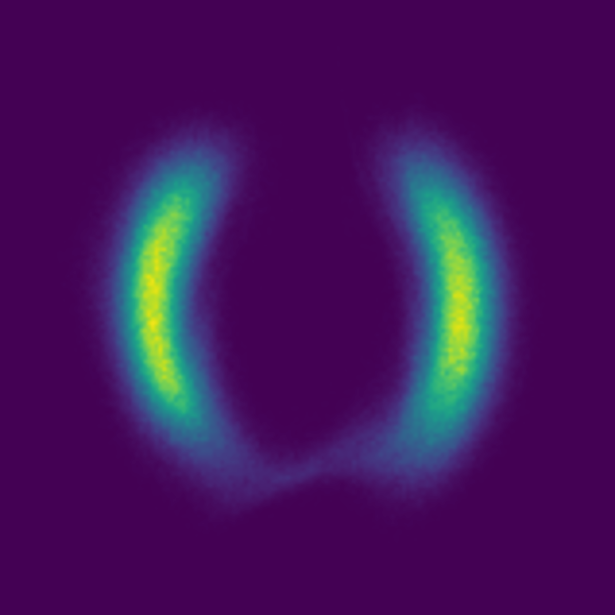
Updating a component’s weight is only needed once after each component converges. We find, however, that results improve by “fine-tuning” each component and their weights with additional training after the initial training pass. During the fine-tuning stage, we sequentially retrain each component $g_{K}^{(i)}$ for $i=1,\dots,c$ , during which we treat $G_{K}^{(-i)}$ as fixed where $-i$ represents the mixture of all other components: $1,\dots,i-1,i+1,\dots c$ . Figure 1 demonstrates this phenomenon: when a single flow is not flexible enough to model the target, mode-covering behavior arises. Introducing the second component trained with the boosting objective improves results, and consequently the second component’s weight is increased. Fine-tuning the first component leads to a better solution and assigns equal weight to the two components.

4 Variational Inference with GBNF

Gradient boosting is also applicable to posterior approximation with flow-based models. For variational inference we map a simple base distribution to a complex posterior. Unlike (4), however, we consider a VAE whose approximate posterior $G_{K}^{(c)}$ is a GBNF with $c$ components and of the form:

G_{K}^{(c)}(\mathbf{z}\mid\mathbf{x})=(1-\rho_{c})G_{K}^{(c-1)}(\mathbf{z}\mid\mathbf{x})+\rho_{c}g_{K}^{(c)}(\mathbf{z}\mid\mathbf{x})~{}.

(18)

We seek a variational posterior that closely matches the true posterior $p(\mathbf{z}\mid\mathbf{x})$ , which corresponds to the reverse KL-divergence $KL(G_{K}^{(c)}(\mathbf{z}\mid\mathbf{x})\,||\,p(\mathbf{z}\mid\mathbf{x}))$ . Minimizing KL is equivalent to minimizing $\mathcal{F}_{\phi,\theta}^{(VI)}(\mathbf{x})$ the negative-ELBO up to a constant. Thus, we seek to minimize the variational bound:

\mathcal{F}_{\phi,\theta}^{(VI)}(\mathbf{x})=\mathbb{E}_{G_{K}^{(c)}}\left[\log G_{K}^{(c)}(\mathbf{z}_{K}\mid\mathbf{x})-\log p_{\theta}(\mathbf{x},\mathbf{z}_{K})\right]~{}.\\

(19)

4.1 Updates to New Boosting Components

Given the bound (19), we then derive updates for new components. Similar to Section 3.1, consider the functional gradient w.r.t. $G_{K}^{(c)}$ at $\rho_{c}\rightarrow 0$ :

\nabla_{G_{K}^{(c)}}\mathcal{F}_{\phi,\theta}^{(VI)}(\mathbf{x})\big{|}_{\rho_{c}\rightarrow 0}=-\log\frac{p_{\theta}(\mathbf{x},\mathbf{z})}{G_{K}^{(c-1)}(\mathbf{z}\mid\mathbf{x})}

(20)

We minimize $\mathcal{F}_{\theta,\phi}^{(VI)}(\mathbf{x})$ by choosing a new component $g_{K}^{(c)}$ that has the minimum inner product with the gradient from (20).

\displaystyle g_{K}^{(c)}

\displaystyle=\operatorname*{arg\,min}_{g_{K}\in{\cal G}_{K}}~{}\sum_{i=1}^{n}\mathop{\mathbb{E}}_{g_{K}(\mathbf{z}\mid\mathbf{x}_{i})}\left[\nabla_{G}\mathcal{F}(\mathbf{x}_{i})\right]

However, to avoid $g_{K}^{(c)}$ degenerating to a point mass at the functional gradient’s minimum, we add an entropy regularization term³³3In our experiments that augment the VAE with a GBF-based posterior, we find good results setting the regularization $\lambda=1.0$ . In the density estimation experiments, better results are often achieved with $\lambda$ near 0.8. controlled by $\lambda>0$ , thus:

g_{K}^{(c)}=\operatorname*{arg\,min}_{g_{K}\in{\cal G}_{K}}\sum_{i=1}^{n}\mathop{\mathbb{E}}_{g_{K}(\mathbf{z}\mid\mathbf{x}_{i})}\left[\nabla_{G}\mathcal{F}(\mathbf{x}_{i})+\lambda\log g_{K}(\mathbf{z}\mid\mathbf{x}_{i})\right].

(21)

Despite the differences in derivation, optimization of GBNF has a similar structure to other flow-based VAEs. Specifically, with the addition of the entropy regularization, rearranging (21) shows:

g_{K}^{(c)}=\operatorname*{arg\,min}_{g_{K}\in{\cal G}_{K}}\mathop{\mathbb{E}}_{g_{K}(\mathbf{z}\mid\mathbf{x})}\left[-\log\frac{p_{\theta}(\mathbf{x}\mid\mathbf{z}_{K}^{(c)})}{G_{K}^{(c-1)}(\mathbf{z}_{K}^{(c)}\mid\mathbf{x})}\right]+KL\left(\lambda g_{K}(\mathbf{z}_{K}^{(c)}\mid\mathbf{x})\,||\,p(\mathbf{z}_{K}^{(c)})\right)~{}.

(22)

If $G_{K}^{(c-1)}$ is constant, then we recover the VAE objective exactly. By learning a GBNF approximate posterior the reconstruction error – $\log p_{\theta}(\mathbf{x}\mid\mathbf{z}_{K}^{(c)})$ is down-weighted for samples that are easily explained by the fixed components. For updates to the component weights $\rho$ see Appendix 4.2.

Lastly, we note that during a forward pass the model encodes data to produce $\mathbf{z}_{0}$ . To sample from the posterior $\mathbf{z}_{K}\sim G_{K}^{(c)}$ , however, we transform $\mathbf{z}_{0}$ according to $\mathbf{z}_{K}=f_{K}^{(j)}\circ\dots\circ f_{1}^{(j)}(\mathbf{z}_{0})$ , where $j\sim Categorical(\rho)$ randomly chooses a component—similar to sampling from a mixture model. Thus, during training we compute a fast stochastic approximation of the likelihood $G_{K}^{(c)}$ . Likewise, prediction and sampling are as fast as the non-boosted setting, and easily parallelizable across components.

4.2 Updating Component Weights

Let: Tolerance

\epsilon>0

, and Step-size

\delta>0

Initialize weight

\rho_{c}^{(0)}=1/C

Set iteration

t=0

while $|\rho_{c}^{(t)}-\rho_{c}^{(t-1)}|<\epsilon$ do

Draw mini-batch samples

\mathbf{z}_{K,i}^{(c-1)}\sim G_{K}^{(c-1)}(\mathbf{z}\mid\mathbf{x}_{i})

and

\mathbf{z}_{K,i}^{(c)}\sim g_{K}^{(c)}(\mathbf{z}\mid\mathbf{x}_{i})

for

i=1,\dots,n

Compute Monte Carlo estimate of gradient

\nabla_{\rho_{c}}\mathcal{F}_{\theta,\phi}^{(VI)}(\mathbf{x})=\frac{1}{n}\sum_{i=1}^{n}\gamma_{\rho_{c}}^{(t-1)}(\mathbf{z}_{K,i}^{(c)}\mid\mathbf{x}_{i})-\gamma_{\rho_{c}}^{(t-1)}(\mathbf{z}_{K,i}^{(c-1)}\mid\mathbf{x}_{i})

t = t + 1

\rho_{c}^{(t)}=\rho_{c}^{(t-1)}-\delta\nabla_{\rho_{c}}

\rho_{c}^{(t)}=

clip

(\rho_{c}^{(t)},[0,1])

return

\rho_{c}^{(t)}

Algorithm 1 Updating Mixture Weight

\rho_{c}

After $g_{K}^{(c)}(\mathbf{z}_{K}\mid\mathbf{x})$ has been estimated, the mixture model still needs to estimate $\rho_{c}\in[0,1]$ . Similar to the density estimation setting, the weights on each component can be updated by taking the gradient of the loss $\mathcal{F}_{\phi,\theta}^{(VI)}(\mathbf{x})$ with respect to $\rho_{c}$ . Recall that $G_{K}^{(c)}(\mathbf{z}_{K}\mid\mathbf{x})$ can be written as the convex combination:

	$\displaystyle G_{K}^{(c)}(\mathbf{z}_{K}\mid\mathbf{x})=$	$\displaystyle(1-\rho_{c})G_{K}^{(c-1)}(\mathbf{z}_{K}\mid\mathbf{x})+\rho_{c}g_{K}^{(c)}(\mathbf{z}_{K}\mid\mathbf{x})$
		$\displaystyle=\rho_{c}\left(g_{K}^{(c)}(\mathbf{z}_{K}\mid\mathbf{x})-G_{K}^{(c-1)}(\mathbf{z}_{K}\mid\mathbf{x})\right)+G_{K}^{(c-1)}(\mathbf{z}_{K}\mid\mathbf{x})~{},$

Then, with $\Delta_{K}^{(c)}(\mathbf{z}_{K}\mid\mathbf{x})\triangleq g_{K}^{(c)}(\mathbf{z}_{K}\mid\mathbf{x}_{i})-G_{K}^{(c-1)}(\mathbf{z}_{K}\mid\mathbf{x}_{i})$ , the objective function $\mathcal{F}_{\theta,\phi}^{(VI)}(\mathbf{x})$ can be written as a function of $\rho_{c}$ :

	$\displaystyle\mathcal{F}_{\theta,\phi}^{(VI)}(\mathbf{x})$	$\displaystyle=\sum_{i=1}^{n}\left\langle\rho_{c}\Delta_{K}^{(c)}(\mathbf{z}_{K}\mid\mathbf{x}_{i})+G_{K}^{(c-1)}(\mathbf{z}_{K}\mid\mathbf{x}_{i}),-\log p_{\theta}(\mathbf{x}_{i},\mathbf{z}_{K})\right\rangle$
		$\displaystyle+\sum_{i=1}^{n}\bigg{\langle}\rho_{c}\Delta_{K}^{(c)}(\mathbf{z}_{K}\mid\mathbf{x}_{i})+G_{K}^{(c-1)}(\mathbf{z}_{K}\mid\mathbf{x}_{i}),\log\left(\rho_{c}\Delta_{K}^{(c)}(\mathbf{z}_{K}\mid\mathbf{x}_{i})+G_{K}^{(c-1)}(\mathbf{z}_{K}\mid\mathbf{x}_{i})\right)\bigg{\rangle}~{}.$		(23)

The above expression can be used in a black-box line search method or, as we have done, in a stochastic gradient descent algorithm 1. Toward that end, taking gradient of (4.2) w.r.t. $\rho_{c}$ yields the component weight updates:

\displaystyle\frac{\partial\mathcal{F}_{\phi,\theta}^{(VI)}}{\partial\rho_{c}}=\sum_{i=1}^{n}

\displaystyle\left(\mathop{\mathbb{E}}_{g_{K}^{(c)}(\mathbf{z}\mid\mathbf{x}_{i})}\left[\gamma_{\rho_{c}}^{(t-1)}(\mathbf{z}\mid\mathbf{x}_{i})\right]-\mathop{\mathbb{E}}_{G_{K}^{(c-1)}(\mathbf{z}\mid\mathbf{x}_{i})}\left[\gamma_{\rho_{c}}^{(t-1)}(\mathbf{z}\mid\mathbf{x}_{i})\right]\right)~{},

(24)

where we’ve defined:

\displaystyle\gamma_{\rho_{c}}^{(t-1)}(\mathbf{z}\mid\mathbf{x}_{i})\triangleq\log\left(\frac{(1-\rho_{c}^{(t-1)})G_{K}^{(c-1)}(\mathbf{z}\mid\mathbf{x}_{i})+\rho_{c}^{(t-1)}g_{K}^{(c)}(\mathbf{z}\mid\mathbf{x}_{i})}{p_{\theta}(\mathbf{x}_{i},\mathbf{z})}\right)~{}.

To ensure a stable convergence we follow Guo et al., [36] and implement an SGD algorithm with a decaying learning rate.

4.3 Decoder Shock: Abrupt Changes to the VAE Approximate Posterior

Sharing the decoder between all GBNF components presents a unique challenge in training a VAE with a GBNF approximate posterior. During training the decoder acclimates to samples from a particular component (e.g. $g^{(old)}$ ). However, when a new stage begins the decoder begins receiving samples from a new component $g^{(new)}$ . At this point the loss jumps (see Figure 2), a phenomenon we refer to as “decoder shock”. Reasons for “decoder shock” are as follows.

The introduction of $g^{(new)}$ causes a sudden shift in the distribution of samples passed to the decoder, causing a sharp increase in reconstruction errors. Further, we anneal the KL [7, 73, 38] in (22) cyclically [32], with restarts corresponding to the introduction of new boosting components. By reducing the weight of the KL term in (22) during the initial epochs the model is free to discover useful representations of the data before being penalized for complexity. Without KL-annealing, models may choose the “low hanging fruit” of ignoring $\mathbf{z}$ and relying purely on a powerful decoder [7, 73, 15, 65, 18, 38]. Thus, when the annealing schedule restarts, $g^{(new)}$ is unrestricted and the validation’s KL term temporarily increases.

A spike in loss between boosting stages is unique to GBNF. Unlike other boosted models, with GBNF there is a module (the decoder) that depends on the boosted components—this does not exist when boosting decision trees for regression or classification (for example). To overcome the “decoder shock” problem, propose a simple solution that deviates from a traditional boosting approach. Instead of only drawing samples from $g_{K}^{(c)}$ during training, we periodically sample from the fixed components, helping the decoder remember past components and adjust to changes in the full approximate posterior $G_{K}^{(c)}$ . We emphasize that despite drawing samples from $G_{K}^{(c-1)}$ , the parameters for $G_{K}^{(c-1)}$ remain fixed—samples from $G_{K}^{(c-1)}$ are purely for the decoder’s benefit. Additionally, Figure 2 highlights how fine-tuning (blue line) consolidates information from all components and improves results at very little computational cost.

5 Related Work

Below we highlight connections between GBNF and related work, along with unique aspects of GBNF. First, we discuss the catalog of normalizing flows that are compatible with gradient boosting. We then compare GBNF to other boosted generative models and flows with mixture formulations.

Flows Compatible with Gradient Boosting

While all normalizing flows can be boosted for density estimation, boosting for variational inference is only practical with analytically invertible flows (see Figure 3). The focus of GBNF for variational inference is on training the new component $g_{K}^{(c)}$ , but in order to draw samples $\mathbf{z}_{K}^{(c)}\sim g_{K}^{(c)}$ we sample from the base distribution $\mathbf{z}_{0}\sim q_{0}(\mathbf{z}\mid\mathbf{x})$ and transform $\mathbf{z}_{0}$ according to:

\mathbf{z}_{K}^{(c)}=f_{c,K}\circ\dots\circ f_{c,2}\circ f_{c,1}(\mathbf{z}_{0})~{}.

However, updating $g_{K}^{(c)}$ for variational inference requires computing the likelihood $G_{K}^{(c-1)}(\mathbf{z}_{K}^{(c)}\mid\mathbf{x})$ . Following Figure 3, to compute $G_{K}^{(c-1)}$ we seek the point $\tilde{\mathbf{z}}_{0}$ within the base distribution such that:

\mathbf{z}_{K}^{(c)}=f_{K}^{(j)}\circ\dots\circ f_{2}^{(j)}\circ f_{1}^{(j)}(\tilde{\mathbf{z}}_{0})~{},

where $\mathbf{z}_{K}^{(c)}$ is sampled from $g^{(c)}$ and $j\sim Categorical(\rho_{1:c-1})$ randomly chooses one of the fixed components. Then, under the change of variables formula, we approximate $G_{K}^{(c-1)}(\mathbf{z}_{K}^{(c)}\mid\mathbf{x})$ by:

q_{0}(\tilde{\mathbf{z}}_{0})\prod_{k=1}^{K}\left|\det\frac{\partial f_{k}^{(j)}}{\partial\tilde{\mathbf{z}}_{k-1}}\right|^{-1}.

While planar and radial [66], Sylvester [79], and neural autoregressive flows [41, 19] are provably invertible, we cannot compute the inverse. Inverse and masked autoregressive flows [48, 62] are invertible, but $D$ times slower to invert where $D$ is the dimensionality of $\mathbf{z}$ .

Analytically invertible flows include those based on coupling layers, such as NICE [20], RealNVP [21], and Glow—which replaced RealNVP’s permutation operation with a $1\times 1$ convolution [47]. Neural spline flows increase the flexibility of both coupling and autoregressive transforms using monotonic rational-quadratic splines [25], and non-linear squared flows [81] are highly multi-modal and can be inverted for boosting. Continuous-time flows [11, 13, 34, 70] use transformations described by ordinary differential equations, with FFJORD being “one-pass” invertible by solving an ODE.

Flows with Mixture Formulations

The main bottleneck in creating more expressive flows lies in the base distribution and the class of transformation function [61]. Autoregressive [41, 44, 19, 48, 62, 54], residual [4, 14, 79, 66], and coupling-layer flows [20, 21, 47, 39, 64] are the most common classes of finite transformations, however, discrete (RAD, [22]) and continuous (CIF, [16]) mixture formulations offer a promising new approach where the base distribution and transformation change according to the mixture component. GBNF also presents a mixture formulation, but trained in a different way, where only the updates to the newest component are needed during training and extending an existing model with additional components is trivial. Moreover, GBNF optimizes a different objective that fits new components to the residuals of previously trained components, which can refine the mode covering behavior of VAEs (see Hu et al., [40]) and maximum likelihood (similar to Dinh et al., [22]). The continuous mixture approach of CIF, however, cannot be used in the variational inference setting to augment the VAE’s approximate posterior [16].

Gradient Boosted Generative Models

By considering convex combinations of distributions $G$ and $g$ , boosting is applicable beyond the traditional supervised setting [9, 17, 35, 36, 52, 53, 69, 76]. In particular, boosting variational inference (BVI, [58, 36, 17]) improves a variational posterior, and boosted generative models (BGM, [35]) constructs a density estimator by iteratively combining sum-product networks. Unlike BVI and BGM our approach addresses the unique algorithmic challenges of boosting applied to flow-based models—such as the need for analytically invertible flows and the “decoder shock” phenomena when enhancing the VAE’s approximate posterior with GBNF.

6 Experiments

To evaluate GBNF, we highlight results on two toy problems, density estimation on real data, and boosted flows within a VAE for generative modeling of images. We boost coupling flows [21, 47] parameterized by feed-forward networks with TanH activations and a single hidden layer. While RealNVP [21], in particular, is less flexible and shown to be empirically inferior to planar flows in variational inference [66], coupling flows are attractive for boosting: sampling and inference require one forward pass, log-likelihoods are computed exactly, and they are trivially invertible. In the toy experiments flows are trained for 25k iterations using the Adam optimizer [46]. For all other experiments details on the datasets and hyperparameters can be found in Appendix A.

6.1 Toy Density Matching

For density matching the model generates samples from a standard normal and transforms them into a complex distribution $p_{X}$ . The 2-dimensional unnormalized target’s analytical form $p^{*}$ is known and parameters are learned by minimizing $KL(p_{X}\,||\,p^{*})$ .

Results

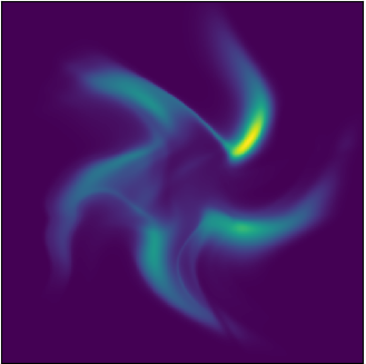
In Figure 4 we compare our results to a deep 16-step RealNVP flow on four energy functions. In each case GBNF provides an accurate density estimation with half as many parameters. When the component flows are flexible enough to model most or all of the target density, components can overlap. However, by training the component weights $\rho$ the model down-weights components that don’t provide additional information. On more challenging targets, such as 3 (top-right), GBNF fits one component to each of the top and bottom divergences within the energy function, and some component overlap occurring elsewhere.

6.2 Toy Density Estimation

We apply GBNF to the density estimation problems found in [47, 34, 19]. Here the model receives samples from an unknown 2-dimensional data distribution, and the goal is to learn a density estimator of the data. We consider GBNF with either $c=4$ or $8$ RealNVP components, each of which includes $K=1,2,4,$ or $8$ coupling layers [21], respectively. Here RealNVP and GBNF use flows of equivalent depth, and we evaluate improvements resulting from GBNF’s additional boosted components.

Results

As shown in Figure 5, even when individual components are weak the composite model is expressive. For example, the 8-Gaussians figure shows that the first component (RealNVP column) fails to model all modes. With additional 1-step flows, GNBF achieves a multimodal density model. Both the 8-Gaussians and Spiral results show that adding boosted components can drastically improve density estimates without requiring more complex transformations. On the Checkerboard and Pinwheel, where RealNVP matches the data more closely, GBNF sharpens density estimates.

6.3 Density Estimation on Real Data

Following Grathwohl et al., [34] we report density estimation results on the POWER, GAS, HEPMASS, and MINIBOONE datasets from the UCI machine learning repository [24], as well as the BSDS300 dataset [56]. We compare boosted and non-boosted RealNVP [21] and Glow models [47]. Glow uses a learned base distribution, whereas our boosted implementation of Glow (and the RealNVPs) use fixed Gaussians. Results for non-boosted models are from [34].

Results

In Table 1 we find significant improvements by boosting Glow and the more simple RealNVP normalizing flows, even with only $c=4$ components. Our implementation of Glow was unable to match the results for BSDS300 from [34], and only achieves an average log-likelihood of 152.96 without boosting. After boosting Glow with $c=4$ components, however, the log-likelihood rises significantly to 154.68, which is comparable to the baseline.

Table 1: Log-likelihood on the test set (higher is better) for 4 datasets from UCI machine learning [24] and BSDS300 [56]. Here

d

is the dimensionality of data-points and

n

the size of the dataset. GBNF models include

c=4

components. Mean/stdev are estimated over 3 runs.

Model	POWER $\uparrow$	GAS $\uparrow$	HEPMASS $\uparrow$	MINIBOONE $\uparrow$	BSDS300 $\uparrow$
Model	$d$ =6; $n$ =2,049,280	$d$ =8; $n$ =1,052,065	$d$ =21; $n$ =525,123	$d$ =43; $n$ =36,488	$d$ =63; $n$ =1,300,000
RealNVP	$0.17$ $\pm.01$	$8.33$ $\pm.14$	$-18.71$ $\pm.02$	$-13.55$ $\pm.49$	$153.28$ $\pm 1.78$
Boosted RealNVP	$0.27$ $\pm 0.01$	$9.58$ $\pm.04$	$-18.60$ $\pm 0.06$	$-10.69$ $\pm 0.07$	$154.23$ $\pm 2.21$
Glow	$0.17$ $\pm.01$	$8.15$ $\pm.40$	$-18.92$ $\pm.08$	$-11.35$ $\pm.07$	$155.07$ $\pm.03$
Boosted Glow	$0.24$ $\pm 0.01$	$9.95$ $\pm 0.11$	$-17.81$ $\pm 0.12$	$-10.76$ $\pm 0.02$	$154.68$ $\pm 0.34$

6.4 Image Modeling with Variational Autoencoders

Following Rezende and Mohamed, [66], we employ NFs for improving the VAE’s approximate posterior [49]. We compare our model on the same image datasets as those used in van den Berg et al., [79]: Freyfaces, Caltech 101 Silhouettes [55], Omniglot [50], and statically binarized MNIST [51].

Results

In Table 2 we compare the performance of GBNF to other normalizing flow architectures. In all results RealNVP, which is more ideally suited for density estimation tasks, performs the worst of the flow models. Nonetheless, applying gradient boosting to RealNVP improves the results significantly. On Freyfaces, the smallest dataset consisting of just 1965 images, gradient boosted RealNVP gives the best performance—suggesting that GBNF may avoid overfitting. For the larger Omniglot dataset of hand-written characters, Sylvester flows are superior, however, gradient boosting improves the RealNVP baseline considerably and is comparable to Sylvester. GBNF improves on the baseline RealNVP, however both GBNF and IAF’s results are notably higher than the non-coupling flows on the Caltech 101 Silhouettes dataset. Lastly, on MNIST we find that boosting improves NLL on RealNVP, and is on par with Sylvester flows. All models have an approximately equal number of parameters, except the baseline VAE (fewer parameters) and Sylvester which has $\approx 5$ x the number of parameters (grid search for hyperparameters is chosen following [79]).

Table 2: Negative ELBO (lower is better) and Negative log-likelihood (NLL, lower is better) results on MNIST, Freyfaces, Omniglot, and Caltech 101 Silhouettes datasets. For the Freyfaces dataset the results are reported in bits per dim. Results for the other datasets are reported in nats. GBNF models include

c=4

RealNVP components. The top 3 NLL results for each dataset are in bold.

Model	MNIST		Freyfaces		Omniglot		Caltech 101
Model	-ELBO $\downarrow$	NLL $\downarrow$	-ELBO $\downarrow$	NLL $\downarrow$	-ELBO $\downarrow$	NLL $\downarrow$	-ELBO $\downarrow$	NLL $\downarrow$
VAE	$89.32$ $\pm 0.07$	$84.97$ $\pm 0.01$	$4.84$ $\pm 0.07$	$4.78$ $\pm 0.07$	$109.77$ $\pm 0.06$	$103.16$ $\pm 0.01$	$120.98$ $\pm 1.07$	$108.43$ $\pm 1.81$
Planar	$86.47$ $\pm 0.09$	$83.16$ $\pm 0.07$	$4.64$ $\pm 0.04$	4.60 $\pm 0.04$	$105.72$ $\pm 0.08$	100.18 $\pm 0.01$	$116.70$ $\pm 1.70$	104.23 $\pm 1.60$
Radial	$88.43$ $\pm 0.07$	$84.32$ $\pm 0.06$	$4.73$ $\pm 0.08$	$4.68$ $\pm 0.07$	$108.74$ $\pm 0.57$	$102.07$ $\pm 0.50$	$118.89$ $\pm 1.30$	$106.88$ $\pm 1.55$
Sylvester	84.54 $\pm 0.01$	81.99 $\pm 0.02$	4.54 $\pm 0.03$	4.49 $\pm 0.03$	101.99 $\pm 0.23$	98.54 $\pm 0.29$	112.26 $\pm 2.01$	100.38 $\pm 1.20$
IAF	$86.46$ $\pm 0.07$	83.14 $\pm 0.06$	$4.73$ $\pm 0.04$	$4.70$ $\pm 0.05$	$106.34$ $\pm 0.14$	$100.97$ $\pm 0.07$	$119.62$ $\pm 0.84$	$108.41$ $\pm 1.31$
RealNVP	$88.04$ $\pm 0.07$	$83.36$ $\pm 0.09$	$4.66$ $\pm 0.17$	$4.62$ $\pm 0.16$	$106.22$ $\pm 0.59$	$100.43$ $\pm 0.19$	$123.26$ $\pm 2.06$	$113.00$ $\pm 1.70$
GBNF	$87.00$ $\pm 0.16$	82.59 $\pm 0.03$	$4.49$ $\pm 0.01$	4.41 $\pm 0.01$	$105.60$ $\pm 0.20$	99.09 $\pm 0.17$	$121.41$ $\pm 0.71$	106.40 $\pm 0.54$

7 Conclusion

In this work we introduce gradient boosted normalizing flows, a technique for increasing the flexibility of flow-based models through gradient boosting. GBNF, iteratively adds new NF components, where each new component is fit to the residuals of the previously trained components. We show that GBNF can improve results for existing normalizing flows on density estimation and variational inference tasks. In our experiments we demonstrated that GBNF improves over their baseline single component model, without increasing the depth of the model, and produces image modeling results on par with state-of-the-art flows. Further, we showed GBNF models used for density estimation create more flexible distributions at the cost of additional training and not more complex transformations.

In the future we wish to further investigate the “decoder shock” phenomenon occurring when GBNF is paired with a VAE. Future work may benefit from exploring other strategies for alleviating “decoder shock”, such as multiple decoders or different annealing strategies. In our real data experiments in Section 6.4 we fixed the entropy regularization $\lambda$ at 1.0, however adjusting the regularization on a per-component level may be worth pursuing. Additionally, in our image modeling experiments we used RealNVP as the base component. Future work may consider other flows for boosting, as well as heterogeneous combinations of flows as the different components.

8 Broader Impact

As a generative model, gradient boosted normalizing flows (GBNF) are suited for a variety of tasks, including the synthesis of new data-points. A primary motivation for choosing GBNF, in particular, is producing a flexible model that can synthesize new data-points quickly. GBNF’s individual components can be less complex and thus faster, yet as a whole the model is powerful. Since the components operate in parallel, prediction and sampling can be done quickly—a valuable characteristic for deployment on mobile devices. One limitation of GBNF is the requirement for additional computing resources to train the added components, which can be costly for deep flow-based models. As such, GBNF advantages research laboratories and businesses with access to scalable computing. Those with limited computing resources may find benchmarking or deploying GBNF too costly.

Acknowledgements

The research was supported by NSF grants OAC-1934634, IIS-1908104, IIS-1563950, IIS-1447566, IIS-1447574, IIS-1422557, CCF-1451986. We thank the University of Minnesota Supercomputing Institute (MSI) for technical support.

References

Banerjee, [2006] Banerjee, A. (2006). On bayesian bounds. In Proceedings of the 23rd International Conference on Machine Learning, pages 81–88. ACM.
Banerjee, [2007] Banerjee, A. (2007). An Analysis of Logistic Models: Exponential Family Connections and Online Performance. In Proceedings of the 2007 SIAM International Conference on Data Mining, Proceedings, pages 204–215. Society for Industrial and Applied Mathematics.
Bartlett et al., [2006] Bartlett, P. L., Jordan, M. I., and McAuliffe, J. D. (2006). Convexity, Classification, and Risk Bounds. Journal of the American Statistical Association, 101(473):138–156.
Behrmann et al., [2019] Behrmann, J., Grathwohl, W., Chen, R. T. Q., Duvenaud, D., and Jacobsen, J.-H. (2019). Invertible Residual Networks. In International Conference on Machine Learning, page 10.
Beygelzimer et al., [2015] Beygelzimer, A., Hazan, E., Kale, S., and Luo, H. (2015). Online Gradient Boosting. In Advances in Neural Information Processing Systems, page 9.
Blei et al., [2017] Blei, D. M., Kucukelbir, A., and McAuliffe, J. D. (2017). Variational Inference: A Review for Statisticians. Journal of the American Statistical Association, 112(518):859–877.
Bowman et al., [2016] Bowman, S. R., Vilnis, L., Vinyals, O., Dai, A., Jozefowicz, R., and Bengio, S. (2016). Generating Sentences from a Continuous Space. In Proceedings of The 20th SIGNLL Conference on Computational Natural Language Learning, pages 10–21, Berlin, Germany. Association for Computational Linguistics.
Bühlmann and Hothorn, [2007] Bühlmann, P. and Hothorn, T. (2007). Boosting Algorithms: Regularization, Prediction and Model Fitting. Statistical Science, 22(4):477–505.
Campbell and Li, [2019] Campbell, T. and Li, X. (2019). Universal Boosting Variational Inference. In Advances in Neural Information Processing Systems.
Casale et al., [2018] Casale, F. P., Dalca, A. V., Saglietti, L., Listgarten, J., and Fusi, N. (2018). Gaussian Process Prior Variational Autoencoders. Advances in Neural Information Processing Systems, page 11.
[11] Chen, C., Li, C., Chen, L., Wang, W., Pu, Y., and Carin, L. (2017a). Continuous-Time Flows for Efficient Inference and Density Estimation. arXiv:1709.01179 [stat].
Chen et al., [2020] Chen, J., Lu, C., Chenli, B., Zhu, J., and Tian, T. (2020). VFlow: More Expressive Generative Flows with Variational Data Augmentation. arXiv:2002.09741 [cs, stat].
Chen et al., [2018] Chen, R. T. Q., Rubanova, Y., Bettencourt, J., and Duvenaud, D. (2018). Neural Ordinary Differential Equations. In Advances in Neural Information Processing Systems.
Chen et al., [2019] Chen, T. Q., Behrmann, J., Duvenaud, D. K., and Jacobsen, J.-H. (2019). Residual Flows for Invertible Generative Modeling. In Advances in Neural Information Processing Systems, page 11.
[15] Chen, X., Kingma, D. P., Salimans, T., Duan, Y., Dhariwal, P., Schulman, J., Sutskever, I., and Abbeel, P. (2017b). Variational Lossy Autoencoder. ICLR.
Cornish et al., [2020] Cornish, R., Caterini, A. L., Deligiannidis, G., and Doucet, A. (2020). Relaxing Bijectivity Constraints with Continuously Indexed Normalising Flows. arXiv:1909.13833 [cs, stat].
Cranko and Nock, [2019] Cranko, Z. and Nock, R. (2019). Boosting Density Estimation Remastered. Proceedings of the 36th International Conference on Machine Learning, 97:1416–1425.
Cremer et al., [2018] Cremer, C., Li, X., and Duvenaud, D. (2018). Inference Suboptimality in Variational Autoencoders. In International Conference on Machine Learning, Stockholm, Sweden.
De Cao et al., [2019] De Cao, N., Titov, I., and Aziz, W. (2019). Block Neural Autoregressive Flow. 35th Conference on Uncertainty in Artificial Intelligence (UAI19).
Dinh et al., [2015] Dinh, L., Krueger, D., and Bengio, Y. (2015). NICE: Non-linear Independent Components Estimation. ICLR.
Dinh et al., [2017] Dinh, L., Sohl-Dickstein, J., and Bengio, S. (2017). Density estimation using Real NVP. ICLR.
Dinh et al., [2019] Dinh, L., Sohl-Dickstein, J., Pascanu, R., and Larochelle, H. (2019). A RAD approach to deep mixture models. arXiv:1903.07714 [cs, stat].
Donsker and Varadhan, [1976] Donsker, M. D. and Varadhan, S. R. S. (1976). On the principal eigenvalue of second-order elliptic differential operators. Communications on Pure and Applied Mathematics, 29(6):595–621.
Dua and Taniskidou, [2017] Dua, D. and Taniskidou, E. K. (2017). UCI Machine Learning Repository. https://archive.ics.uci.edu/ml/index.php.
Durkan et al., [2019] Durkan, C., Bekasov, A., Murray, I., and Papamakarios, G. (2019). Neural Spline Flows. In Advances in Neural Information Processing Systems.
Frank and Wolfe, [1956] Frank, M. and Wolfe, P. (1956). An Algorithm for Quadratic Programming. Naval Research Logistics Quarterly, 3:95–110.
Freund and Schapire, [1996] Freund, Y. and Schapire, R. E. (1996). Experiments with a New Boosting Algorithm. In International Conference on Machine Learning, page 9.
Freund and Schapire, [1997] Freund, Y. and Schapire, R. E. (1997). A Decision-Theoretic Generalization of On-Line Learning and an Application to Boosting. Journal of Computer and System Sciences, 55(1):119–139.
Friedman et al., [2000] Friedman, J., Hastie, T., and Tibshirani, R. (2000). Additive logistic regression: A statistical view of boosting. The annals of statistics, 28(2):337–407.
Friedman, [2001] Friedman, J. H. (2001). Greedy function approximation: A gradient boosting machine. Annals of statistics, pages 1189–1232.
Friedman, [2002] Friedman, J. H. (2002). Stochastic gradient boosting. Computational Statistics & Data Analysis, 38(4):367–378.
Fu et al., [2019] Fu, H., Li, C., Liu, X., Gao, J., Celikyilmaz, A., and Carin, L. (2019). Cyclical Annealing Schedule: A Simple Approach to Mitigating KL Vanishing. In NAACL.
Germain et al., [2015] Germain, M., Gregor, K., Murray, I., and Larochelle, H. (2015). MADE: Masked Autoencoder for Distribution Estimation. In International Conference on Machine Learning, volume 37, Lille, France.
Grathwohl et al., [2019] Grathwohl, W., Chen, R. T. Q., Bettencourt, J., Sutskever, I., and Duvenaud, D. (2019). FFJORD: Free-form Continuous Dynamics for Scalable Reversible Generative Models. In International Conference on Learning Representations.
Grover and Ermon, [2018] Grover, A. and Ermon, S. (2018). Boosted Generative Models. In AAAI.
Guo et al., [2016] Guo, F., Wang, X., Fan, K., Broderick, T., and Dunson, D. B. (2016). Boosting Variational Inference. In Advances in Neural Information Processing Systems, Barcelona, Spain.
Hastie et al., [2001] Hastie, T., Tibshirani, R., and Friedman, J. (2001). The Elements of Statistical Learning, volume 1 of Springer Series in Statistics. Springer New York Inc., second edition.
Higgins et al., [2017] Higgins, I., Matthey, L., Pal, A., Burgess, C., Glorot, X., Botvinick, M., Mohamed, S., and Lerchner, A. (2017). $\beta$ -VAE: Learning Basic Visual Concepts with a Constrained Variational Framework. ICLR, page 22.
Ho et al., [2019] Ho, J., Chen, X., Srinivas, A., Duan, Y., and Abbeel, P. (2019). Flow++: Improving Flow-Based Generative Models with Variational Dequantization and Architecture Design. In International Conference on Machine Learning.
Hu et al., [2018] Hu, Z., Yang, Z., Salakhutdinov, R., and Xing, E. P. (2018). On Unifying Deep Generative Models. In ICLR, pages 1–19.
[41] Huang, C.-W., Krueger, D., Lacoste, A., and Courville, A. (2018a). Neural Autoregressive Flows. In International Conference on Machine Learning, page 10, Stockholm, Sweden.
[42] Huang, C.-W., Tan, S., Lacoste, A., and Courville, A. (2018b). Improving Explorability in Variational Inference with Annealed Variational Objectives. In Advances in Neural Information Processing Systems, page 11, Montréal, Canada.
Jaggi, [2013] Jaggi, M. (2013). Revisiting Frank-Wolfe: Projection-Free Sparse Convex Optimization. In Proceedings of the 30th International Conference on Machine Learning, volume 28(1) of Proceedings of Machine Learning Research, page 9. PMLR.
Jaini et al., [2019] Jaini, P., Selby, K. A., and Yu, Y. (2019). Sum-of-Squares Polynomial Flow. In International Conference on Machine Learning, volume 97, Long Beach, California. PMLR.
Jordan et al., [1999] Jordan, M. I., Ghahramani, Z., Jaakkola, T. S., and Saul, L. K. (1999). An Introduction to Variational Methods for Graphical Models. In Jordan, M. I., editor, Learning in Graphical Models, pages 105–161. Springer Netherlands, Dordrecht.
Kingma and Ba, [2015] Kingma, D. P. and Ba, J. (2015). Adam: A method for stochastic optimization. ICLR.
Kingma and Dhariwal, [2018] Kingma, D. P. and Dhariwal, P. (2018). Glow: Generative Flow with Invertible 1x1 Convolutions. In Advances in Neural Information Processing Systems, Montréal, Canada.
Kingma et al., [2016] Kingma, D. P., Salimans, T., Jozefowicz, R., Chen, X., Sutskever, I., and Welling, M. (2016). Improving Variational Inference with Inverse Autoregressive Flow. In Advances in Neural Information Processing Systems.
Kingma and Welling, [2014] Kingma, D. P. and Welling, M. (2014). Auto-Encoding Variational Bayes. Proceedings of the 2nd International Conference on Learning Representations (ICLR), pages 1–14.
Lake et al., [2015] Lake, B. M., Salakhutdinov, R., and Tenenbaum, J. B. (2015). Human-level concept learning through probabilistic program induction. Science, 350(6266):1332–1338.
Larochelle and Murray, [2011] Larochelle, H. and Murray, I. (2011). The Neural Autoregressive Distribution Estimator. International Conference on Artificial Intelligence and Statistics (AISTATS), 15:9.
Lebanon and Lafferty, [2002] Lebanon, G. and Lafferty, J. D. (2002). Boosting and Maximum Likelihood for Exponential Models. NIPS, page 8.
Locatello et al., [2018] Locatello, F., Khanna, R., Ghosh, J., and Rätsch, G. (2018). Boosting Variational Inference: An Optimization Perspective. International Conference on Artificial Intelligence and Statistics.
Ma et al., [2019] Ma, X., Kong, X., Zhang, S., and Hovy, E. (2019). MaCow: Masked Convolutional Generative Flow. In Advances in Neural Information Processing Systems, page 10.
Marlin et al., [2010] Marlin, B. M., Swersky, K., Chen, B., and de Freitas, N. (2010). Inductive Principles for Restricted Boltzmann Machine Learning. 13thInternational Conference on Artificial Intelligence and Statistics (AISTATS), 9:8.
Martin et al., [2001] Martin, D., Fowlkes, C., Tal, D., and Malik, J. (2001). A database of human segmented natural images and its application to evaluating segmentation algorithms and measuring ecological statistics. In Proceedings Eighth IEEE International Conference on Computer Vision. ICCV 2001, volume 2, pages 416–423, Vancouver, BC, Canada. IEEE Comput. Soc.
Mason et al., [1999] Mason, L., Baxter, J., Bartlett, P. L., and Frean, M. R. (1999). Boosting Algorithms as Gradient Descent. In Advances in Neural Information Processing Systems, pages 512–518.
Miller et al., [2017] Miller, A. C., Foti, N., and Adams, R. P. (2017). Variational Boosting: Iteratively Refining Posterior Approximations. In Proceedings of the 34th International Conference on Machine Learning, volume 70, pages 2420–2429. PMLR.
Nguyen et al., [2005] Nguyen, X., Wainwright, M. J., and Jordan, M. I. (2005). On divergences, surrogate loss functions, and decentralized detection. CoRR, abs/math/0510521:35.
Nguyen et al., [2009] Nguyen, X., Wainwright, M. J., and Jordan, M. I. (2009). On surrogate loss functions and $f$-divergences. The Annals of Statistics, 37(2):876–904.
Papamakarios et al., [2019] Papamakarios, G., Nalisnick, E., Rezende, D. J., Mohamed, S., and Lakshminarayanan, B. (2019). Normalizing Flows for Probabilistic Modeling and Inference. arXiv:1912.02762 [cs, stat].
Papamakarios et al., [2017] Papamakarios, G., Pavlakou, T., and Murray, I. (2017). Masked Autoregressive Flow for Density Estimation. In Advances in Neural Information Processing Systems.
Paszke et al., [2017] Paszke, A., Gross, S., Chintala, S., Chanan, G., Yang, E., DeVito, Z., Lin, Z., Desmaison, A., Antiga, L., and Lerer, A. (2017). Automatic differentiation in PyTorch. In Advances in Neural Information Processing Systems, page 4.
Prenger et al., [2018] Prenger, R., Valle, R., and Catanzaro, B. (2018). WaveGlow: A Flow-based Generative Network for Speech Synthesis. arXiv:1811.00002 [cs, eess, stat].
Rainforth et al., [2018] Rainforth, T., Kosiorek, A. R., Le, T. A., Maddison, C. J., Igl, M., Wood, F., and Teh, Y. W. (2018). Tighter Variational Bounds Are Not Necessarily Better. In International Conference on Machine Learning, Stockholm, Sweden.
Rezende and Mohamed, [2015] Rezende, D. J. and Mohamed, S. (2015). Variational Inference with Normalizing Flows. In International Conference on Machine Learning, volume 37, pages 1530–1538, Lille, France. PMLR.
Rezende et al., [2014] Rezende, D. J., Mohamed, S., and Wierstra, D. (2014). Stochastic Backpropagation and Approximate Inference in Deep Generative Models. In Proceedings of the 31st International Conference on Machine Learning, volume 32 of 2, pages 1278–1286, Beijing, China. PMLR.
Rippel and Adams, [2013] Rippel, O. and Adams, R. P. (2013). High-Dimensional Probability Estimation with Deep Density Models. arXiv:1302.5125 [cs, stat].
Rosset and Segal, [2002] Rosset, S. and Segal, E. (2002). Boosting Density Estimation. In Advances in Neural Information Processing Systems, page 8.
Salman et al., [2018] Salman, H., Yadollahpour, P., Fletcher, T., and Batmanghelich, K. (2018). Deep Diffeomorphic Normalizing Flows. arXiv:1810.03256 [cs, stat].
Schapire et al., [1998] Schapire, R. E., Freund, Y., Bartlett, P., and Lee, W. S. (1998). Boosting the margin: A new explanation for the effectiveness of voting methods. The Annals of Statistics, 26(5):1651–1686.
Smith, [2017] Smith, L. N. (2017). Cyclical Learning Rates for Training Neural Networks. In 2017 IEEE Winter Conference on Applications of Computer Vision (WACV), pages 464–472, Santa Rosa, CA, USA. IEEE.
Sønderby et al., [2016] Sønderby, C. K., Raiko, T., Maaløe, L., Sønderby, S. K., and Winther, O. (2016). Ladder Variational Autoencoders. In Advances in Neural Information Processing Systems.
Tabak and Turner, [2013] Tabak, E. G. and Turner, C. V. (2013). A Family of Nonparametric Density Estimation Algorithms. Communications on Pure and Applied Mathematics, 66(2):145–164.
Tabak and Vanden-Eijnden, [2010] Tabak, E. G. and Vanden-Eijnden, E. (2010). Density estimation by dual ascent of the log-likelihood. Communications in Mathematical Sciences, 8(1):217–233.
Tolstikhin et al., [2017] Tolstikhin, I., Gelly, S., Bousquet, O., Simon-Gabriel, C.-J., and Schölkopf, B. (2017). AdaGAN: Boosting Generative Models. arXiv:1701.02386 [cs, stat].
Tomczak and Welling, [2018] Tomczak, J. and Welling, M. (2018). VAE with a VampPrior. In International Conference on Artificial Intelligence and Statistics (AISTATS), volume 84, Lanzarote, Spain.
Uria et al., [2013] Uria, B., Murray, I., and Larochelle, H. (2013). RNADE: The real-valued neural autoregressive density-estimator. In Advances in Neural Information Processing Systems.
van den Berg et al., [2018] van den Berg, R., Leonard Hasenclever, Jakub M. Tomczak, and Max Welling (2018). Sylvester Normalizing Flows for Variational Inference. In Uncertainty in Artificial Intelligence (UAI).
Wainwright and Jordan, [2007] Wainwright, M. J. and Jordan, M. I. (2007). Graphical Models, Exponential Families, and Variational Inference. Foundations and Trends® in Machine Learning, 1(1–2):1–305.
Ziegler and Rush, [2019] Ziegler, Z. M. and Rush, A. M. (2019). Latent Normalizing Flows for Discrete Sequences. In Advances in Neural Information Processing Systems.

Appendix A Experiment Details

A.1 Image Modeling

Datasets

In Section 6.4, VAEs are modified with GBNF approximate posteriors to model four datasets: Freyfaces⁴⁴4http://www.cs.nyu.edu/~roweis/data/frey_rawface.mat, Caltech 101 Silhouettes⁵⁵5https://people.cs.umass.edu/~marlin/data/caltech101_silhouettes_28_split1.mat [55], Omniglot⁶⁶6https://github.com/yburda/iwae/tree/master/datasets/OMNIGLOT [50], and statically binarized MNIST⁷⁷7http://yann.lecun.com/exdb/mnist/ [51]. Details of these datasets are given below.

The Freyfaces dataset contains 1965 gray-scale images of size $28\times 20$ portraying one man’s face in a variety of emotional expressions. Following van den Berg et al., [79], we randomly split the dataset into 1565 training, 200 validation, and 200 test set images.

The Caltech 101 Silhouettes dataset contains 4100 training, 2264 validation, and 2307 test set images. Each image portrays the black and white silhouette of one of 101 objects, and is of size $28\times 28$ . As van den Berg et al., [79] note, there is a large variety of objects relative to the training set size, resulting in a particularly difficult modeling challenge.

The Omniglot dataset contains 23000 training, 1345 validation, and 8070 test set images. Each image portrays one of 1623 hand-written characters from 50 different alphabets, and is of size $28\times 28$ . Images in Omniglot are dynamically binarized.

Finally, the MNIST dataset contains 50000 training, 10000 validation, and 10000 test set images. Each $28\times 28$ image is a binary, and portrays a hand-written digit.

Experimental Setup

We limit the computational complexity of the experiments by reducing the number of convolutional layers in the encoder and decoder of the VAEs from 14 layers to 6. In Table 2 we compare the performance of our GBNF to other normalizing flow architectures. Planar, radial, and Sylvester normalizing flows each use $K=16$ , with Sylvester’s bottleneck set to $M=32$ orthogonal vectors per orthogonal matrix. IAF is trained with $K=8$ transformations, each of which is a single hidden layer MADE [33] with either $h=256$ or $512$ hidden units. RealNVP uses $K=8$ transformations with either $h=256$ or $h=512$ hidden units in the Tanh feed-forward network. For all models, the dimensionality of the flow is fixed at $d=64$ .

Each baseline model is trained for 1000 epochs, annealing the KL term in the objective function over the first 250 epochs as in Bowman et al., [7], Sønderby et al., [73]. The gradient boosted models apply the same training schedule to each component. We optimize using the Adam optimizer [46] with a learning rate of $1e-3$ (decay of 0.5x with a patience of 250 steps). To evaluate the negative log-likelihood (NLL) we use importance sampling (as proposed in Rezende et al., [67]) with 2000 importance samples. To ensure a fair comparison, the reported ELBO for GBNF models is computed by (4)—effectively dropping GBNF’s fixed components term and setting the entropy regularization to $\lambda=1.0$ .

Model Architectures

In Section 6.4, we compute results on real datasets for the VAE and VAEs with a flow-based approximate posterior. In each model we use convolutional layers, where convolutional layers follow the PyTorch convention [63]. The encoder of these networks contains the following layers:

	$\displaystyle\mathrm{Conv(in=1,out=16,k=5,p=2,s=2)}$
	$\displaystyle\mathrm{Conv(in=16,out=32,k=5,p=2,s=2)}$
	$\displaystyle\mathrm{Conv(in=32,out=256,k=7,p=0,s=1)}$

where $\mathrm{k}$ is a kernel size, $\mathrm{p}$ is a padding size, and $\mathrm{s}$ is a stride size. The final convolutional layer is followed by a fully-connected layer that outputs parameters for the diagonal Gaussian distribution and amortized parameters of the flows (depending on model).

Similarly, the decoder mirrors the encoder using the following transposed convolutions:

	$\displaystyle\mathrm{ConvT(in=64,out=32,k=7,p=0,s=2)}$
	$\displaystyle\mathrm{ConvT(in=32,out=16,k=5,p=0,s=2)}$
	$\displaystyle\mathrm{ConvT(in=16,out=16,k=5,p=1,s=1,op=1)}$

where $\mathrm{op}$ is an outer padding. The decoders final layer is passed to standard 2-dimensional convolutional layer to reconstruction the output, whereas the other convolutional layers listed above implement a gated action function:

\mathbf{h}_{l}=(\mathbf{W}_{l}*\mathbf{h}_{l-1}+\mathbf{b}_{l})\odot\sigma(\mathbf{V}_{l}*\mathbf{h}_{l-1}+\mathbf{c}_{l}),

where $\mathbf{h}_{l-1}$ and $\mathbf{h}_{l}$ are inputs and outputs of the $l$ -th layer, respectively, $\mathbf{W}_{l},\mathbf{V}_{l}$ are weights of the $l$ -th layer, $\mathbf{b}_{l},\mathbf{c}_{l}$ denote biases, $*$ is the convolution operator, $\sigma(\cdot)$ is the sigmoid activation function, and $\odot$ is an element-wise product.

A.2 Density Estimation on Real Data

Dataset

For the unconditional density estimation experiments we follow Papamakarios et al., [62], Uria et al., [78], evaluating on four dataset from the UCI machine learning repository [24] and patches of natural images from natural images [56]. From the UCI repository the POWER dataset ( $d=6$ , $N=$ 2,049,280) contains electric power consumption in a household over a period of four years, GAS ( $d=8$ , $N=$ 1,052,065) contains logs of chemical sensors exposed to a mixture of gases, HEPMASS ( $d=21$ , $N=$ 525,123) contains Monte Carlo simulations from high energy physics experiments, MINIBOONE ( $d=43$ , $N=$ 36,488) contains electron neutrino and muon neutrino examples. Lastly we evaluate on BSDS300, a dataset ( $d=63$ , $N=$ 1,300,000) of patches of images from the homonym dataset. Each dataset is preprocessed following Papamakarios et al., [62].

Experimental Setup

We compare our results against Glow [47], and RealNVP [21]. We train models using a small grid search on the depth of the flows $K\in\{5,10\}$ , the number of hidden units in the coupling layers $H\in\{10d,20d,40d\}$ , where $d$ is the input dimension of the data-points. We trained using a cosine learning rate schedule with the learning rate determined using the learning rate range test [72] for each dataset, and similar to Durkan et al., [25] we use batch sizes of 512 and up to 400,000 training steps, stopping training early after 50 epochs without improvement. The log-likelihood calculation for GBNF follows (7), that is we recursively compute and combine log-likelihoods for each component.