Gradient-based Wang–Landau Algorithm: A Novel Sampler for
Output Distribution of Neural Networks over the Input Space
Abstract
The output distribution of a neural network (NN) over the entire input space captures the complete input-output mapping relationship, offering insights toward a more comprehensive NN understanding. Exhaustive enumeration or traditional Monte Carlo methods for the entire input space can exhibit impractical sampling time, especially for high-dimensional inputs. To make such difficult sampling computationally feasible, in this paper, we propose a novel Gradient-based Wang-Landau (GWL) sampler. We first draw the connection between the output distribution of a NN and the density of states (DOS) of a physical system. Then, we renovate the classic sampler for the DOS problem, Wang–Landau algorithm, by replacing its random proposals with gradient-based Monte Carlo proposals. This way, our GWL sampler investigates the under-explored subsets of the input space much more efficiently. Extensive experiments have verified the accuracy of the output distribution generated by GWL and also showcased several interesting findings — for example, in a binary image classification task, both CNN and ResNet mapped the majority of human unrecognizable images to very negative logit values.
1 Introduction


The input-output mapping relationship of a trained neural network (NN) is the key to understand a trained NN. Existing works measure the accuracy of a NN based on such mapping relations over (pre-defined) subsets of the input space, such as in-distribution subsets (Dosovitskiy et al., 2021; Tolstikhin et al., 2021; Steiner et al., 2021; Chen et al., 2021; Zhuang et al., 2022; He et al., 2015), out-of-distribution (OOD) subsets (Liu et al., 2020; Hendrycks & Gimpel, 2016; Hendrycks et al., 2019; Hsu et al., 2020; Lee et al., 2017, 2018), and adversarial subsets (Szegedy et al., 2013; Rozsa et al., 2016; Miyato et al., 2018; Kurakin et al., 2016).
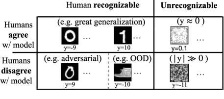
Given the recent trend of applying NNs to open-world, non-IID applications (Cao et al., 2022; Sun & Li, 2022), we argue that it is crucial to obtain the complete output distribution of a trained NN over the entire input space. This output distribution can offer a complete picture about the number of inputs mapped to certain output values. Note that the entire input space here includes all kinds of inputs mentioned above and even human unrecognizable inputs (see Figure 2(a)). As a pilot study, we focus on binary classification — given a trained binary NN classifier, we aim to sample the entire input space to obtain the output distribution, i.e., a histogram that counts the number of input samples mapped to certain logit values, as shown in Fig 2(b). The sampling procedure would also offer more fine-grained information as side products, such as representative input samples corresponding to a certain range of output values.
A straightforward solution is exhaustive enumeration or traditional Monte Carlo methods (Chen et al., 2014; Welling & Teh, 2011; Li et al., 2016; Xu et al., 2018). However, the sampling time would become impractical, or the sampler could get stuck in a subset of input space, especially for high-dimensional inputs. To overcome these issues, in this paper, we propose a novel sampler called Gradient-based Wang–Landau (GWL) sampling as follows.
We first connect the output distribution of a NN to the density of states (DOS) of a physical system through an analogy between the system energy and neural network output, as shown in Figure 1. From the physics point of view, the input to the neural network can be viewed as the configuration of the system; the neural network output (e.g., logit values in binary classifier) corresponds to the energy function ; the output distribution of a NN is then analogous to the DOS of a physical system, which is the number of configurations corresponding to the same energy value. The log scale of the DOS is the microcanonical entropy associated with the energy, .
Our new sampler GWL is a novel renovation of the classic sampler for the DOS problem, Wang–Landau algorithm (Wang & Landau, 2001), where we replace its random proposals with gradient-based Monte Carlo proposals. Given the overwhelming number of human unrecognizable inputs in the entire input space, if one adopts the traditional Monte Carlo proposal in the Wang–Landau algorithm, i.e., by changing pixel values at random, the sampling process is likely to get stuck in this human unrecognizable subset. Thus, we propose to apply a gradient-based proposal following Gibbs-with-Gradients (Grathwohl et al., 2021), which proves to be efficient to propose in-distribution inputs for a trained NN model. This way, our GWL sampler investigates the under-sampled subsets of the input space much more efficiently. The accuracy of GWL has been empirically verified on a small toy dataset — the output distribution generated by GWL aligns perfectly with the result of exhaustive enumeration.
More importantly, by analyzing the output distribution generated by GWL, we showcase several interesting findings of CNN and ResNet in a binary classification task based on real-world pictures. First, our experiments show that in both CNN and ResNet, the dominant output values are very negative and the vast majority of them correspond to human-unrecognizable input images. This supplies direct evidence to the well-known overconfidence issue in NNs (Nguyen et al., 2015). Second, when we focus on the output values where the in-distribution inputs correspond to, human-unrecognizable inputs still dominate significantly. This result presents significant challenges to the out-of-distribution (OOD) detection problems. Third, we observe a clear background darkness pattern of the representative samples of CNN and ResNet when the output logit value increases, and speculate these models simply utilize such “backdoors” to predict the labels of the digits without truly understanding the semantics of the images.
In summary, we demonstrate that sampling the entire input space to obtain the output distribution of a trained NN is computationally feasible, and it can provide new and interesting insights for future systematic investigation. Our contributions are summarized as follows.
-
•
We tackle the challenging yet important problem to uncover the output distribution of a NN over the entire input space. Such output distribution offers a novel perspective to understand NNs.
-
•
We connect this output distribution to the DOS in physics and successfully renovate the Wang–Landau algorithm using a gradient-based proposal, which is a critical component to sample the entire output space as much as possible, and to improve efficiency.
-
•
We conduct extensive experiments on toy and real-world datasets to confirm the accuracy of our proposed sampler.
-
•
GWL sampler allows for detailed investigation of the input-output mapping of NNs, facilitating further studies systematically.
2 Problem definition
In the traditional setting, binary neural classifiers model the class distribution through logit . A neural classifier parameterized by learns through a function , where , for images, and is the Dirac delta function. aligns with Gibbs-With-Gradient’s setting to be discrete.
The above model does not define the distribution of the data . This work aims to obtain the output value distribution of binary classifiers in the entire input space: . Here we assume that the input follows a uniform distribution over the domain of . We define the joint distribution
Our goal is to obtain the logit (output) distribution , which can be obtained by marginalizing the joint distribution over the input space :
To sample from the distribution , we can first sample , then condition on the sampled to obtain . While a uniform sampler in principle can solve this problem, it can take an impractically long time to converge.
3 Method
In this section, we discuss the connection between our problem to the density of states (DOS), introduce both Wang-Landau algorithm and the Gibbs-With-Gradient proposal method as a background, and present our new sampler Gradient-Wang-Landau (GWL) algorithm.
3.1 Connection to Density of States in Physics
In statistical physics, given the energy function , the DOS is defined as
where is the Dirac delta function and is the domain of where is valid. The DOS can be viewed as a probability distribution in the energy space; its log-probability defines the entropy :
Boltzmann constant is taken to be in our setting. DOS is meaningful because many physical quantities depend on energy or its integration but not the specific input .
We associate the neural network output distribution to DOS in physics by making an analogy between the system energy and NN output . This connection is based on the observation that the energy function in physics maps an input configuration to a scalar-valued energy; similarly, a binary neural classifier maps an image to a logit. Both the logit and energy are treated as the direct output of the mapping. Other quantities, such as the loss, are derived from the output. The desired output distribution can be obtained similarly as sampling the DOS in physics, which is the count of the configurations given an energy value. The output distribution and DOS are both defined in the entire input space.
3.2 Traditional Samplers Are Not Directly Applicable
Traditional Monte Carlo (MC) samplers (Chen et al., 2014; Welling & Teh, 2011; Li et al., 2016; Xu et al., 2018), in principle, could be applied to sample the output distribution, but they would not be efficient to our study. This is because these algorithms bias the sampler to the more probable domain based on importance sampling. Consequently, a major drawback is that the sampler is easily “stuck” in some localized distributions as it is hard for the sampler to overcome the barriers to visit all the possible configurations (or input images in the NN case). This limitation is particularly severe when sampling from multi-modal distributions. Our problem setting, however, not only requires the sampler to sample from a multi-modal distribution. More importantly, the target distribution is unknown upfront and the generated samples have to cover the whole output space. Using traditional MC samplers, in the best case scenario, would take an unreasonable time to converge. In the more critical but likely scenario, there is a high risk of obtaining samples that do not truly represent the underlying distribution.
3.3 Wang-Landau algorithm and Gibbs-With-Gradient
Wang–Landau (WL) algorithm was originally designed to determine the DOS of a physical system (Wang & Landau, 2001), when the DOS is not known a priori and would be determined on-the-fly. It is therefore a suitable tool for estimating the true distribution of our NN output as it is also unknown before the sampling. WL uses a histogram to store the instantaneous estimation . WL improves the sampling efficiency by using the inverted distribution as the sampling weight :
The instantaneous entropy is updated iteratively until convergence. At the end of the simulation, when the estimation of the entropy approaches the true value , the sampler would sample the entire output space uniformly.
Previous work on the sampling of a complex physics system has shown that with the same number of MC steps, WL was able to successfully produce the correct distribution when the traditional Metropolis MC sampling fail (Li et al., 2012). This is because WL can overcome energy barriers by accumulating the counts of visits and uses their inverse as sampling biases, a mechanism that traditional MC samplers are missing.
The Gibbs-With-Gradients (GWG) method is used for energy-based models (EBM) by sampling
where is the unnormalized log-probability, is the partition function, and is discrete. Typical Gibbs sampler iterates every dimension of , computes the conditional probability , and samples according to this conditional probability.
When the training data are natural images and the EBM learns decently well, the traditional Gibbs sampler wastes much of the computation. For example, most pixel-by-pixel iterations over in MNIST dataset will be on the black background. GWG proposes a smart proposal that picks the pixel that is more likely to change, such as the pixels around the edge between the bright and dark region of the digits.
3.4 Wang–Landau with Gradient Proposal
Directly applying WL algorithm with random proposals is insufficient to sample the output space efficiently, because a trained neural model learns a preferred mapping through the loss function. For example, a binary classifier maps the training inputs to either the sufficiently positive or negative logit values, which ideally should correspond to the extremely rare but semantically meaningful inputs. After the sampler explores and generates the peak centered at 0 where most random samples correspond to (Fig. 2(b)), it is almost impossible for the sampler with a random proposal to propose an input with meaningful structure (or even in-distribution inputs) so that the other possible output values are explored. Of course, whether those output values correspond to in-distribution inputs is only confirmable after sampling. In summary, it is extremely difficult for the random proposal in WL algorithm to explore all the possible output values.
We therefore propose to use the Wang–Landau algorithm framework but replace the MC proposal with the one in Gibbs-With-Gradients (GWG) sampler. GWG has a gradient proposal that takes advantage of the model’s learned weights to propose inputs. In order to sample the distribution of the output prediction through GWG, we define log-probability as:
where is the count in log scale for the bin corresponding to . The fixed in the original GWG is now changing in our sampling process given the input , since the expression for is unknown and we can only estimate the output distribution from using WL algorithm. GWG requires the gradient of , but since is approximated using discrete bins, we apply a first-order differentiable interpolation for taking the derivative of the discrete histogram of entropy.
Similar to the original WL algorithm, we first initialize two histograms with all of their bins set to 0. One of these histograms is for estimating entropy , and the other histogram, , is a counter of how many times the sampler has visited a specific bin. is also used for checking if all the bins have been visited roughly equally, i.e., a flatness check. We first preset the number of iterations that the sampling will perform, as well as a modification factor that is used to update the estimation of entropy iteratively. At each MC step,we interpolate to get a differentiable interpolation, take the derivative of the negation of with respect to the output and then the inputs using chain rule. GWG uses this gradient to propose the next input that is likely to have a lower entropy and be accepted by the sampler. The newly proposed input sample is then accepted or rejected according the acceptance probability:
where q is the proposal distribution. When a proposal is accepted, the entropy of the corresponding output value is updated using the modification factor . Otherwise the of the “old” output value will be updated. This sampling procedure repeats until the histogram passes the flatness check. The sampler then enters the next iteration with the counters in reset to 0, reduced by half, but the histogram kept for further accumulation. This sampling procedure drives the sampler to visit rare samples whose logit values correspond to the lower entropy, while providing an estimation of entropy as a result at the end. This proposed algorithm is provided in Alg. 1 in Appendix.
4 Related Works and Discussions
Performance Characterization has long been explored even before the era of deep learning (Haralick, 1992; Klette et al., 2000; Thacker et al., 2008). The input-output relationship has been explored for simple functions (Hammitt & Bartlett, 1995) and mathematical morphological operators (Gao et al., 2002; Kanungo & Haralick, 1990). Compared to existing performance characterization approaches (Ramesh et al., 1997; Bowyer & Phillips, 1998; Aghdasi, 1994; Ramesh & Haralick, 1992, 1994), our work focuses on the output distribution (Greiffenhagen et al., 2001) of a neural network over the entire input space (i.e., not task specific) following the blackbox approach (Courtney et al., 1997; Cho et al., 1997) where the system transfer function from input to output is unknown. Our setting shall be viewed as the most general forward uncertainty quantification case (Lee & Chen, 2009) where the model performance is characterized when the inputs are perturbed (Roberts et al., 2021). To our best knowledge, we demonstrate for the first time that the challenging task of sampling the entire input space for modern neural networks is feasible and efficient by drawing the connection between neural network and physics models. Our proposed method can offer samples to be further integrated with the performance characterization methods mentioned above.
Density Estimation and Energy Landscape Mapping
Previous works in density estimation focus on data density (Tabak & Turner, 2013; Liu et al., 2021), where class samples are given and the goal is to estimate the density of samples. Here we are not interested in the density of the given dataset, but the density of all the valid samples in the pixel space for a trained model. (Hill et al., 2019; Barbu & Zhu, 2020) have done the pioneering work in sampling the energy landscape for energy-based models. Their methods specifically focus on the local minimum and barriers of the energy landscape. We can relax the requirement and generalize the mapping on the “output” space where either sufficiently positive or sufficiently negative output (logit) values are meaningful in binary classifiers and other models.
Open-world Model Evaluation
Though many neural models have achieved the SOTA performance, most of them are only on in-distribution test sets (Dosovitskiy et al., 2021; Tolstikhin et al., 2021; Steiner et al., 2021; Chen et al., 2021; Zhuang et al., 2022; He et al., 2015; Simonyan & Zisserman, 2014; Szegedy et al., 2015; Huang et al., 2017; Zagoruyko & Komodakis, 2016). Open-world settings where the test set distribution differs from the in-distribution training set create special challenges for the model. While the models have to detect the OOD samples from in-distribution samples (Liu et al., 2020; Hendrycks & Gimpel, 2016; Hendrycks et al., 2019; Hsu et al., 2020; Lee et al., 2017, 2018; Liang et al., 2018; Mohseni et al., 2020; Ren et al., 2019), we also expect sometimes the model could generalize what it learns to OOD datasets (Cao et al., 2022; Sun & Li, 2022). It has been discovered that models have over-confident predictions for some OOD samples that obviously do not align with human judgments (Nguyen et al., 2015). The OOD generalization becomes more challenging because of this discovery, because the models may not be as reliable as we thought they were. Adversarial test sets (Szegedy et al., 2013; Rozsa et al., 2016; Miyato et al., 2018; Kurakin et al., 2016; Xie et al., 2019; Madry et al., 2017) also present special challenges as models decisions are different from those of humans. Having a full view of input-output relation with all the above different kinds of test sets under consideration is important.
Samplers
MCMC samplers (Chen et al., 2014; Welling & Teh, 2011; Li et al., 2016; Xu et al., 2018) are developed to scale to big datasets and sample efficient with gradients. Recently, Gibbs-With-Gradients (GWG) (Grathwohl et al., 2021) is proposed to pick the promising pixel(s) as the proposal. To further improve sampling efficiency, CSGLD (Deng et al., 2020) drives the sampler to explore the under-explored energy using similar idea as Wang–Landau algorithm (Wang & Landau, 2001). The important difference between our problem setting and the previous ones solved by other MCMC samplers is the function or model as distribution to be sampled from is unknown. Wang–Landau algorithm utilizes previous approximation of the distribution to drive the sampler to explore the under-explored energy regions. This algorithm can be more efficient through parallelization (Vogel et al., 2013; Cunha-Netto et al., 2008), assumption about continuity in output space (Junghans et al., 2014; Li & Eisenbach, 2017) and extension to multi-dimensional outputs (Zhou et al., 2006). While the previous samplers can be applied to high-dimensional inputs, the energy functions in physics are relative simple and symmetric. However, modern neural networks are complex and hard to characterize performance (Roberts et al., 2021). We assume agnostic of the output properties of the model and thus apply the Wang–Landau algorithm to sample the entropy as a function of energy but with the gradient proposal in GWG to make the sampler more efficient. Similar to GWG, our sampler can propose the inputs corresponding to the under-explored regions of outputs. Improvements of efficiency can benefit from a patch of pixel changes.
5 Experiments
In this section, we apply our proposed Gradient Wang–Landau sampler to inspect a few neural network models and present the discovered output histogram together with representative samples. The dataset and model training details are introduced in Sec. 5.1. We first empirically confirm our sampler performance through a toy example in Sec. 5.2. We then discuss results for modern binary classifiers in Sec. 5.3 and Sec. 5.4. Hyperparameters of the samplers tested in are Appendix C.
5.1 Datasets, Models, and Other Experiment Settings
Datasets
As aforementioned, we focus on binary classification. Therefore, we derive two datasets from the MNIST datasets by only including samples with labels . The training and test splits are the same as those in the original MNIST dataset.
-
•
Toy is a simple dataset with binary input images we construct. It is designed to make feasible the bruteforce enumeration over the entire input space (only different samples). We center crop the MNIST samples from classes and resize them to images. We compute the average of the pixel values and use the average as the threshold to binarize the images — the pixel value lower than this threshold becomes ; otherwise, it becomes . The duplicates are not removed for accuracy after resizing since PyTorch does not find duplicate row indices.
-
•
MNIST-0/1 is an MNIST dataset whose samples only have the 0,1 labels. To align with the GWG setting, the inputs are discrete and not Z-normalized. Therefore, in this dataset, the input is dimensional with discrete pixel values from .
Neural Network Models for Evaluation
Since the focus of this paper is not to compare different neural architectures, given the relatively small datasets we have, we train two types of models, a simple CNN and ResNet-18 (He et al., 2015). Each pixel of the inputs is first transformed to the one-hot encoding and passed to a 3-by-3 convolution layer with 3 channel output. The CNN model contains 2 convolution layers with 3-by-3 filter size. The output channels are 32 and 128. The final features are average-pooled and passed to a fully-connected layer for the binary classification.
Please keep in mind that our goal in this experiment section is to showcase that our proposed sampler can uncover some novel interesting empirical insights for neural network models. Models with different architectures, weights due to different initialization, optimization, and/or datasets will lead to different results. Therefore, our results and discussions are all model-specific. Specifically, we train a simple CNN model to classify the binary images in the Toy dataset (CNN-Toy). The test accuracy of this CNN-Toy model reaches , which is almost perfect. We train a simple CNN model to classify the grey-scale images in the MNIST-0/1 dataset (CNN-MNIST-0/1). The test accuracy of CNN-MNIST-0/1 model is . We train a ResNet-18 model to classify the grey-scale images in the MNIST-0/1 dataset (ResNet-18-MNIST-0/1). The test accuracy of ResNet-18-MNIST-0/1 model is .
Sampling Methods for Comparison
We compare several different sampling methods (including our proposed method) to obtain the output histogram over the entire input space.
-
•
Enumeration generates the histogram by enumerating all the possible pixel values as inputs. This is a rather slow but the most accurate method.
-
•
In-dist Test Samples generates the histogram of the inputs based on the fixed test set.This is commonly used in machine learning evaluation. It is based on a very small and potentially biased subset of the entire input space.
-
•
Wang-Landau algorithm (WL) generates the histogram the Wang-Landau algorithm with the random proposal. Specifically, we randomly pick one pixel at a time and change it to any valid (discrete) value as in this implementation 111https://www.physics.rutgers.edu/~haule/681/src_MC/python_codes/wangLand.py.
-
•
Gradient Wang-Landau (GWL) generates the histogram by our proposed sampler of Wang-Landau algorithm with gradient proposal.

5.2 Results of CNN-Toy
Given the CNN-Toy model, we apply Enumeration, GWL, and In-dist Test Samples to obtain the output entropy histograms, as shown in Fig. 3. Note that our GWL method samples the relative entropy of different energy values as duplicate may be proposed. After normalization with the maximum entropy, the GWL histogram almost exactly matches the Enumeration histogram which is the ground truth histogram. This confirms the accuracy of our GWL sampler and we can apply it further to more complicated models with confidence.
Remarkably, this histogram is quite different from the expectation we presented in Fig. 2(b) — this histogram is even not centered at or has the expected subdominant peaks on both the positive and negative sides. Instead, the dominant peak is so wide that it covers almost the entire spectrum of the possible output values. From a coarse-grained overview, most of the samples are mapped to the center of logit with a decay from to both sides in the CNN-Toy model. This shows the CNN-Toy model is biased to predict more samples to the negative logit values.
In Fig. 3, we also present the representative samples obtained by GWL given different logit values in the CNN-Toy model. Our conjectured analysis of the representative samples are in Appendix B. From this example, one can see that the output histogram over the entire input space can offer a comprehensive understanding of the neural network models, helping researchers better understand critical questions such as the distribution of the outputs, where the model maps the samples to, and what the representative samples with high likelihood are.

5.3 Results of CNN-MNIST-0/1
Entropy Histogram from GWL
The application of GWL on the CNN-Toy model is encouraging. Now we apply GWL to the CNN-MNIST-0/1 that is trained on a real-world dataset. The results from the iteration are shown in Fig. 4. As our GWL reveals, the output histogram of CNN-MNIST-0/1, similar to CNN-Toy’s histogram, does not have the subdominant peaks. It is also different from the presumed case in Fig. 2(b). Compared with the output histogram of the CNN-Toy model (i.e., Fig. 3), for the CNN-MNIST-0/1 case, the peak is on the negative boundary and the histogram is skewed towards the negative logit values. monotonically decreases as the logit values go from negative to positive. While the in-distribution samples have logit values between and as we expect, these samples are exponentially (i.e., at logit value -20 to at logit value 18, thousands in log scale) less often found than the majority samples whose logit values are around . From a fine-grained view, the CNN-MNIST-0/1 model tends to map the human-unrecognizable samples to the very negative logit values. While previous work (Nguyen et al., 2015) showed the existence of the overconfident prediction samples, our result shows a rough but quantitative performance of this CNN which can serve as a baseline for further improvements.
GWL is much more efficient than WL
We first confirm the correctness of our WL sampler on a Ising model and apply it to this CNN model. WL takes a much longer time to converge and we are not able to obtain the converged results. Both WL and GWL cannot have more than 1 worker writing to the same set of DOS bins or else incorrect DOS will be resulted (Yin & Landau, 2012). For comparison, we inspect the intermediate results of the GWL and WL samplers, as shown in Fig. 5. As one can see from Fig. 5(a), GWL is already able to explore the logit values efficiently from the most dominant output value around to the positive logit values in the first iteration. Within only two iterations (Fig. 5(b)), GWL can discover the output histogram covering the value range from to . On the other hand, as presented in Fig. 5(c), the original WL can only explore the output ranges from around to for 60,000,000 steps (around 10 days without much substantial progress). WL converges significantly slower and never ends in a reasonable time. This result indicates that the GWL converges much faster than the original WL and is able to explore a much wider range of output values.


Manual inspection on more representative samples
As show in Fig. 4, for the CNN-MNIST-0/1 model, GWL can effectively sample input images from logit values ranging from -55 to 18. We further group these logit values per 5 unit of logit value in . For every group, we sample 200 representative input images. To make sure they are not correlated, we sample every 50000 pixel changes. For demonstration purposes, we randomly pick 10-out-of-200 samples from every group in Fig. 7(a) in Appendix. We manually inspect the sufficiently positive group (e.g., the last column in Fig. 7(a)) and the sufficiently negative groups (e.g., the first five columns in Fig. 7(a)) , and there are no human recognizable samples of digits. We also observe an interesting pattern that as the logit value increases, more and more representative samples have black background. This result suggests that the CNN-MNIST-0/1 model may heavily rely on the background to classify the images (Xiao et al., 2020). We conjecture that is because the samples in the most dominant peak are closer to class 0 samples than class 1 samples and this is supported by experimental results (see Appendix. D). More rigorous experiments to a definite conclusion is yet required as future work. In summary, although CNN-MNIST-0/1 holds a very high in-distribution test accuracy, it is far from a robust model because it does not truly understand the semantic structure of the digits.
Discussion
Fig. 4 presents challenges to the OOD detection methods that may be more model-dependent than we thought before. If the model cannot map most of the human unrecognizable samples with high uncertainty, the likelihood-based OOD detection methods (Liu et al., 2020; Hendrycks & Gimpel, 2016) cannot perform well for samples in the entire input space. Fig. 7(a) shows the inputs with the in-distribution output values (output logits of the red plot) of the CNN model may not uniquely correspond to in-distribution samples. More rigorous experiments to a definite conclusion are yet required as future work.
5.4 Results of ResNet-18-MNIST-0/1
Entropy Histogram from GWL
When applying our GWL samplers to the ResNet-18-MNIST-0/1 model, for iteration (Fig. 6(a)), we observe that the sampler discovers a wide range of negative logit values from around logit value of -220 to around -33, much wider than that of the CNN’s. This range of negative logits, however, does not correspond to human recognizable inputs and there is no obvious pattern observed in contrast to CNN-MNIST-0/1’s results. It means the ResNet-18-MNIST-0/1 model makes more confident predictions for some samples than the CNN-MNIST-0/1 model does. Moreover, we observe a cliff around the logit value of -33 and thus we specifically sample the region from -30 to 20 and generate the representative samples in this region where the in-distribution logits fall into. Fig. 6(b) shows the entropy histogram after the iteration. Some output regions of the in-distribution samples take longer time to discover. This calls for a more efficient sampler in the future.
Manual inspection on more representative samples
Interestingly, similar (if not exactly the same) pixel patterns for CNN-MNIST-0/1 model appear, as shown in Fig. 6(b) and Fig. 7(b). The representative samples, however, have broader noisy boundaries compared to those from the CNN-MNIST-0/1 model. The same phenomenon also happens that the double peaks of the test set samples do not align with the output distribution of the entire input space.
Because of the complexity of ResNet-18 over CNN and it takes a longer time to converge, we do not draw conclusions about ResNet-18-MNIST-0/1 evaluation of the entropy difference. Compared with the CNN-MNIST-0/1 model, ResNet-18-MNIST-0/1 has more interesting phenomena for further exploration.
6 Conclusion
We aim to get a full picture of the input-output relationship of a model through the inputs valid in the pixel space. We propose to obtain a histogram to estimate the entropy in the output space to better understand the input-output distribution. When the inputs are high-dimensional, enumeration or uniform sampling is either impossible or takes too long to converge. We connect the density of states in physics to this histogram of output entropy. We propose a new, efficient sampler, Wang–Landau sampling with gradient proposals, to achieve this goal. We confirm empirically this can be achieved and uncover some new aspects of neural networks.
We observe several limitations. First, though we combine two samplers that have the theoretical guarantee of convergence and confirm the performance of the sampler through empirical results, we do not provide a proof of convergence when they are combined. Second, because of the nature of our problem, we observe that the sampler still takes a decent amount of time to converge, especially for the more complicated network architectures such as ResNet. We avoid making conclusions on the distributions but provide some observations for ResNet. The sampler for ResNet is still converging but it also calls for further development of faster samplers for these more complicated networks. Third, even though the ratio of the recognizable samples can be derived from our sampler, our CNN model maps an enormous amount of samples to the desired output region of the in-distribution inputs, and we do not observe even one human recognizable sample out of the hundreds of representative samples. Future automatic methods can alleviate the need of human labels.
For future work, it is necessary to develop new and more efficient samplers that have theoretical guarantees to acquire this input-output relationship in order to sample with more pixels, such as the ImageNet (Deng et al., 2009). Most importantly, we can then develop new insights into network architectures developed in the last decade for open-world applications using these efficient samplers.
References
- Aghdasi (1994) Aghdasi, F. Digitization and analysis of mammographic images for early detection of breast cancer. PhD thesis, University of British Columbia, 1994.
- Barbu & Zhu (2020) Barbu, A. and Zhu, S.-C. Mapping the energy landscape. In Monte Carlo Methods, pp. 367–420. Springer, 2020.
- Bowyer & Phillips (1998) Bowyer, K. and Phillips, P. J. Empirical evaluation techniques in computer vision. IEEE Computer Society Press, 1998.
- Cao et al. (2022) Cao, K., Brbic, M., and Leskovec, J. Open-world semi-supervised learning. In International Conference on Learning Representations, 2022. URL https://openreview.net/forum?id=O-r8LOR-CCA.
- Chen et al. (2014) Chen, T., Fox, E., and Guestrin, C. Stochastic gradient hamiltonian monte carlo. In International conference on machine learning, pp. 1683–1691. PMLR, 2014.
- Chen et al. (2021) Chen, X., Hsieh, C.-J., and Gong, B. When vision transformers outperform resnets without pretraining or strong data augmentations. arXiv preprint arXiv:2106.01548, 2021.
- Cho et al. (1997) Cho, K., Meer, P., and Cabrera, J. Performance assessment through bootstrap. IEEE Transactions on Pattern Analysis and Machine Intelligence, 19(11):1185–1198, 1997.
- Courtney et al. (1997) Courtney, P., Thacker, N., and Clark, A. F. Algorithmic modelling for performance evaluation. Machine Vision and Applications, 9(5):219–228, 1997.
- Cunha-Netto et al. (2008) Cunha-Netto, A. G. d., Caparica, A., Tsai, S.-H., Dickman, R., and Landau, D. P. Improving wang-landau sampling with adaptive windows. Physical Review E, 78(5):055701, 2008.
- Deng et al. (2009) Deng, J., Dong, W., Socher, R., Li, L.-J., Li, K., and Fei-Fei, L. Imagenet: A large-scale hierarchical image database. In 2009 IEEE Conference on Computer Vision and Pattern Recognition, pp. 248–255, 2009. doi: 10.1109/CVPR.2009.5206848.
- Deng et al. (2020) Deng, W., Lin, G., and Liang, F. A contour stochastic gradient langevin dynamics algorithm for simulations of multi-modal distributions. In Advances in Neural Information Processing Systems, 2020.
- Dosovitskiy et al. (2021) Dosovitskiy, A., Beyer, L., Kolesnikov, A., Weissenborn, D., Zhai, X., Unterthiner, T., Dehghani, M., Minderer, M., Heigold, G., Gelly, S., Uszkoreit, J., and Houlsby, N. An image is worth 16x16 words: Transformers for image recognition at scale. ICLR, 2021.
- Gao et al. (2002) Gao, X., Ramesh, V., and Boult, T. Statistical characterization of morphological operator sequences. In European Conference on Computer Vision, pp. 590–605. Springer, 2002.
- Grathwohl et al. (2021) Grathwohl, W., Swersky, K., Hashemi, M., Duvenaud, D., and Maddison, C. Oops i took a gradient: Scalable sampling for discrete distributions. In International Conference on Machine Learning, pp. 3831–3841. PMLR, 2021.
- Greiffenhagen et al. (2001) Greiffenhagen, M., Comaniciu, D., Niemann, H., and Ramesh, V. Design, analysis, and engineering of video monitoring systems: An approach and a case study. Proceedings of the IEEE, 89(10):1498–1517, 2001.
- Hammitt & Bartlett (1995) Hammitt, A. and Bartlett, E. Determining functional relationships from trained neural networks. Mathematical and computer modelling, 22(3):83–103, 1995.
- Haralick (1992) Haralick, R. M. Performance characterization in computer vision. In BMVC92, pp. 1–8. Springer, 1992.
- He et al. (2015) He, K., Zhang, X., Ren, S., and Sun, J. Deep residual learning for image recognition. arXiv preprint arXiv:1512.03385, 2015.
- Hendrycks & Gimpel (2016) Hendrycks, D. and Gimpel, K. A baseline for detecting misclassified and out-of-distribution examples in neural networks. arXiv preprint arXiv:1610.02136, 2016.
- Hendrycks et al. (2019) Hendrycks, D., Mazeika, M., and Dietterich, T. Deep anomaly detection with outlier exposure. In International Conference on Learning Representations, 2019. URL https://openreview.net/forum?id=HyxCxhRcY7.
- Hill et al. (2019) Hill, M., Nijkamp, E., and Zhu, S.-C. Building a telescope to look into high-dimensional image spaces. Quarterly of Applied Mathematics, 77(2):269–321, 2019.
- Hsu et al. (2020) Hsu, Y.-C., Shen, Y., Jin, H., and Kira, Z. Generalized ODIN: Detecting out-of-distribution image without learning from out-of-distribution data. In Proceedings of the IEEE/CVF Conference on Computer Vision and Pattern Recognition, pp. 10951–10960, 2020.
- Huang et al. (2017) Huang, G., Liu, Z., Van Der Maaten, L., and Weinberger, K. Q. Densely connected convolutional networks. In Proceedings of the IEEE conference on computer vision and pattern recognition, pp. 4700–4708, 2017.
- Junghans et al. (2014) Junghans, C., Perez, D., and Vogel, T. Molecular dynamics in the multicanonical ensemble: Equivalence of wang–landau sampling, statistical temperature molecular dynamics, and metadynamics. Journal of chemical theory and computation, 10(5):1843–1847, 2014.
- Kanungo & Haralick (1990) Kanungo, T. and Haralick, R. M. Character recognition using mathematical morphology. In Proc. of the Fourth USPS Conference on Advanced Technology, pp. 973–986, 1990.
- Klette et al. (2000) Klette, R., Stiehl, H. S., Viergever, M. A., and Vincken, K. L. Performance characterization in computer vision. Springer, 2000.
- Kurakin et al. (2016) Kurakin, A., Goodfellow, I., Bengio, S., et al. Adversarial examples in the physical world, 2016.
- Lee et al. (2017) Lee, K., Lee, H., Lee, K., and Shin, J. Training confidence-calibrated classifiers for detecting out-of-distribution samples. arXiv preprint arXiv:1711.09325, 2017.
- Lee et al. (2018) Lee, K., Lee, K., Lee, H., and Shin, J. A simple unified framework for detecting out-of-distribution samples and adversarial attacks. In Advances in Neural Information Processing Systems, pp. 7167–7177, 2018.
- Lee & Chen (2009) Lee, S. H. and Chen, W. A comparative study of uncertainty propagation methods for black-box-type problems. Structural and multidisciplinary optimization, 37(3):239–253, 2009.
- Li et al. (2016) Li, C., Chen, C., Carlson, D., and Carin, L. Preconditioned stochastic gradient langevin dynamics for deep neural networks. In Thirtieth AAAI Conference on Artificial Intelligence, 2016.
- Li & Eisenbach (2017) Li, Y. W. and Eisenbach, M. A histogram-free multicanonical monte carlo algorithm for the basis expansion of density of states. In Proceedings of the Platform for Advanced Scientific Computing Conference, pp. 1–7, 2017.
- Li et al. (2012) Li, Y. W., Wüst, T., and Landau, D. P. Surface adsorption of lattice hp proteins: Thermodynamics and structural transitions using wang-landau sampling. In Journal of Physics: Conference Series, volume 402, pp. 012046. IOP Publishing, 2012.
- Liang et al. (2018) Liang, S., Li, Y., and Srikant, R. Enhancing the reliability of out-of-distribution image detection in neural networks. In 6th International Conference on Learning Representations, ICLR 2018, 2018.
- Liu et al. (2021) Liu, Q., Xu, J., Jiang, R., and Wong, W. H. Density estimation using deep generative neural networks. Proceedings of the National Academy of Sciences, 118(15):e2101344118, 2021.
- Liu et al. (2020) Liu, W., Wang, X., Owens, J., and Li, Y. Energy-based out-of-distribution detection. Advances in Neural Information Processing Systems, 2020.
- Madry et al. (2017) Madry, A., Makelov, A., Schmidt, L., Tsipras, D., and Vladu, A. Towards deep learning models resistant to adversarial attacks. arXiv preprint arXiv:1706.06083, 2017.
- Miyato et al. (2018) Miyato, T., Maeda, S.-i., Koyama, M., and Ishii, S. Virtual adversarial training: a regularization method for supervised and semi-supervised learning. IEEE transactions on pattern analysis and machine intelligence, 41(8):1979–1993, 2018.
- Mohseni et al. (2020) Mohseni, S., Pitale, M., Yadawa, J., and Wang, Z. Self-supervised learning for generalizable out-of-distribution detection. Proceedings of the AAAI Conference on Artificial Intelligence, 34(04):5216–5223, April 2020. ISSN 2159-5399. doi: 10.1609/aaai.v34i04.5966.
- Nguyen et al. (2015) Nguyen, A., Yosinski, J., and Clune, J. Deep neural networks are easily fooled: High confidence predictions for unrecognizable images. In Proceedings of the IEEE Conference on Computer Vision and Pattern Recognition, pp. 427–436, 2015.
- Ramesh & Haralick (1994) Ramesh, V. and Haralick, R. A methodology for automatic selection of iu algorithm tuning parameters. In ARPA Image Understanding Workshop, 1994.
- Ramesh & Haralick (1992) Ramesh, V. and Haralick, R. M. Random perturbation models and performance characterization in computer vision. In Proceedings 1992 IEEE Computer Society Conference on Computer Vision and Pattern Recognition, pp. 521–522. IEEE Computer Society, 1992.
- Ramesh et al. (1997) Ramesh, V., Haralick, R., Bedekar, A., Liu, X., Nadadur, D., Thornton, K., and Zhang, X. Computer vision performance characterization. RADIUS: Image Understanding for Imagery Intelligence, pp. 241–282, 1997.
- Ren et al. (2019) Ren, J., Liu, P. J., Fertig, E., Snoek, J., Poplin, R., Depristo, M., Dillon, J., and Lakshminarayanan, B. Likelihood ratios for out-of-distribution detection. In Advances in Neural Information Processing Systems, pp. 14680–14691, 2019.
- Roberts et al. (2021) Roberts, D. A., Yaida, S., and Hanin, B. The principles of deep learning theory. arXiv preprint arXiv:2106.10165, 2021.
- Rozsa et al. (2016) Rozsa, A., Rudd, E. M., and Boult, T. E. Adversarial diversity and hard positive generation. In Proceedings of the IEEE Conference on Computer Vision and Pattern Recognition Workshops, pp. 25–32, 2016.
- Simonyan & Zisserman (2014) Simonyan, K. and Zisserman, A. Very deep convolutional networks for large-scale image recognition. arXiv preprint arXiv:1409.1556, 2014.
- Steiner et al. (2021) Steiner, A., Kolesnikov, A., , Zhai, X., Wightman, R., Uszkoreit, J., and Beyer, L. How to train your vit? data, augmentation, and regularization in vision transformers. arXiv preprint arXiv:2106.10270, 2021.
- Sun & Li (2022) Sun, Y. and Li, Y. Open-world contrastive learning. arXiv preprint arXiv:2208.02764, 2022.
- Szegedy et al. (2013) Szegedy, C., Zaremba, W., Sutskever, I., Bruna, J., Erhan, D., Goodfellow, I., and Fergus, R. Intriguing properties of neural networks. arXiv preprint arXiv:1312.6199, 2013.
- Szegedy et al. (2015) Szegedy, C., Liu, W., Jia, Y., Sermanet, P., Reed, S., Anguelov, D., Erhan, D., Vanhoucke, V., and Rabinovich, A. Going deeper with convolutions. In Proceedings of the IEEE conference on computer vision and pattern recognition, pp. 1–9, 2015.
- Tabak & Turner (2013) Tabak, E. G. and Turner, C. V. A family of nonparametric density estimation algorithms. Communications on Pure and Applied Mathematics, 66(2):145–164, 2013.
- Thacker et al. (2008) Thacker, N. A., Clark, A. F., Barron, J. L., Beveridge, J. R., Courtney, P., Crum, W. R., Ramesh, V., and Clark, C. Performance characterization in computer vision: A guide to best practices. Computer vision and image understanding, 109(3):305–334, 2008.
- Tolstikhin et al. (2021) Tolstikhin, I., Houlsby, N., Kolesnikov, A., Beyer, L., Zhai, X., Unterthiner, T., Yung, J., Steiner, A., Keysers, D., Uszkoreit, J., Lucic, M., and Dosovitskiy, A. Mlp-mixer: An all-mlp architecture for vision. arXiv preprint arXiv:2105.01601, 2021.
- Vogel et al. (2013) Vogel, T., Li, Y. W., Wüst, T., and Landau, D. P. Generic, hierarchical framework for massively parallel wang-landau sampling. Physical review letters, 110(21):210603, 2013.
- Wang & Landau (2001) Wang, F. and Landau, D. P. Efficient, multiple-range random walk algorithm to calculate the density of states. Physical review letters, 86(10):2050, 2001.
- Welling & Teh (2011) Welling, M. and Teh, Y. W. Bayesian learning via stochastic gradient langevin dynamics. In Proceedings of the 28th international conference on machine learning (ICML-11), pp. 681–688, 2011.
- Xiao et al. (2020) Xiao, K., Engstrom, L., Ilyas, A., and Madry, A. Noise or signal: The role of image backgrounds in object recognition. arXiv preprint arXiv:2006.09994, 2020.
- Xie et al. (2019) Xie, C., Zhang, Z., Zhou, Y., Bai, S., Wang, J., Ren, Z., and Yuille, A. L. Improving transferability of adversarial examples with input diversity. In Proceedings of the IEEE/CVF Conference on Computer Vision and Pattern Recognition, pp. 2730–2739, 2019.
- Xu et al. (2018) Xu, P., Chen, J., Zou, D., and Gu, Q. Global convergence of langevin dynamics based algorithms for nonconvex optimization. Advances in Neural Information Processing Systems, 31, 2018.
- Yin & Landau (2012) Yin, J. and Landau, D. Massively parallel wang–landau sampling on multiple gpus. Computer Physics Communications, 183(8):1568–1573, 2012.
- Zagoruyko & Komodakis (2016) Zagoruyko, S. and Komodakis, N. Wide residual networks. arXiv preprint arXiv:1605.07146, 2016.
- Zhou et al. (2006) Zhou, C., Schulthess, T. C., Torbrügge, S., and Landau, D. P. Wang-landau algorithm for continuous models and joint density of states. Phys. Rev. Lett., 96:120201, Mar 2006. doi: 10.1103/PhysRevLett.96.120201. URL https://link.aps.org/doi/10.1103/PhysRevLett.96.120201.
- Zhuang et al. (2022) Zhuang, J., Gong, B., Yuan, L., Cui, Y., Adam, H., Dvornek, N., Tatikonda, S., Duncan, J., and Liu, T. Surrogate gap minimization improves sharpness-aware training. ICLR, 2022.
Appendix A Gradient Wang-Landau Algorithm
Here we provide the algorithms of the GWL algorithm. The input and output are listed. The hyperparameters are determined mostly by the toy-example.
Appendix B Comment on Representative samples for CNN-Toy
The visualization results suggest that the CNN-Toy model probably learns the digit “1” for positive logit values as the center pixels of the representative samples are white (see the three representative samples with logit values from 0 to 20) and “0” for the very negative logit values as the center pixels of the representative samples are black (see two representative samples with logit values from -20 to -30).
Appendix C Hyper-parameters and Implementation Details for GWL and WL
The hyper-parameters for GWL and WL are extremely similar, if not identical, as the only major difference between GWL and WL is the gradient proposal versus the random proposal. We first preset a large enough range of output values for the sampler to explore the trained neural network models. In our experiments, we found that the output (logit) values of the binary classifiers typically fall in the range of -300 to 100 (based on ResNet). Therefore, we use this range for all experiments. For flatness histogram , the bin window size is set to be 1, resulting in 400 bins. The histogram is considered flat if the difference between maximum bin value and minimum bin value is smaller than the average bin value.
Appendix D Samples similarity
We conjecture that is because the samples in the most dominant peak are closer to class 0 samples than class 1 samples. We compute the L2 pixel-wise distance from the uniform noise image to the samples of class 1 and 0 respectively. The mean L2 distance from uniform noise to 0 is around 0.3121 and that from uniform noise to 1 is around 0.3236. The distance between 1 and 0 samples is 0.1652. This result shows the samples in the most dominant peak are closer to class 0 samples than class 1 samples.
Appendix E Representative inputs
Here we list more representative samples of the CNN-MNIST-0/1 scenario. The samples are bounded by a black box of boundaries.

